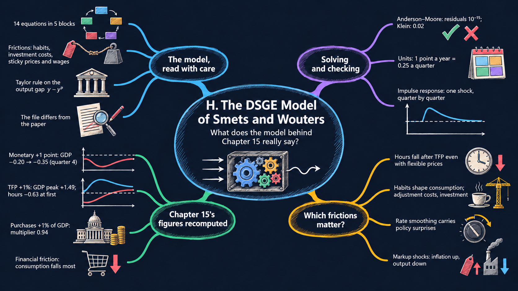
Chapter 15 ended with the impulse responses of an estimated DSGE model, the model of Frank Smets and Rafael Wouters (2007), and said that we could not recompute them. This appendix recomputes them. It is the advanced version of Chapter 15: the same storylines (TFP shocks, government purchases, sticky wages and prices, monetary policy), now in the full model that central banks use, solved in Python with the Snowdrop package of Appendix G. By the end of this appendix you will be able to:
read the 14 equations of the Smets–Wouters model, say what each one does, and link it to the simple models of Chapter 15;
read a research model file with care: find what it changes, what it gets wrong and what it leaves out;
solve the model with Snowdrop, check that the solution is right, and compute impulse responses in the units that the textbook uses;
recompute the five Smets–Wouters figures of Chapter 15 (a monetary policy shock, a TFP shock, a rise in government purchases and a financial friction shock), and compare the numbers with those that Jones (2024) reports;
run experiments: switch frictions off one at a time and find out which of them produce the patterns of Chapter 15.
The appendix assumes Chapter 15 and Appendix G (Sections G.1 to G.7). The economics of every equation is explained as it comes; the derivations from households’ and firms’ optimization problems are not, and Section H.13 says where to find them.
A map of the appendix
Section
What you do
Builds on
H.1
See what Smets and Wouters add to the model of Chapter 15
Chapter 15, Appendix G.1
H.2
Install Snowdrop and set up
Appendix G.3
H.3
Read the model, equation by equation
Chapters 12, 13, 15
H.4
Read the model file with care, and write a corrected copy
Appendix G.5
H.5
Solve the model, check the solution, define an impulse response
Appendix G.4
H.6
A monetary policy shock (textbook Figs. 15.9 and 15.10)
Chapters 12, 13
H.7
A TFP shock (textbook Fig. 15.11)
Chapters 5, 15
H.8
A rise in government purchases (textbook Fig. 15.12)
Chapters 11, 15
H.9
A financial friction shock (textbook Fig. 15.13)
Chapter 14
H.10
The three shocks that Chapter 15 does not show
—
H.11
Experiments: which frictions matter?
Chapter 15
H.12
The file’s own numbers, and the corrected equation
—
H.13
Go further
Appendix G.9–G.12
H.1 From Chapter 15 to an estimated model
Chapter 15 built a DSGE model in small pieces: TFP shocks in the Solow model, a labor market in which labor demand and labor supply set employment and the real wage, and sticky wages or sticky prices that let monetary policy move output. Each piece answered one question at a time, with “consumption taken as given”.
Smets and Wouters (2007) put all of these pieces, and more, into one model, and estimated it on U.S. data from 1966 to 2004. Their model builds on Christiano, Eichenbaum and Evans (2005). It has:
households that like consumption, with habits (they care about consumption relative to last quarter’s), and dislike work;
firms that rent capital, decide how intensively to use it (capacity utilization), and pay a cost when they change investment quickly (investment adjustment costs);
sticky prices and sticky wages: each quarter only some firms reset their prices and only some households reset their wages (the Calvo model), and the others index them to past inflation;
a central bank that sets the interest rate with a Taylor rule (Chapter 12);
seven shocks: to TFP, to a risk premium (the financial friction of textbook Fig. 15.13), to government purchases, to the efficiency of investment, to monetary policy, and to price and wage markups.
“Estimated” means that the parameters were chosen so that the model fits seven U.S. series (the growth of GDP, consumption, investment and the real wage, hours worked, inflation and the federal funds rate), with the Bayesian method that Appendix G.10–G.12 introduced on a smaller model. We do not re-estimate the model here. We take Smets and Wouters’ estimates, the posterior mode of their Table 1, and study what the model says.
The tool for that is the impulse response function of Chapter 15: the path of a variable, quarter by quarter, after one shock hits the economy, compared with the path without the shock. The model has 7 shocks and dozens of variables, so it has hundreds of impulse responses; Chapter 15 shows 17 of them.
H.2 Setup
This section repeats the setup of Appendix G.3, so that this notebook runs on its own. Read that section for the details.
Installing Snowdrop
We install Snowdrop without its old version requirements, as in Appendix G. It takes about 20 seconds; pip may say that you need to restart the kernel, but you do not.
# Snowdrop at the commit of 3 October 2026, without its old NumPy/SciPy pins, plus three small libraries%pip install -q --no-deps "https://github.com/gumilevskij/Framework/archive/47a63b2b780e1876898229c09f7f1e8644462692.tar.gz"%pip install -q --no-deps particles==0.4"ruamel.yaml==0.17.21" ruamel.yaml.clib
Note: you may need to restart the kernel to use updated packages.
Note: you may need to restart the kernel to use updated packages.
Libraries and the work folder
# Libraries used in this appendiximport os, sys, io, re, shutil, contextlibimport numpy as np # numbers and arraysimport pandas as pd # data tablesimport matplotlib.pyplot as plt # chartsimport yaml # reads and writes model filesfrom IPython.display import HTML, displaysys.modules["cupy"] =None# no GPU library: Snowdrop uses the CPUWORK = os.path.abspath("dsge") # our work folder: model files and Snowdrop's outputos.makedirs(WORK, exist_ok=True)os.environ["PLATFORM_OUTPUT_FOLDER"] = os.path.join(WORK, "output")import snowdrop.src # importing Snowdrop moves Python into its own folder ...from snowdrop.src import driver # driver: importModel, run, ...from snowdrop.src.numeric.solver.util import checkSolutionos.chdir(WORK) # ... so we move back to oursprint("Working in:", os.getcwd())
Working in: /Users/carlosmendez/Documents/GitHub/macro102/.work/appH/run/dsge
The Smets–Wouters model file comes with Snowdrop, in the folder of the package’s COVID-19 examples (Appendix G.13). We copy it into the work folder.
The helper cells below are the same as in Appendix G: they give every chart the colors of the book and save it twice, for the light and the dark theme of the website. You do not need to read them. You use two functions: book_figure() starts a chart, and show(fig, "a description") shows it.
Show the helper code
# @title Helper code: the book's colors, and their versions for the dark themeimport math, base64, matplotlib, matplotlib.collections, matplotlib.patchesfrom matplotlib.colors import to_rgba, to_hexBLUE, TEAL, GREEN, GRAY, ORANGE, RUST ="#16528c", "#008070", "#7fb23a", "#8a96a3", "#e0a33b", "#c4651a"SERIES = [BLUE, "#5aa0d8", TEAL, GREEN, ORANGE, "#b04a5a", "#8e5ea2", GRAY, RUST, "#0b4f47"]INK, GRID, AXIS, TOTAL, NAVY ="#2a3f5f", "#e3e9f1", "#b8c4d2", "#1b2733", "#06253e"DARK = {"#16528c": "#5eb1f2", "#008070": "#3dd6c4", "#7fb23a": "#a6d85b", "#8a96a3": "#97a9bd","#5aa0d8": "#a9d3f7", "#0b4f47": "#22a08d", "#e0a33b": "#f2c14e", "#c4651a": "#f08c4a","#b04a5a": "#f07a8c", "#8e5ea2": "#c39be0", INK: "#d8e3ee", TOTAL: "#e6edf5","#000000": "#e6edf5", "#ffffff": NAVY}def _lin(v): return v /12.92if v <=0.04045else ((v +0.055) /1.055) **2.4def _gam(v): returnmin(1.0, max(0.0, 12.92* v if v <=0.0031308else1.055* v ** (1/2.4) -0.055))def oklab(rgb): r, g, b = (_lin(x) for x in rgb[:3]) l, m, s = [(u * r + v * g + w * b) ** (1/3) for u, v, w in ((0.4122214708, 0.5363325363, 0.0514459929), (0.2119034982, 0.6806995451, 0.1073969566), (0.0883024619, 0.2817188376, 0.6299787005))]return (0.2104542553* l +0.7936177850* m -0.0040720468* s,1.9779984951* l -2.4285922050* m +0.4505937099* s,0.0259040371* l +0.7827717662* m -0.8086757660* s)def from_oklab(L, A, B):for k in np.arange(1.0, -0.01, -0.05): # lower the chroma until the color fits sRGB a, b = A * k, B * k l, m, s = (L +0.3963377774* a +0.2158037573* b) **3, (L -0.1055613458* a -0.0638541728* b) **3, \ (L -0.0894841775* a -1.2914855480* b) **3 rgb = (4.0767416621* l -3.3077115913* m +0.2309699292* s, -1.2684380046* l +2.6097574011* m-0.3413193965* s, -0.0041960863* l -0.7034186147* m +1.7076147010* s)if k <0.05orall(-0.002< v <1.002for v in rgb):returntuple(_gam(v) for v in rgb)NAVY_LAB = oklab(to_rgba(NAVY))def dark_color(c, role="ink"):"""The dark-theme version of a color: the same rules as the website's Plotly charts.""" r, g, b, a = to_rgba(c)if a ==0:return (r, g, b, a) L, A, B = oklab((r, g, b)); chroma = math.hypot(A, B); hexc = to_hex((r, g, b))if role =="rule"and chroma >=0.035: role ="ink"if role =="ink"and hexc in DARK:return to_rgba(DARK[hexc], a *0.85if a <1else1)if chroma <0.035or (role !="ink"and L >0.6): # neutrals: swap light and dark hi, lo = (0.78if role =="rule"else0.93), (NAVY_LAB[0] +0.08if role =="ink"and L <0.985else NAVY_LAB[0]) L2 = hi - (hi - lo) * L; f =max(0.0, (1- L2) / (1- NAVY_LAB[0])) A, B = A *0.6+ NAVY_LAB[1] * f, B *0.6+ NAVY_LAB[2] * felse: L2 =0.66+ L *0.175if (role =="ink"and L <0.8) else L # lift dark ink above the navyreturn (*from_oklab(L2, A, B), a *0.85if (role =="ink"and a <1) else a)
Show the helper code
# @title Helper code: restyle a chart (Snowdrop's colors to the book's; light to dark)def recolor(fig, fn):"""Apply fn(color, role) to every color of a matplotlib figure; role is paper, rule or ink.""" fig.patch.set_facecolor(fn(fig.patch.get_facecolor(), "paper"))for t in fig.texts: t.set_color(fn(t.get_color(), "ink"))for ax in fig.axes: ax.set_facecolor(fn(ax.get_facecolor(), "paper"))for sp in ax.spines.values(): sp.set_edgecolor(fn(sp.get_edgecolor(), "rule"))for axis in (ax.xaxis, ax.yaxis):for gl in axis.get_gridlines(): gl.set_color(fn(gl.get_color(), "rule"))for lab in axis.get_ticklabels(which="both"): lab.set_color(fn(lab.get_color(), "ink")) axis.label.set_color(fn(axis.label.get_color(), "ink")) axis.set_tick_params(which="both", color=fn(AXIS, "rule"))for t in [ax.title, ax._left_title, ax._right_title] + ax.texts: t.set_color(fn(t.get_color(), "ink"))for ln in ax.lines: role ="rule"if ln.get_gid() =="rule"else"ink" ln.set_color(fn(ln.get_color(), role)) ln.set_markerfacecolor(fn(ln.get_markerfacecolor(), role)); ln.set_markeredgecolor(fn(ln.get_markeredgecolor(), role))for p in ax.patches: p.set_facecolor(fn(p.get_facecolor(), "ink")); p.set_edgecolor(fn(p.get_edgecolor(), "ink"))for col in ax.collections: col.set_facecolors([fn(c, "ink") for c in col.get_facecolors()]) col.set_edgecolors([fn(c, "ink") for c in col.get_edgecolors()]) leg = ax.get_legend()if leg isnotNone: leg.get_frame().set_facecolor(fn(leg.get_frame().get_facecolor(), "paper")) leg.get_frame().set_edgecolor(fn(leg.get_frame().get_edgecolor(), "rule"))for t in leg.get_texts(): t.set_color(fn(t.get_color(), "ink"))for h in leg.legend_handles:ifisinstance(h, matplotlib.lines.Line2D): h.set_color(fn(h.get_color(), "ink")) h.set_markerfacecolor(fn(h.get_markerfacecolor(), "ink")); h.set_markeredgecolor(fn(h.get_markeredgecolor(), "ink"))elifisinstance(h, matplotlib.collections.Collection): h.set_facecolors([fn(c, "ink") for c in h.get_facecolors()]) h.set_edgecolors([fn(c, "ink") for c in h.get_edgecolors()])elifisinstance(h, matplotlib.patches.Patch): h.set_facecolor(fn(h.get_facecolor(), "ink")); h.set_edgecolor(fn(h.get_edgecolor(), "ink"))
Show the helper code
# @title Helper code: Snowdrop's colors to the book's colorsdef to_book_colors(fig):"""Snowdrop's colors -> the book's: black lines stay dark, red data dots become rust, others follow SERIES.""" seen = {}def book(c, role): r, g, b, a = to_rgba(c); L, A, B = oklab((r, g, b)); chroma = math.hypot(A, B)if role =="paper": return to_rgba("white")if role =="rule": return to_rgba(GRID if L >0.7else AXIS)if chroma <0.035: return to_rgba(TOTAL if L <0.3else (INK if L <0.6else"white"), a)if r >0.9and g <0.15and b <0.15: return to_rgba(RUST, a) key = to_hex((r, g, b))if key notin seen: seen[key] = SERIES[len(seen) %len(SERIES)]return to_rgba(seen[key], a) recolor(fig, book)for ax in fig.axes: ax.grid(True, color=GRID, linewidth=0.8); ax.set_axisbelow(True)for p in ax.patches: p.set_edgecolor("white"); p.set_linewidth(0.6) leg = ax.get_legend()if leg isnotNone:for h in leg.legend_handles:ifisinstance(h, matplotlib.patches.Patch): h.set_edgecolor("white")
Show the helper code
# @title Helper code: draw a chart in the book's style, and show it in both themesBOOK_RC = {"figure.facecolor": "white", "axes.facecolor": "white", "axes.edgecolor": AXIS, "axes.labelcolor": INK,"axes.grid": True, "grid.color": GRID, "grid.linewidth": 0.8, "axes.spines.top": False,"axes.spines.right": False, "xtick.color": INK, "ytick.color": INK, "text.color": INK,"axes.titlesize": 13, "axes.titleweight": "normal", "axes.labelsize": 11, "legend.frameon": False,"axes.prop_cycle": matplotlib.cycler(color=SERIES), "lines.linewidth": 2.2, "font.size": 11}def book_figure(rows=1, cols=1, width=8.6, height=4.6):"""A new matplotlib figure in the book's style (Snowdrop's plots change the global style, so reset it).""" plt.rcdefaults(); plt.rcParams.update(BOOK_RC) fig, axes = plt.subplots(rows, cols, figsize=(width, height), squeeze=False)return fig, (axes[0, 0] if rows * cols ==1else axes.ravel())def _png(fig): buf = io.BytesIO() fig.savefig(buf, format="png", dpi=110, facecolor=fig.get_facecolor(), bbox_inches="tight")return base64.b64encode(buf.getvalue()).decode()def show(fig, alt, snowdrop=False):"""Show a chart twice, light and dark; the website picks the one that matches its theme."""if snowdrop: to_book_colors(fig) light = _png(fig) recolor(fig, dark_color) dark = _png(fig) plt.close(fig) alt = alt.replace('"', "'") display(HTML(f'<div class="book-mpl"><img class="book-mpl-light" alt="{alt}" src="data:image/png;base64,{light}">'f'<img class="book-mpl-dark" alt="{alt}" style="display:none" src="data:image/png;base64,{dark}"></div>'))
Show the helper code
# @title Helper code: run Snowdrop quietlyANSI = re.compile(r"\x1b\[[0-9;]*m") # Snowdrop prints colored text; we strip the colorsdef quietly(function, *args, **kwargs):"""Call a Snowdrop function and keep its printout; return (result, text).""" buf = io.StringIO()with contextlib.redirect_stdout(buf): result = function(*args, **kwargs)return result, ANSI.sub("", buf.getvalue())
H.3 The model, equation by equation
The model file writes the model in log-linear form. Every variable is a percent deviation from the economy’s balanced growth path (Chapter 5): \(y_t = 0.5\) means that GDP is 0.5 percent above its trend in quarter \(t\). Inflation \(\pi_t\) and the interest rate \(r_t\) are deviations in percentage points per quarter; we multiply them by 4 to report annual rates, as the textbook does. \(E_t x_{t+1}\) is what people expect, in quarter \(t\), for \(x\) next quarter; as in Appendix G, expectations are rational: they are the model’s own forecasts.
Log-linear equations are what you get when you take the first-order conditions of households and firms (Chapter 15’s labor supply and labor demand are two of them) and approximate them around the growth path with the rules of Appendix C.5. Each equation is a weighted average of a few variables, and the weights are combinations of the deep parameters. We read them in five blocks, each with its line in the model file (file names in code font).
The parameters
The deep parameters, with Smets and Wouters’ estimates (the posterior mode) and the names that the file uses:
Symbol
Meaning
File name
Estimate
\(\varphi\)
investment adjustment cost (how costly it is to change investment)
csadjcost
5.49
\(\sigma_c\)
risk aversion; \(1/\sigma_c\) is the elasticity of intertemporal substitution
csigma
1.40
\(h\)
habit: weight of last quarter’s consumption
chabb
0.71
\(\xi_w\)
Calvo wages: share of wages not reset in a quarter
cprobw
0.74
\(\sigma_l\)
inverse of the Frisch elasticity of labor supply
csigl
1.92
\(\xi_p\)
Calvo prices: share of prices not reset in a quarter
cprobp
0.66
\(\iota_w\), \(\iota_p\)
indexation of wages and prices to past inflation
cindw, cindp
0.59, 0.23
\(\psi\)
cost of changing capacity utilization (0 to 1)
czcap
0.55
\(\Phi\)
fixed costs in production (1 plus their share of output)
cfc
1.61
\(r_\pi\), \(r_y\), \(r_{\Delta y}\)
Taylor rule: responses to inflation, the output gap and its change
crpi, cry, crdy
2.03, 0.08, 0.22
\(\rho\)
Taylor rule: interest-rate smoothing
crr
0.82
\(\alpha\)
capital share
calfa
0.19
\(\gamma\)
gross trend growth per quarter, \(1 + \bar{\gamma}/100\)
ctrend (\(\bar{\gamma}\))
0.43
\(\beta\)
discount factor, \(1/(1+\bar{\beta}/100)\)
constebeta (\(\bar{\beta}\))
0.16
Some parameters are fixed rather than estimated: depreciation \(\delta = 0.025\) per quarter (ctou), the steady-state wage markup \(\lambda_w = 1.5\) (clandaw), government purchases at 18 percent of GDP (cg), and the curvature of the goods and labor markets \(\varepsilon_p = \varepsilon_w = 10\) (curvp, curvw). Two combinations appear in many equations: the growth-adjusted discount factor \(\bar{\beta}\gamma\), where \(\bar{\beta} = \beta\gamma^{-\sigma_c}\) (cbetabar), and the steady-state ratios of consumption, investment and capital costs to GDP, \(c_y\), \(i_y\) and \(z_y\) (ccy, ciy, crkky).
Demand: the resource constraint, consumption and investment
The resource constraint. GDP is used for consumption, investment, government purchases and the cost of using capital more intensively:
This is the national income identity \(Y = C + I + G\) of Chapter 2, in percent deviations: each component counts with its share of GDP (\(c_y \approx 0.65\), \(i_y \approx 0.17\)). The spending shock \(\varepsilon^g_t\) is measured in percent of GDP. File: y = ccy*c+ciy*inve+g + crkky*zcap.
The consumption Euler equation. Households choose consumption today versus tomorrow (Chapter 16):
with \(c_1 = \dfrac{h/\gamma}{1+h/\gamma}\) and \(c_3 = \dfrac{1-h/\gamma}{\sigma_c(1+h/\gamma)}\).
Without habits (\(h = 0\)), \(c_1 = 0\) and the equation is the permanent-income Euler equation: consumption today equals expected consumption tomorrow, less a term in the real interest rate\(r_t - E_t\pi_{t+1}\). A higher real rate makes saving more attractive, so people consume less today.
With habits, \(c_1 > 0\): consumption today also leans on consumption last quarter. Consumption becomes sluggish and hump-shaped, and it reacts less to the interest rate (\(c_3\) falls as \(h\) rises).
\(\varepsilon^b_t\) is the risk premium: a wedge between the federal funds rate \(r_t\) and the rate at which households save and borrow. It is the financial friction of textbook Fig. 15.13.
The \(c_2\) term links consumption and hours. It appears because utility does not separate consumption and work when \(\sigma_c \neq 1\); it is small.
File: c = (chabb/cgamma)/(1+chabb/cgamma)*c(-1) + (1/(1+chabb/cgamma))*c(+1) + ...*(lab-lab(+1)) - (1-chabb/cgamma)/(csigma*(1+chabb/cgamma))*(r-pinf(+1)) + b. Note that the file writes the risk premium as \(b_t = -c_3\,\varepsilon^b_t\), a rescaled version, with a plus sign (Section H.4).
The investment Euler equation. Firms change investment gradually, because large changes are costly:
Investment rises with \(q_t\), the value of installed capital (Tobin’s \(q\), Chapter 17). The larger the adjustment cost \(\varphi\), the less it reacts. \(\varepsilon^i_t\) is the investment-specific shock: a change in how efficiently investment goods become capital. File: inve = (1/(1+cbetabar*cgamma))*(inve(-1) + cbetabar*cgamma*inve(1)+(1/(cgamma**2*csadjcost))*pk) + qs.
The value of capital. Owning a unit of capital pays its rental rate \(r^k\) and its resale value next quarter; holding a bond pays the real interest rate. Arbitrage between the two gives
with \(q_1 = r^k_*/(r^k_* + 1 - \delta)\), the share of the rental rate in the return on capital. A higher real interest rate, or risk premium, lowers the value of capital, and through (H.3) investment. This is the investment channel of monetary policy in the IS curve of Chapter 11. File: pk = -r+pinf(1) + (1/c3)*b + (crk/(crk+(1-ctou)))*rk(1) + ((1-ctou)/(crk+(1-ctou)))*pk(1).
Supply: production and capital
The production function. A Cobb–Douglas function of capital services and hours, as in Chapters 4 and 15:
\(\varepsilon^a_t\) is TFP (Chapter 15’s \(\bar{A}\), in percent). \(\Phi > 1\) because firms pay fixed costs: output must cover them, so a 1 percent rise in inputs raises output by more than 1 percent. File: y = cfc*(calfa*k+(1-calfa)*lab +a).
Capital services and capacity utilization. The capital that firms use is the installed stock times how intensively they run it: \(k^s_t = k_{t-1} + z_t\). Firms run capital harder when renting it pays more, \(z_t = \frac{1-\psi}{\psi}\,r^k_t\); a \(\psi\) close to 1 makes utilization expensive to change. Utilization lets output respond to shocks before the capital stock does. Files: k = kp(-1)+zcap and zcap = (1/(czcap/(1-czcap)))*rk.
with \(i_k = 1-(1-\delta)/\gamma\), the investment–capital ratio. It is the law of motion of capital of the Solow model (Chapter 5) in percent deviations. The last term adds the investment-specific shock. Here the file differs from the paper: it leaves out the factor \((1+\bar{\beta}\gamma)\) (Section H.4). File: kp = (1-cikbar)*kp(-1)+cikbar*inve + cikbar*cgamma**2*csadjcost*qs.
The demand for capital. Firms minimize costs, so the ratio of what they spend on capital and on labor is fixed: \(r^k_t = w_t + l_t - k^s_t\). File: rk = w+lab-k.
Prices: the New Keynesian Phillips curve
Firms set prices as a markup over marginal cost. With Cobb–Douglas production, marginal cost is a weighted average of the rental rate and the real wage, less TFP:
Each quarter a firm can reset its price with probability \(1-\xi_p\). A firm that resets looks ahead, because its price may be stuck for a while, and a firm that cannot reset raises its price with past inflation (indexation \(\iota_p\)). Together these give the New Keynesian Phillips curve:
Compare it with the Phillips curve of Chapter 13, \(\pi_t = \pi_{t-1} + \bar{\nu}\tilde{Y}_t + \bar{o}\): inflation depends on past inflation (here through indexation), on a measure of how hard the economy is running (here marginal cost), on a shock (here the price markup shock \(\varepsilon^p\)), and also on expected inflation. The slope \(\kappa_p\) is small when prices are sticky (\(\xi_p\) close to 1): marginal cost then moves prices only slowly. Files: mc = calfa*rk+(1-calfa)*w - a and pinf = (1/(1+cbetabar*cgamma*cindp))*(cbetabar*cgamma*pinf(1) + cindp*pinf(-1) + kappa_p*mc) + spinf.
Wages: the wage Phillips curve
Households supply labor through unions that set wages as a markup over the marginal rate of substitution (MRS) between consumption and leisure. The MRS is the wage at which a household is just willing to work one more hour; it is the labor supply curve of Chapter 15:
More hours make leisure more valuable (\(\sigma_l l_t\)), and more consumption makes extra income less valuable: as in Chapter 15, labor supply shifts in when consumption rises. When wages are sticky (Calvo probability \(1-\xi_w\) of resetting, indexation \(\iota_w\)), the real wage closes the gap to the MRS only slowly:
with \(w_1 = 1/(1+\bar{\beta}\gamma)\), \(w_2 = (1+\bar{\beta}\gamma\iota_w)/(1+\bar{\beta}\gamma)\), \(w_3 = \iota_w/(1+\bar{\beta}\gamma)\) and \(\kappa_w = \dfrac{(1-\xi_w)(1-\bar{\beta}\gamma\xi_w)}{(1+\bar{\beta}\gamma)\,\xi_w\left((\lambda_w-1)\varepsilon_w+1\right)}\).
Read it as Chapter 15’s sticky wage: the nominal wage moves slowly, so the real wage falls when inflation rises (\(-w_2\pi_t\)), and the labor market is off its labor supply curve (\(mrs_t \neq w_t\)) for a while. With \(\xi_w \to 0\), \(\kappa_w\) becomes very large and the real wage stays on the labor supply curve. \(\varepsilon^w\) is the wage markup shock. File: w = (1/(1+cbetabar*cgamma))*w(-1) + ... + kappa_w*(csigl*lab + (1/(1-chabb/cgamma))*c - ((chabb/cgamma)/(1-chabb/cgamma))*c(-1) - w) + sw.
Policy: a Taylor rule with an output gap
The central bank sets the interest rate with a Taylor rule (Chapter 12), with three changes:
Smoothing (\(\rho\)): the rate moves partway toward its target each quarter.
The output gap compares GDP with \(y^p_t\), potential output, defined as the GDP of the same economy with flexible prices and wages. That is the meaning of potential output in Chapter 9, made precise.
The rule also responds to the change in the output gap.
\(\varepsilon^r_t\) is the monetary policy shock: a rate change that the rule does not explain. File: r = crpi*(1-crr)*pinf + cry*(1-crr)*(y-yf) + crdy*(y-yf-y(-1)+yf(-1)) + crr*r(-1) + ms.
The flexible-price economy. To compute \(y^p_t\), the file contains a second copy of the real side of the model: equations (H.1)–(H.6) for variables with an f at the end (yf, cf, labf, wf, …), with marginal cost fixed (\(\alpha r^k + (1-\alpha) w = \varepsilon^a\)), the real wage equal to the MRS, and a real interest rate rrf in place of \(r_t - E_t\pi_{t+1}\). Both economies face the same shocks. The flexible economy still has habits, adjustment costs and variable utilization: it removes the nominal frictions only. That makes it a ready-made experiment, which we use in Section H.11.
Shocks
Each of the seven shocks follows an AR(1) process, the process of Chapter 15’s equation (1):
where \(\eta^x_t\) is a surprise, and \(\rho_x\) sets how long the shock lasts. Three details:
the spending process also moves with TFP surprises: \(\varepsilon^g_t = \rho_g\varepsilon^g_{t-1} + \eta^g_t + \rho_{ga}\eta^a_t\) (in the data, net exports, which the model counts in \(G\), move with productivity);
the two markup shocks have a moving-average term: \(\varepsilon^p_t = \rho_p\varepsilon^p_{t-1} + \eta^p_t - \mu_p\eta^p_{t-1}\), and the same for wages. This lets a markup surprise fade quickly;
the estimates: TFP is persistent (\(\rho_a = 0.96\)), and so are government purchases (\(\rho_g = 0.98\)); the monetary policy shock (\(\rho_r = 0.13\)) and the risk premium (\(\rho_b = 0.18\)) die out fast.
The file has 37 equations in all: 13 for the sticky economy (it plugs the wage markup into the wage equation, so the paper’s 14 equations become 13 lines), 11 for the flexible copy, 9 for the shock processes and 4 that define growth rates. Snowdrop solves them all at once.
# The estimates of Smets and Wouters (2007, Table 1): the posterior mode, in the file's names.# Values from the mode file of the published replication (usmodel_mode.mat), rounded to 4 decimals.SW_MODE = {"csadjcost": 5.4882, "csigma": 1.3952, "chabb": 0.7124, "cprobw": 0.7375, "csigl": 1.9199,"cprobp": 0.6563, "cindw": 0.5920, "cindp": 0.2284, "czcap": 0.5472, "cfc": 1.6150,"crpi": 2.0295, "crr": 0.8153, "cry": 0.0847, "crdy": 0.2229,"constepinf": 0.8180, "constebeta": 0.1607, "constelab": -0.1031, "ctrend": 0.4320, "calfa": 0.1928,# shock processes: persistence, moving-average terms, and the effect of TFP surprises on spending"crhoa": 0.9588, "crhob": 0.1824, "crhog": 0.9762, "crhoqs": 0.7096, "crhoms": 0.1271,"crhopinf": 0.9038, "crhow": 0.9719, "cmap": 0.7449, "cmaw": 0.8881, "cgy": 0.5261,}# The estimated standard deviations of the seven surprises (percent; inflation and the rate per quarter)SW_SD = {"ea": 0.4518, "eb": 0.2425, "eg": 0.5200, "eqs": 0.4501, "em": 0.2398, "epinf": 0.1411, "ew": 0.2444}# Two combinations that we will meet again: the habit weight c1 and the interest-rate weight c3 of (H.2)gamma =1+ SW_MODE["ctrend"] /100h, sigma_c = SW_MODE["chabb"], SW_MODE["csigma"]c1 = (h / gamma) / (1+ h / gamma)c3 = (1- h / gamma) / (sigma_c * (1+ h / gamma))print(f"gamma = {gamma:.4f}: trend growth of {4* (gamma -1) *100:.2f} percent a year")print(f"c1 = {c1:.3f}: weight of last quarter's consumption in (H.2)")print(f"c3 = {c3:.3f}: response of consumption to a 1-point rise in the quarterly real rate")print(f"Half-life of a TFP shock: {np.log(0.5) / np.log(SW_MODE['crhoa']):.1f} quarters")
gamma = 1.0043: trend growth of 1.73 percent a year
c1 = 0.415: weight of last quarter's consumption in (H.2)
c3 = 0.122: response of consumption to a 1-point rise in the quarterly real rate
Half-life of a TFP shock: 16.5 quarters
What to notice. With habits, consumption reacts to the real interest rate with a coefficient of only about 0.12: a 1 point rise in the quarterly real rate (4 points at an annual rate) lowers consumption by 0.12 percent on impact, before the effects that build up through expected future consumption. The TFP shock loses half its size in about 16 quarters: exactly the “4 years” of Chapter 15 (equation 1 there).
Your turn. How much does the habit parameter matter for these two numbers? Compute \(c_1\) and \(c_3\) for \(h = 0\) (no habits) and for \(h = 0.9\). Which value of \(h\) makes consumption react most to the interest rate?
With \(h = 0\), \(c_1 = 0\) and \(c_3 = 1/\sigma_c \approx 0.72\): consumption reacts six times more to the interest rate than at the estimate. With \(h = 0.9\), \(c_1 \approx 0.47\) and \(c_3 \approx 0.04\): consumption is very sluggish. Strong habits make consumption smooth and slow, which is what Smets and Wouters find in the data.
# Your turn: try it here
H.4 Reading the model file with care
A model file from a package is research software: someone wrote it for one project and shared it. Before we trust it, we read it (Appendix G.2 makes the same point). Here is its header, which its authors wrote for that purpose.
text =open(os.path.join(WORK, "sw_model.yaml"), newline="").read()print("Line endings: Windows (\\r\\n)"if"\r\n"in text else"Line endings: Unix (\\n)")text = text.replace("\r\n", "\n") # use one kind of line endingprint("\n".join(text.splitlines()[:44]))
Line endings: Windows (\r\n)
name: Smets and Wouters Model.

#   This file provides replication files for
#   Smets, Frank and Wouters, Rafael (2007): "Shocks and Frictions in US Business Cycles: A Bayesian
#   DSGE Approach", American Economic Review, 97(3), 586-606, that are compatible with Dynare 4.5 onwards
#
#   To replicate the full results, you have to get back to the original replication files available at
#   https:#www.aeaweb.org/articles.php?doi=10.1257/aer.97.3.586 and include the respective estimation commands and mode-files.
#
#   Notes:
#    - The consumption Euler equation in the paper, equation (2), premultiplies the risk premium process \varepsilon_t**b,
#        denoted by b in this code, by the coefficient c_3. In the code this prefactor is omitted by setting the
#        coefficient to 1. As a consequence, b in this code actually is b:=c_3 #  \varepsilon_t**b. As a consequence, in
#        the arbitrage equation for the value of capital in the paper, equation (4), the term 1 #  \varepsilon_t**b
#        is replaced by 1/c_3 #  b, which is equal to \varepsilon_t**b given the above redefinition. This rescaling also explains why the
#        standard deviation of the risk premium shock in the AR(1)-process for b has a different standard deviation than reported
#        in the paper. However, the results are unaffected by this scaling factor (except for the fact that the posterior distribution
#        reported in the paper cannot be directly translated to the present mod-file due to parameter correlation in the posterior.
#    - As pointed out in Del Negro/Schorfheide (2012): "Notes on New-Keynesian Models"
#        in the code implementation of equation (8) for both the flex price and the sticky price/wage economy,
#        there is a (1+cbetabar #  cgamma) missing in the i_2 in front of q_t (denoted qs in the code).
#        Equation (8) in the paper reads:
#            (1-(1-delta)/gamma) #  (1+beta #  gamma**(1-sigma)) #  gamma**2 #  varphi
#        which translates to the code snippet:
#            (1-(1-ctou)/cgamma)*(1+cbetabar*cgamma)*cgamma**2*csadjcost
#        But the code implements
#            (1-(1-ctou)/cgamma)*cgamma**2*csadjcost
#        which corresponds to an equation reading
#            (1-(1-delta)/gamma)*gamma**2*varphi
#    - Chib/Ramamurthy (2010): "Tailored randomized block MCMC methods with application to DSGE models", Journal of Econometrics, 155, pp. 19-38
#        have pointed out that the mode reported in the original Smets/Wouters (2007) paper is not actually the mode. \bar \pi (constepinf) is estimated lower
#        while \bar \l (constelab) is higher.
#    - Note that at the prior mean, [cmap,crhopinf] and [cmaw,crhow] are pairwise collinear. Thus, running identification at the prior
#        mean will return a warning. But this is only a local issue. These parameters are only indistinguishable at the prior mean, but not
#        at different points.
#    - In the prior Table 1A in the paper, the
#            - habit parameter $\lambda$ is erroneously labeled h
#            - the fixed cost parameter $\phi_p$ is labeled $\Phi$
#    - Table 1B claims that $\rho_{ga}$ follows a beta prior with B(0.5,0.2**2), but the code shows that it actually
#        follows a normal distribution with N(0.5,0.25**2)
#
#   This file was originally written by Frank Smets and Rafeal Wouters and has been updated by Johannes Pfeifer.
The header says four things:
The file follows the published replication files of Smets and Wouters (2007), updated by Johannes Pfeifer.
The risk premium is rescaled: the file’s b is \(c_3\) times the paper’s \(\varepsilon^b\). Our equation (H.2) shows why: in the paper the premium enters consumption multiplied by \(c_3\); the file writes \(c_3\varepsilon^b\) as one variable. The file also flips its sign: it subtracts \(c_3(r_t - E_t\pi_{t+1})\) and addsb, so b equals \(-c_3\varepsilon^b\), and a rise in the risk premium is a negativeb.
Equation (8) of the paper, our (H.6), is coded without the factor \((1+\bar{\beta}\gamma)\) in front of the investment shock, as Del Negro and Schorfheide (2012) noticed. The published code has the same slip, and so the published estimates were computed with it.
Some prior distributions in the paper’s tables differ from those in the code.
Reading the rest of the file finds four more things to know.
What the file changes, and what it leaves out
model_dict = yaml.safe_load(text) # a model file is a dictionary of blocksprint("Blocks:", list(model_dict))cal = model_dict["calibration"]table = pd.DataFrame({"in the file": {k: cal.get(k) for k in SW_MODE}, "Smets-Wouters estimate": SW_MODE})table["in the file"] = pd.to_numeric(table["in the file"])table["differs"] = (table["in the file"] - table["Smets-Wouters estimate"]).abs() >0.005print(f"{table['differs'].sum()} of {len(table)} values differ from the published estimates")table
Blocks: ['name', 'symbols', 'labels', 'calibration', 'equations', 'measurement_equations', 'estimated_parameters', 'options']
29 of 29 values differ from the published estimates
in the file
Smets-Wouters estimate
differs
csadjcost
6.0144
5.4882
True
csigma
1.5000
1.3952
True
chabb
0.6361
0.7124
True
cprobw
0.8087
0.7375
True
csigl
1.9423
1.9199
True
cprobp
0.6000
0.6563
True
cindw
0.3243
0.5920
True
cindp
0.4700
0.2284
True
czcap
0.2696
0.5472
True
cfc
1.5000
1.6150
True
crpi
1.4880
2.0295
True
crr
0.8762
0.8153
True
cry
0.0593
0.0847
True
crdy
0.2347
0.2229
True
constepinf
0.7000
0.8180
True
constebeta
0.7420
0.1607
True
constelab
0.0000
-0.1031
True
ctrend
0.3982
0.4320
True
calfa
0.2400
0.1928
True
crhoa
0.9977
0.9588
True
crhob
0.5799
0.1824
True
crhog
0.9957
0.9762
True
crhoqs
0.7165
0.7096
True
crhoms
0.0000
0.1271
True
crhopinf
0.0000
0.9038
True
crhow
0.0000
0.9719
True
cmap
0.0000
0.7449
True
cmaw
0.0000
0.8881
True
cgy
0.5100
0.5261
True
Python note.yaml.safe_load(text) turns a YAML file into a Python dictionary: one key per block (symbols, calibration, equations, …). cal.get(k) returns the value of key k, or None if it is missing. pd.to_numeric turns the column into numbers, and .abs() > 0.005 flags the rows that differ.
Every value differs. The file is the starting point of the COVID-19 project in its folder, not a copy of the paper: its authors switched off the two markup processes (crhopinf, crhow, cmap and cmaw are 0) and the persistence of the monetary shock (crhoms is 0), and set many other parameters to other values. The other things to know:
The time preference is set twice.constebeta (0.742) should give the discount factor \(\beta = 1/(1 + 0.742/100) = 0.9926\), but the file sets cbeta: 0.9995 separately; the line that would link them is a comment.
The growth rates are not deviations. The starting values of the four growth rates (dy, dc, dinve, dw) are set to the trend growth rate, although in the model’s own equations they are deviations from it, so their steady state is 0. Snowdrop’s report then shows residuals of 0.398 for those four equations.
The estimation block does not load. The block estimated_parameters has a different layout from the one Snowdrop expects (it lacks the starting-value column, and one prior is misspelled BETA_PD), so importModel stops with could not convert string to float: 'inv_gamma_pdf'. We do not estimate, so we leave the block out.
print("cbeta in the file:", cal["cbeta"], " 1/(1+constebeta/100) =", round(1/ (1+ cal["constebeta"] /100), 4))print("Starting values of the growth rates:", {k: cal[k] for k in ["dy", "dc", "dinve", "dw"]})print("A line of the estimation block:", model_dict["estimated_parameters"][11])
cbeta in the file: 0.9995   1/(1+constebeta/100) = 0.9926
Starting values of the growth rates: {'dy': 'ctrend', 'dc': 'ctrend', 'dinve': 'ctrend', 'dw': 'ctrend'}
A line of the estimation block: crhoms,     0.01,.9999,BETA_PD.5,0.20
Our corrected copy
We write our own copy of the file, sw_ours.yaml, from the dictionary, with five changes: the published estimates, \(\beta\) linked to constebeta, growth rates that start at 0, no estimation block, and the factor \((1+\bar{\beta}\gamma)\) restored in the capital equations of both economies. The function write_sw does this for any set of parameter values, so that we can change them later; load_sw writes the file and reads it with Snowdrop.
FIX = [("cikbar*cgamma**2*csadjcost*qs", "cikbar*(1+cbetabar*cgamma)*cgamma**2*csadjcost*qs"), # sticky economy ("(cikbar)*(cgamma**2*csadjcost)*qs", "(cikbar)*(1+cbetabar*cgamma)*(cgamma**2*csadjcost)*qs")] # flexible economydef write_sw(values=None, fixed=True, file="sw_ours.yaml"):"""Write a Smets-Wouters model file: the published estimates, changed by `values`; return its path.""" d = yaml.safe_load(text) d.pop("estimated_parameters") # not used, and Snowdrop cannot read it d["calibration"].update(SW_MODE) # the published estimates d["calibration"]["cbeta"] ="1/(1+constebeta/100)"# the discount factor follows constebetafor name in ["dy", "dc", "dinve", "dw"]: d["calibration"][name] =0# deviations start at 0 d["calibration"].update(values or {}) # our own changes, if anyif fixed: # restore the factor (1 + beta*gamma) of equation (H.6) eqs ="\n".join(d["equations"])for old, new in FIX:assert eqs.count(old) ==1, old # stop if the file is not what we expect eqs = eqs.replace(old, new) d["equations"] = eqs.split("\n") path = os.path.join(WORK, file)withopen(path, "w") as f: yaml.safe_dump(d, f, sort_keys=False, width=10_000)return pathdef load_sw(values=None, fixed=True, solver="AndersonMoore", file="sw_ours.yaml"):"""Write the model file and read it with Snowdrop (the linear solver is chosen here).""" model, report = quietly(driver.importModel, fname=write_sw(values, fixed, file), Solver=solver)return modelsw = load_sw()P =dict(zip(sw.symbols["parameters"], sw.calibration["parameters"]))print(f"{len(sw.symbols['variables'])} variables, {len(sw.symbols['shocks'])} shocks, "f"{len(sw.symbols['parameters'])} parameters")print("Derived values:", {k: round(P[k], 4) for k in ["cbetabar", "ccy", "ciy", "crkky", "cikbar"]})
Python note.d.pop("estimated_parameters") removes a key from a dictionary; .update(...) adds or replaces several keys at once. assert condition, message stops the program with the message if the condition is false: a cheap way to make sure that a text replacement really happened, exactly once. values or {} uses an empty dictionary when values is None.
What to notice. Snowdrop computes the derived values from the deep parameters when it reads the file: the consumption share \(c_y\) is 0.65 and the investment share \(i_y\) is 0.17, close to U.S. data. This is why we change parameters by writing a new file rather than by changing them in a model already read: the derived values would otherwise keep their old values.
H.5 Solving the model and the impulse response function
Solving a linear rational-expectations model means finding its decision rules: every variable today as a linear function of the state (last quarter’s variables) and today’s shocks, with the Blanchard–Kahn condition of Appendix G.4 checking that there is exactly one stable solution. Snowdrop has several solvers for linear models. We choose Anderson and Moore’s (Solver="AndersonMoore"), for a reason that this section shows.
An impulse response, in the textbook’s units
Our function irf gives one shock in quarter 1 and returns the response of the main variables over the following quarters, in the units of Chapter 15: percent deviations for GDP, consumption, investment, hours and the real wage, and percentage points at an annual rate for inflation and the interest rate.
NAMES = {"y": "GDP", "c": "consumption", "inve": "investment", "lab": "hours", "w": "real wage","pinf": "inflation", "r": "interest rate", "zcap": "utilization", "kp": "capital","yf": "flexible-price GDP", "labf": "flexible-price hours"}ANNUAL = ["pinf", "r"] # quarterly rates: multiply by 4def irf(model, shock, size, T=40):"""Response to a shock of `size` in quarter 1, for T quarters, in the textbook's units.""" shocks = model.symbols["shocks"] values = [0.0] *len(shocks) values[shocks.index(shock)] = size model.options["periods"] = [1] # the shock hits in period 1 only model.options["shock_values"] = [values] (y, dates), report = quietly(driver.run, model=model, Plot=False) table = pd.DataFrame(np.asarray(y)[1:T +1], columns=model.symbols["variables"])for name in ANNUAL: table[name] =4* table[name] table = table[list(NAMES)].rename(columns=NAMES) table.index =range(1, T +1) # quarter 1 is the quarter of the shock table.index.name ="quarter"return tablemp = irf(sw, "em", 0.25)mp.iloc[[0, 1, 2, 3, 7, 19], :9].round(3) # the first nine columns
GDP
consumption
investment
hours
real wage
inflation
interest rate
utilization
capital
quarter
1
-0.195
-0.197
-0.308
-0.132
-0.036
-0.165
0.752
-0.076
-0.009
2
-0.303
-0.303
-0.481
-0.201
-0.073
-0.198
0.551
-0.120
-0.023
3
-0.348
-0.346
-0.561
-0.228
-0.103
-0.197
0.329
-0.140
-0.038
4
-0.354
-0.350
-0.580
-0.228
-0.123
-0.186
0.173
-0.142
-0.054
8
-0.234
-0.229
-0.406
-0.138
-0.134
-0.118
-0.049
-0.081
-0.103
20
-0.009
-0.027
0.003
0.010
-0.034
-0.004
-0.006
0.039
-0.107
Python note.[0.0] * 7 makes a list of seven zeros, and values[i] = size changes one of them. Row 0 of Snowdrop’s result is the steady state before the shock, so [1:T + 1] keeps quarters 1 to \(T\). .rename(columns=NAMES) replaces the file’s names by readable ones.
Checking the solution
Appendix G’s habit is to check every result. Snowdrop’s checkSolution puts a simulated path back into every equation and returns the residuals: for a correct solution they are zero, up to rounding.
What to notice. The Anderson–Moore solution satisfies every equation to the 15th decimal. Klein’s solver, the one we used for Ireland’s model in Appendix G, returns a solution that leaves residuals of about 0.02 in this model, and its consumption response is a tenth of the correct one. Binder and Pesaran’s solver agrees with Anderson–Moore; Villemot’s (Dynare’s method) does not find a solution for this model in this version of Snowdrop. A plausible-looking chart is not a proof: check the residuals of every new model.
H.6 A monetary policy shock
Textbook Figs. 15.9 and 15.10 show what happens after a temporary rise of 1 percentage point in the federal funds rate. In the model the rate is quarterly, so a rise of 1 percentage point at an annual rate is a shock \(\eta^r = 0.25\) to the Taylor rule (H.11). The shock is close to Smets and Wouters’ estimated typical size, 0.24 (SW_SD["em"]).
Fig. 1: The response of GDP to a monetary policy shock
fig, ax = book_figure(width=8.0, height=4.4)gdp = mp["GDP"].iloc[:20]ax.plot(gdp.index, gdp, color=BLUE)ax.axhline(0, color=AXIS, linewidth=1, linestyle="--", gid="rule")low = gdp.idxmin()ax.plot([1, low], [gdp[1], gdp[low]], "o", color=BLUE)ax.annotate(f"quarter 1: {gdp[1]:.2f}", (1, gdp[1]), xytext=(2.2, gdp[1] -0.02), color=INK)ax.annotate(f"largest fall, quarter {low}: {gdp[low]:.2f}", (low, gdp[low]), xytext=(low +1.2, gdp[low] -0.02), color=INK)ax.set_xlim(0, 20.5); ax.set_ylim(-0.45, 0.05); ax.set_xticks([1, 4, 8, 12, 16, 20])ax.set_title(f"After a 1-point rise in the funds rate, GDP falls most in quarter {low}, by {abs(gdp[low]):.2f} percent")ax.set_xlabel("quarters after the shock"); ax.set_ylabel("percent change in GDP")show(fig, "Impulse response of GDP to a 1 percentage point monetary policy shock in the Smets-Wouters model: ""GDP falls about 0.2 percent at once and most in quarter 4, then recovers over five years")
Source. Adapted from Fig. 15.9 in Jones (2024), Macroeconomics, 6th ed., based on Smets and Wouters (2007); computed with the model file of the Snowdrop package and the published estimates.
The textbook reads three numbers off its figure. We compute them:
compare = pd.DataFrame({"Jones (2024)": ["about -0.2", "about -0.33", "3 to 4", "mostly gone"],"this model": [f"{gdp[1]:.2f}", f"{gdp.min():.2f}", f"{gdp.idxmin()}", f"{gdp[20]:.2f} (quarter 20)"],}, index=["GDP in quarter 1 (%)", "largest fall (%)", "quarter of the largest fall", "after 5 years"])compare
Jones (2024)
this model
GDP in quarter 1 (%)
about -0.2
-0.20
largest fall (%)
about -0.33
-0.35
quarter of the largest fall
3 to 4
4
after 5 years
mostly gone
-0.01 (quarter 20)
What to notice. The numbers match the textbook’s: GDP falls 0.2 percent at once and about 0.35 percent at the trough, a year after the shock. The delayed peak is what Chapter 15’s adjustment-cost rule produced (its equation (1) with partial adjustment), and here it has three sources: habits slow consumption, adjustment costs slow investment, and the interest rate stays high for several quarters because the Taylor rule smooths it.
Fig. 2: The dynamic effects of a monetary policy shock
Textbook Fig. 15.10 adds consumption, hours and inflation. We write a function for these four-panel charts, which we use for every shock from now on. runs is a list of impulse responses; the first is drawn as a solid line, the others are dashed comparisons.
PANELS = [("GDP", "GDP"), ("consumption", "Consumption"), ("hours", "Hours worked"), ("inflation", "Inflation")]def four_panels(runs, title, alt, T=20, panels=PANELS, legend=True):"""Draw 2x2 impulse responses. runs: list of (label, table, color, linestyle).""" many = legend andlen(runs) >1 fig, axes = book_figure(2, 2, width=10.0, height=7.0if many else6.6)for ax, (column, name) inzip(axes, panels):for label, table, color, style in runs: ax.plot(table.index[:T], table[column].iloc[:T], color=color, linestyle=style, label=label) ax.axhline(0, color=AXIS, linewidth=1, linestyle="--", gid="rule") low, high = ax.get_ylim() # keep the zero line off the edges pad =0.08* (high - low) ax.set_ylim(min(low, -pad), max(high, pad)) ax.set_title(name) ax.set_xlim(0, T +0.5) ax.set_ylabel("percentage points, annual rate"if column in ("inflation", "interest rate")else"percent change", fontsize=9.5)for ax in axes[2:]: ax.set_xlabel("quarters after the shock") fig.suptitle(title, fontsize=13, color=INK)if many: # one legend, in a strip under the title fig.tight_layout(rect=[0, 0, 1, 0.92]) strip = fig.add_axes([0.0, 0.905, 1.0, 0.04]) strip.axis("off") strip.legend(*axes[0].get_legend_handles_labels(), loc="center", ncol=min(len(runs), 4), fontsize=9.5)else: fig.tight_layout() show(fig, alt)four_panels([("monetary policy shock", mp, BLUE, "-")],"A 1-point rise in the funds rate lowers GDP, consumption, hours and inflation","Four impulse responses to a monetary policy shock: GDP, consumption and hours fall, with a trough ""after about a year; inflation falls by about 0.2 points")
Source. Adapted from Fig. 15.10 in Jones (2024), Macroeconomics, 6th ed., based on Smets and Wouters (2007); computed with the model file of the Snowdrop package and the published estimates.
Python note.zip(axes, panels) walks through two lists side by side: the first chart with the first panel, and so on. A tuple such as (label, table, color, style) in a for statement unpacks the four parts of each run.
peak = mp.iloc[:20].min()print(f"Largest fall: GDP {peak['GDP']:.2f}%, consumption {peak['consumption']:.2f}%, "f"hours {peak['hours']:.2f}%, inflation {peak['inflation']:.2f} points")print(f"Quarters in which inflation is below -0.15 points: {(mp['inflation'] <-0.15).sum()}")print(f"The funds rate itself rises by {mp['interest rate'][1]:.2f} points in quarter 1, "f"{mp['interest rate'][3]:.2f} in quarter 3")
Largest fall: GDP -0.35%, consumption -0.35%, hours -0.23%, inflation -0.20 points
Quarters in which inflation is below -0.15 points: 6
The funds rate itself rises by 0.75 points in quarter 1, 0.33 in quarter 3
What to notice. As in the textbook, consumption falls almost exactly as much as GDP, hours fall less (part of the fall in output comes from lower capacity utilization), and inflation falls by up to 0.2 points and stays below \(-0.15\) for a year and a half (the textbook says about two years). The funds rate itself rises by only 0.75 points: the rule responds at once to the lower inflation and output, and offsets part of the shock.
Jones (2024) explains the large consumption response by the investment adjustment costs. Section H.11 tests this and finds that, in this model, the habits matter more.
Your turn. Make the policy surprise more persistent: set crhoms to 0.5 (the estimate is 0.13) with load_sw({"crhoms": 0.5}), and compute the response of GDP. How large is the largest fall now, and when does it come?
Show the answer
sw_persistent = load_sw({"crhoms": 0.5})gdp_p = irf(sw_persistent, "em", 0.25)["GDP"].iloc[:20]print(f"Largest fall {gdp_p.min():.2f}% in quarter {gdp_p.idxmin()}")
The largest fall is almost twice as large, about \(-0.65\) percent, still in quarter 4: a tightening that people expect to last longer raises long-term real rates more, and the Euler equations (H.2) and (H.4) look at the whole future path of rates. This is also why central banks care about forward guidance (Chapter 13).
# Your turn: try it here
H.7 A TFP shock
Textbook Fig. 15.11 shows a rise of 1 percent in TFP: a surprise \(\eta^a = 1\) in (H.12), which then decays at the rate \(\rho_a = 0.96\). Because the spending process moves with TFP surprises, government purchases rise too, by \(\rho_{ga} = 0.53\) percent of GDP.
Fig. 3: The dynamic effects of a TFP shock
tfp = irf(sw, "ea", 1.0)four_panels([("TFP shock", tfp, BLUE, "-")],"A 1 percent rise in TFP raises GDP by more than 1 percent, but hours fall at first","Four impulse responses to a TFP shock: GDP rises to about 1.5 percent after two years, consumption ""less; hours fall at first and turn positive after about 6 quarters; inflation falls")
Source. Adapted from Fig. 15.11 in Jones (2024), Macroeconomics, 6th ed., based on Smets and Wouters (2007); computed with the model file of the Snowdrop package and the published estimates.
first_positive = tfp.index[(tfp["hours"] >0)][0]print(f"GDP: {tfp['GDP'][1]:.2f}% at once, largest {tfp['GDP'].max():.2f}% in quarter {tfp['GDP'].idxmax()}")print(f"Consumption: {tfp['consumption'][1]:.2f}% at once, largest {tfp['consumption'].max():.2f}%")print(f"Hours: {tfp['hours'][1]:.2f}% at once; first above zero in quarter {first_positive}")print(f"Inflation: {tfp['inflation'][1]:.2f} points at once")
GDP: 0.73% at once, largest 1.49% in quarter 8
Consumption: 0.19% at once, largest 0.81%
Hours: -0.63% at once; first above zero in quarter 6
Inflation: -0.48 points at once
What to notice. Each pattern that Jones (2024) describes is here, with the same sizes:
GDP rises by about 1.5 percent at its peak, more than the 1 percent rise in TFP, because capital accumulates as in the Solow model (investment rises by almost 3 percent at its peak).
Consumption rises by about half as much: households smooth it.
Hours fall by more than half a percent at first, and turn positive only in the sixth quarter.
Inflation falls by about half a point: higher TFP lowers marginal cost (H.7), and demand rises only slowly.
Fig. 4: Ten years after a TFP shock
The TFP shock is persistent, so five years do not show the end of the story. Over ten years, with capital and investment added:
long_panels = [("GDP", "GDP"), ("consumption", "Consumption"), ("investment", "Investment"), ("capital", "Capital stock")]four_panels([("TFP shock", tfp, BLUE, "-")],"Over ten years, capital builds up and keeps GDP high while TFP returns to normal","Impulse responses to a TFP shock over 40 quarters: GDP, consumption, investment and the capital stock", T=40, panels=long_panels)
Source. Computed with the model file of the Snowdrop package and the estimates of Smets and Wouters (2007); related to Chapter 15 of Jones (2024), Macroeconomics, 6th ed..
What to notice. Investment responds most, peaking at almost 3 percent after two years, and the capital stock builds up slowly and peaks only after about seven years. After ten years TFP is back to a fifth of its first rise (\(0.96^{40} \approx 0.19\)), but capital is still well above its trend, and it keeps GDP and consumption up. This is the Solow model’s transition dynamics (Chapter 5) inside a business-cycle model.
Your turn. Make the TFP shock almost permanent: crhoa = 0.99. Do hours still fall at first? Why might they?
Yes: hours still fall by almost 0.6 percent at first, and they stay close to zero for years. A lasting rise in TFP makes households richer, so they want to consume more and work less (the wealth effect on labor supply of Chapter 15); and with habits, adjustment costs and sticky prices, demand still rises only slowly, so firms need fewer workers to produce it. Consumption now rises much more, since the gain in income is more permanent.
# Your turn: try it here
H.8 A rise in government purchases
Textbook Fig. 15.12 shows a temporary rise in government purchases of 1 percent. In the model, \(\varepsilon^g\) is in percent of GDP, and the textbook’s numbers (GDP rises by about 1 percent, a multiplier of about 1) match a surprise \(\eta^g = 1\): purchases rise by 1 percent of GDP, about 5.5 percent of purchases themselves.
Fig. 5: The dynamic effects of a rise in government purchases
gov = irf(sw, "eg", 1.0)four_panels([("government purchases shock", gov, BLUE, "-")],"Purchases of 1 percent of GDP raise GDP and hours and crowd out consumption","Four impulse responses to a government purchases shock: GDP rises about 1 percent and hours about ""0.65 percent; consumption falls slowly to about -0.5 percent; inflation barely moves")
Source. Adapted from Fig. 15.12 in Jones (2024), Macroeconomics, 6th ed., based on Smets and Wouters (2007); computed with the model file of the Snowdrop package and the published estimates.
The multiplier is the change in GDP per unit of extra purchases (Chapter 11). Both are in percent of GDP here, so the impact multiplier is the GDP response in quarter 1. The cumulative multiplier adds up the responses of GDP and of purchases over several quarters.
g_path = SW_MODE["crhog"] ** np.arange(40) # purchases: 1, rho_g, rho_g^2, ... percent of GDPfor quarters in [1, 4, 8, 20]: cumulative = gov["GDP"].iloc[:quarters].sum() / g_path[:quarters].sum()print(f"Multiplier over {quarters:2d} quarters: {cumulative:.2f}")print(f"Consumption: {gov['consumption'][1]:.2f}% at once, {gov['consumption'].iloc[:20].min():.2f}% at its lowest")print(f"Inflation: at most {gov['inflation'].iloc[:20].abs().max():.2f} points")
Multiplier over  1 quarters: 0.94
Multiplier over  4 quarters: 0.80
Multiplier over  8 quarters: 0.68
Multiplier over 20 quarters: 0.52
Consumption: -0.11% at once, -0.50% at its lowest
Inflation: at most 0.13 points
What to notice. The impact multiplier is about 0.94, close to the textbook’s “around 1”, and it falls over time as private spending is crowded out: consumption falls steadily (the wealth effect of future taxes of Chapter 15, Fig. 5), and investment falls with the higher real interest rate. Hours rise, because the poorer households supply more labor. Inflation barely moves: the extra output comes mostly from more work, not from prices.
Your turn. Make the spending rise short-lived: crhog = 0.5. What happens to the impact multiplier, and to consumption? Use the idea of Chapter 16: what matters for consumption is lifetime wealth.
A short-lived rise costs little in lifetime taxes, so the wealth effect is small: consumption no longer falls, it even rises a little with the extra income from work, and the impact multiplier rises to about 1.1. Persistent spending crowds out more private spending.
# Your turn: try it here
H.9 A financial friction shock
Textbook Fig. 15.13 shows a rise in the risk premium\(\varepsilon^b\): the rate at which households borrow and save rises above the federal funds rate. Its caption calls it a rise of 1 percentage point. Section H.4 explained the file’s units: the file’s b is \(-c_3\varepsilon^b\).
Fig. 6: The dynamic effects of a financial friction shock
We draw two sizes. The solid line is a shock of \(-0.25\) to the file’s b. It reproduces the textbook’s chart, but in the paper’s units it is a wedge of \(0.25/c_3 \approx 2\) points per quarter. The dashed line is what the caption describes: a wedge of 1 point at an annual rate (\(\varepsilon^b = 0.25\), so \(b = -0.25\,c_3\)).
risk_book = irf(sw, "eb", -0.25) # a shock of 0.25 to the file's b: the textbook's chartrisk_1pt = irf(sw, "eb", -0.25* c3) # a wedge of 1 point at an annual rateprint(f"The solid line is a wedge of {0.25/ c3:.2f} points per quarter ({4*0.25/ c3:.1f} at an annual rate)")four_panels([("b = -0.25 in the file's units (the textbook's chart)", risk_book, BLUE, "-"), ("a wedge of 1 point at an annual rate", risk_1pt, TEAL, "--")],"A higher risk premium lowers consumption most","Four impulse responses to a risk premium shock, in two sizes: GDP, consumption and hours fall at once ""and recover within about three years; consumption falls most; inflation falls a little")
The solid line is a wedge of 2.05 points per quarter (8.2 at an annual rate)
Source. Adapted from Fig. 15.13 in Jones (2024), Macroeconomics, 6th ed., based on Smets and Wouters (2007); computed with the model file of the Snowdrop package and the published estimates.
What to notice. With the file’s units, the shape and the sizes are close to the textbook’s: consumption falls most, about half a percent, GDP a little less, and the shock fades within about three years. Our responses fade slightly faster, and inflation falls a little less, than in the printed chart; the textbook does not say which version of the model or of the estimates it plotted. A wedge of 1 point at an annual rate has effects about eight times smaller. Units matter: always find out what one unit of a shock means before you compare responses.
Compare the risk premium shock with the monetary policy shock of Section H.6: both raise the interest rate that households face, so both lower consumption, GDP, hours and inflation. The risk premium shock hits consumption directly and dies out fast (\(\rho_b = 0.18\)), so its effects are largest at once; the monetary shock works through a smoothed policy rate, so its effects build up for a year.
Your turn. Financial crises are not short-lived. Set the persistence of the risk premium to crhob = 0.7, give the 1-point wedge again, and compare the largest fall in GDP with that of the monetary policy shock of Section H.6.
Show the answer
risk_long = irf(load_sw({"crhob": 0.7}), "eb", -0.25* c3)print(f"Largest fall in GDP: {risk_long['GDP'].min():.2f}% in quarter {risk_long['GDP'].idxmin()}")
GDP now falls by about 0.19 percent, with a trough in quarter 3: almost four times more than with the estimated persistence, and about half the effect of a monetary policy surprise of the same size. Persistence turns a small wedge into a recession: this is why models built after 2008 (Chapter 14) put financial frictions at their center.
# Your turn: try it here
H.10 The shocks that Chapter 15 does not show
The model has three more shocks: to the efficiency of investment, and to the markups of prices and wages. The textbook gives no size for them, so we use Smets and Wouters’ estimated standard deviations: a typical surprise. (For the markups, a typical surprise raises quarterly inflation by about 0.14 points, or 0.56 points at an annual rate, before the model’s feedback.)
Fig. 7: An investment-specific technology shock
inv = irf(sw, "eqs", SW_SD["eqs"])inv_panels = [("GDP", "GDP"), ("investment", "Investment"), ("consumption", "Consumption"), ("inflation", "Inflation")]four_panels([("investment-specific shock", inv, BLUE, "-")],"More efficient investment raises investment and GDP; consumption follows later","Impulse responses to an investment-specific technology shock: investment rises about 3 percent, GDP ""about 0.6 percent; consumption rises slowly; inflation rises a little", panels=inv_panels)
Source. Computed with the model file of the Snowdrop package and the estimates of Smets and Wouters (2007); related to Chapter 15 of Jones (2024), Macroeconomics, 6th ed..
What to notice. Investment rises by about 3 percent at its peak and GDP by about 0.6 percent, with more hours and slightly higher inflation: this shock looks like a demand shock in the short run, because more efficient investment raises the demand for investment goods before it raises capacity. Consumption barely moves at first, because the higher real interest rate makes saving attractive; it rises later, when the extra capital pays off.
Fig. 8: Price and wage markup shocks
price = irf(sw, "epinf", SW_SD["epinf"])wage = irf(sw, "ew", SW_SD["ew"])markup_panels = [("GDP", "GDP"), ("inflation", "Inflation"), ("real wage", "Real wage"), ("hours", "Hours worked")]four_panels([("price markup shock", price, BLUE, "-"), ("wage markup shock", wage, TEAL, "-")],"Markup shocks raise inflation and lower output: the cost shocks of Chapter 13","Impulse responses to typical price and wage markup shocks: inflation rises and GDP and hours fall; ""the real wage falls after a price markup shock and rises after a wage markup shock", T=40, panels=markup_panels)
Source. Computed with the model file of the Snowdrop package and the estimates of Smets and Wouters (2007); related to Chapter 15 of Jones (2024), Macroeconomics, 6th ed..
What to notice. Both markup shocks are the inflation shocks\(\bar{o}\) of Chapter 13: inflation rises and, because the Taylor rule raises the interest rate, GDP and hours fall. The price markup shock is short and sharp: inflation jumps by about 1 point and is back to normal within two years, and the real wage falls because prices rise faster than wages. The wage markup shock raises the real wage, lasts much longer (\(\rho_w = 0.97\)), and lowers GDP and hours for many years. In Smets and Wouters’ variance decompositions, the markup shocks explain most of the movements of inflation, and the wage markup shock a large part of the movements of output at long horizons.
Your turn. The central bank must choose how strongly to fight the inflation of a price markup shock. Compute the response to epinf with crpi = 1.5 and with crpi = 3. How do inflation and GDP change?
Show the answer
for rpi in [1.5, 3.0]: p = irf(load_sw({"crpi": rpi}), "epinf", SW_SD["epinf"])print(f"r_pi = {rpi}: inflation in quarter 1 {p['inflation'][1]:.2f}, "f"largest fall in GDP {p['GDP'].min():.2f}%")
A stronger response lowers inflation a little but costs more output: the trade-off between stabilizing inflation and output that Chapter 13 drew with the Phillips curve. With a supply shock, the central bank cannot stabilize both.
# Your turn: try it here
H.11 Which frictions matter? Experiments
Chapter 15 explained each pattern with one friction: sticky prices for the fall in hours after a TFP shock, sticky wages for the fall in the real wage after a monetary expansion, investment adjustment costs for the large fall in consumption after a monetary tightening. In a model with all frictions at once, we can test these explanations: we change one parameter, solve the model again, and compare. The function experiment does this for a list of values.
def experiment(parameter, values, shock, size):"""Impulse responses to one shock for several values of one parameter; returns a list of runs.""" colors, runs = [BLUE, TEAL, GREEN, GRAY], []for j, value inenumerate(values): model = load_sw({parameter: value}, file="sw_experiment.yaml") label =f"{parameter} = {value}"+ (" (estimate)"ifabs(value - SW_MODE[parameter]) <0.01else"") runs.append((label, irf(model, shock, size), colors[j], "-"if j ==0else"--"))return runsdef peaks(runs, columns, T=20):"""The largest response (in absolute value) of each column within T quarters, for each run.""" rows = {}for label, table, color, style in runs: part = table[columns].iloc[:T] rows[label] = [part[c][part[c].abs().idxmax()] for c in columns]return pd.DataFrame(rows, index=[f"largest {c}"for c in columns]).T.round(2)
Python note.enumerate(values) gives each value together with its position j, which we use to pick a color. part[c].abs().idxmax() is the quarter in which the response is largest in absolute value, so that peaks reports falls as negative numbers and rises as positive ones.
Fig. 9: Sticky prices and the fall in hours after a TFP shock
The textbook explains the fall in hours after a TFP shock by sticky prices: demand rises slowly, and firms with higher productivity need fewer workers to meet it. If that is the whole story, hours should rise when prices are flexible. We lower the Calvo parameter \(\xi_p\) from its estimate, 0.66 (prices last about three quarters on average, \(1/(1-\xi_p)\)), to 0.1, and add the model’s own flexible economy, which has flexible prices and wages.
runs = experiment("cprobp", [0.6563, 0.5, 0.3, 0.1], "ea", 1.0)panels = [("GDP", "GDP"), ("hours", "Hours worked"), ("inflation", "Inflation"), ("real wage", "Real wage")]four_panels(runs, "Less sticky prices raise GDP faster after a TFP shock, but hours still fall at first","Impulse responses to a TFP shock for four values of the Calvo price parameter: GDP rises faster and ""inflation falls more when prices are less sticky; hours fall at first in every case", panels=panels)# The flexible economy is part of every solution: its GDP and hours are the columns "flexible-price ..."flex = tfp.copy()flex["GDP"], flex["hours"] = tfp["flexible-price GDP"], tfp["flexible-price hours"]table = peaks(runs + [("flexible prices and wages", flex, RUST, ":")], ["GDP", "hours"])table["hours in quarter 1"] = [run[1]["hours"][1] for run in runs] + [flex["hours"][1]]table.round(2)
largest GDP
largest hours
hours in quarter 1
cprobp = 0.6563 (estimate)
1.49
-0.63
-0.63
cprobp = 0.5
1.64
-0.60
-0.60
cprobp = 0.3
1.80
-0.57
-0.57
cprobp = 0.1
1.93
-0.52
-0.52
flexible prices and wages
1.59
-0.43
-0.43
Source. Computed with the model file of the Snowdrop package and the estimates of Smets and Wouters (2007); related to Fig. 10 of Chapter 15 and to Jones (2024), Macroeconomics, 6th ed..
What to notice. Less sticky prices make GDP rise faster and inflation fall more, as Chapter 15 predicts. But hours fall at first in every case, even in the flexible economy (the last line of the table). In the Smets–Wouters model, sticky prices make the fall in hours larger and longer, but they are not its only cause: with habits and investment adjustment costs, demand also rises slowly in a flexible economy, and a richer household wants to work less. The next cell switches those two real frictions off as well.
no_frictions = {"cprobp": 0.1, "cprobw": 0.3, "chabb": 0.1, "csadjcost": 2.0}runs_real = [("estimated model", tfp, BLUE, "-"), ("flexible prices and wages", irf(load_sw({"cprobp": 0.1, "cprobw": 0.3}), "ea", 1.0), TEAL, "--"), ("... and weak habits and adjustment costs", irf(load_sw(no_frictions), "ea", 1.0), GREEN, "--")]table = peaks(runs_real, ["GDP", "hours"])table["hours in quarter 1"] = [run[1]["hours"][1] for run in runs_real]table["hours in quarter 2"] = [run[1]["hours"][2] for run in runs_real]table.round(2)
largest GDP
largest hours
hours in quarter 1
hours in quarter 2
estimated model
1.49
-0.63
-0.63
-0.43
flexible prices and wages
1.65
-0.54
-0.54
-0.27
... and weak habits and adjustment costs
1.83
-0.15
-0.15
0.07
What to notice. Only when the nominal and the real frictions are weak does the fall in hours almost vanish: hours fall by about 0.15 percent in the first quarter and rise from the second. The textbook’s simple labor market, with no habits and no adjustment costs, is close to this last case. Which frictions are strong in the real economy is exactly what estimation decides, and the estimated frictions make hours fall. Whether they do in the data is, as the textbook says, still debated.
Fig. 10: Sticky wages and the real wage after a monetary shock
Chapter 15 showed that with sticky nominal wages, a monetary shock moves the real wage against employment. We vary the Calvo parameter of wages \(\xi_w\).
runs = experiment("cprobw", [0.7375, 0.5, 0.3], "em", 0.25)panels = [("GDP", "GDP"), ("hours", "Hours worked"), ("inflation", "Inflation"), ("real wage", "Real wage")]four_panels(runs, "With more flexible wages, a monetary tightening lowers inflation and the real wage more","Impulse responses to a monetary policy shock for three values of the Calvo wage parameter: ""with more flexible wages inflation and the real wage fall more, and GDP and hours a little less", panels=panels)peaks(runs, ["GDP", "hours", "inflation", "real wage"])
largest GDP
largest hours
largest inflation
largest real wage
cprobw = 0.7375 (estimate)
-0.35
-0.23
-0.20
-0.14
cprobw = 0.5
-0.32
-0.19
-0.30
-0.29
cprobw = 0.3
-0.31
-0.17
-0.35
-0.43
Source. Computed with the model file of the Snowdrop package and the estimates of Smets and Wouters (2007); related to Figs. 6 and 7 of Chapter 15 and to Jones (2024), Macroeconomics, 6th ed..
What to notice. At the estimate, a tightening lowers the real wage only a little, and slowly: nominal wages are sticky, and so are prices. With more flexible wages, the real wage falls more, which makes marginal cost (H.7) and inflation fall more, and GDP and hours a little less. More flexible wages make the economy adjust through prices rather than quantities. In this model prices are sticky too, so the real wage falls with employment, unlike the sticky-wage-only case of Chapter 15, Fig. 7: both nominal frictions together decide its sign.
Fig. 11: Habits, investment costs and consumption after a monetary shock
Jones (2024) explains the large fall in consumption after a monetary tightening by investment adjustment costs. We test it: first we change the adjustment cost \(\varphi\), then the habit parameter \(h\).
runs_phi = experiment("csadjcost", [5.4882, 2.0, 10.0], "em", 0.25)runs_h = experiment("chabb", [0.7124, 0.4, 0.1], "em", 0.25)panels = [("GDP", "GDP"), ("consumption", "Consumption"), ("investment", "Investment"), ("hours", "Hours worked")]four_panels(runs_h, "Weaker habits make consumption fall more, and sooner, after a monetary tightening","Impulse responses to a monetary policy shock for three values of the habit parameter: with weaker ""habits consumption and GDP fall more at once", panels=panels)pd.concat([peaks(runs_phi, ["GDP", "consumption", "investment"]), peaks(runs_h, ["GDP", "consumption", "investment"])])
largest GDP
largest consumption
largest investment
csadjcost = 5.4882 (estimate)
-0.35
-0.35
-0.58
csadjcost = 2.0
-0.45
-0.35
-1.08
csadjcost = 10.0
-0.32
-0.35
-0.38
chabb = 0.7124 (estimate)
-0.35
-0.35
-0.58
chabb = 0.4
-0.44
-0.49
-0.73
chabb = 0.1
-0.49
-0.60
-0.80
Source. Computed with the model file of the Snowdrop package and the estimates of Smets and Wouters (2007); related to Chapter 15 of Jones (2024), Macroeconomics, 6th ed..
What to notice. The adjustment cost changes the response of investment a lot (it falls about twice as much with \(\varphi = 2\) as at the estimate), but the largest fall in consumption hardly changes. The habit parameter changes the consumption response: with \(h = 0.1\), consumption falls by about 0.6 percent at once, against 0.2 at the estimate, and its trough comes at once instead of after a year. So in this model, habits shape the consumption response, and adjustment costs the investment response. Consumption falls about as much as GDP because GDP falls less: investment, held back by its adjustment costs, falls only about 0.6 percent, and capacity utilization absorbs part of the shock.
Fig. 12: The Taylor rule
The response of monetary policy shapes every impulse response. We vary the response to inflation \(r_\pi\) and the interest-rate smoothing \(\rho\).
runs_pi = experiment("crpi", [2.0295, 1.5, 3.0], "em", 0.25)runs_rho = experiment("crr", [0.8153, 0.5, 0.0], "em", 0.25)panels = [("GDP", "GDP"), ("inflation", "Inflation"), ("interest rate", "Interest rate"), ("consumption", "Consumption")]four_panels(runs_rho, "Without interest-rate smoothing, a policy surprise is over in a quarter","Impulse responses to a monetary policy shock for three values of the smoothing parameter: with less ""smoothing the rate falls back at once and GDP, consumption and inflation barely move", panels=panels)pd.concat([peaks(runs_pi, ["GDP", "inflation"]), peaks(runs_rho, ["GDP", "inflation"])])
largest GDP
largest inflation
crpi = 2.0295 (estimate)
-0.35
-0.20
crpi = 1.5
-0.41
-0.26
crpi = 3.0
-0.30
-0.14
crr = 0.8153 (estimate)
-0.35
-0.20
crr = 0.5
-0.12
-0.04
crr = 0.0
-0.05
-0.01
Source. Computed with the model file of the Snowdrop package and the estimates of Smets and Wouters (2007); related to Chapters 12 and 13 of Jones (2024), Macroeconomics, 6th ed..
What to notice. Smoothing does most of the work. With \(\rho = 0.82\), a surprise keeps the funds rate high for about a year, and it is the expected path of rates, not one quarter’s rate, that moves consumption and investment through (H.2)–(H.4). Without smoothing, the rate is back to normal in the next quarter and GDP falls by only about 0.05 percent. A stronger response to inflation (\(r_\pi = 3\)) makes the fall in inflation and GDP smaller: people know that the bank will push inflation back hard, so it moves less in the first place.
Your turn. Combine the two cases of Fig. 9. Which friction, on its own, removes most of the fall in hours after a TFP shock: flexible prices (cprobp = 0.1), weak habits (chabb = 0.1), or low adjustment costs (csadjcost = 2)?
Show the answer
for change in [{"cprobp": 0.1}, {"chabb": 0.1}, {"csadjcost": 2.0}]: hours = irf(load_sw(change), "ea", 1.0)["hours"]print(change, f"hours in quarter 1: {hours[1]:.2f}%, quarter 4: {hours[4]:.2f}%")
Each change on its own leaves a fall in hours in the first quarter; none removes it. Weak habits do the most (hours fall by about 0.3 percent instead of 0.6), flexible prices less, and low adjustment costs almost nothing. The frictions reinforce each other: demand rises slowly when any of them is strong, so the fall in hours almost disappears only when all are weak.
# Your turn: try it here
H.12 The file’s own numbers, and the corrected equation
How much did our two changes to the file matter? We compare four versions for the monetary policy and the investment-specific shocks: the published estimates with and without the corrected equation (H.6), and the file’s own calibration.
def load_file_calibration(fixed):"""The file as shipped (its own calibration), without the estimation block.""" d = yaml.safe_load(text); d.pop("estimated_parameters")if fixed: eqs ="\n".join(d["equations"])for old, new in FIX: eqs = eqs.replace(old, new) d["equations"] = eqs.split("\n") path = os.path.join(WORK, "sw_file.yaml")withopen(path, "w") as f: yaml.safe_dump(d, f, sort_keys=False, width=10_000) model, report = quietly(driver.importModel, fname=path, Solver="AndersonMoore")return modelversions = {"estimates, corrected (H.6)": sw,"estimates, as published": load_sw(fixed=False, file="sw_published.yaml"),"file's calibration, corrected": load_file_calibration(True)}rows = {}for name, model in versions.items(): m_irf, i_irf = irf(model, "em", 0.25), irf(model, "eqs", SW_SD["eqs"]) rows[name] = {"GDP after monetary shock": m_irf["GDP"].iloc[:20].min(),"inflation after monetary shock": m_irf["inflation"].iloc[:20].min(),"GDP after investment shock": i_irf["GDP"].iloc[:20].max(),"investment after investment shock": i_irf["investment"].iloc[:20].max()}pd.DataFrame(rows).T.round(3)
GDP after monetary shock
inflation after monetary shock
GDP after investment shock
investment after investment shock
estimates, corrected (H.6)
-0.354
-0.198
0.581
3.129
estimates, as published
-0.354
-0.198
0.569
3.169
file's calibration, corrected
-0.593
-0.407
0.821
3.391
file_mp = irf(versions["file's calibration, corrected"], "em", 0.25)four_panels([("published estimates", mp, BLUE, "-"), ("the file's own calibration", file_mp, TEAL, "--")],"The file's calibration makes a monetary shock almost twice as strong","Impulse responses to a monetary policy shock with the published estimates and with the file's own ""calibration: the falls in GDP, consumption, hours and inflation are much larger with the file's values")
Source. Computed with the model file of the Snowdrop package and the estimates of Smets and Wouters (2007); related to Chapter 15 of Jones (2024), Macroeconomics, 6th ed..
What to notice. The corrected equation changes only the responses to the investment-specific shock, by a few percent: it multiplies only that shock. The calibration matters much more: with the file’s values, the same monetary shock lowers GDP by almost twice as much. A file with the right equations and the wrong numbers gives confident, wrong answers. Before you use a model file, compare its numbers with the source it claims to follow.
H.13 Go further
Estimating the model
Appendix G.11–G.12 estimated a three-equation model. The same steps estimate this one: the seven observed series, measurement equations (the file’s measurement_equations block links them to the model), priors (Table 1 of the paper, or the file’s estimated_parameters block, rewritten in Snowdrop’s layout) and Snowdrop’s estimate. The data are in the replication files of Smets and Wouters (2007) and in Pfeifer’s collection of Dynare models; the FRED series can be downloaded with the tools of Appendix B. Expect a long computation: 36 parameters and a flat likelihood in some directions.
Where the equations come from
The log-linear equations of Section H.3 are derived in Smets and Wouters (2007, Section I and the online appendix) and, step by step, in Galí (2015, for the simpler New Keynesian model) and in the notes of Del Negro and Schorfheide (2012). Christiano, Eichenbaum and Evans (2005) explain why each friction is there: they choose them to match the responses of the U.S. economy to a monetary policy shock estimated without a model.
Common errors and how to fix them
What you see
Why
What to do
could not convert string to float: 'inv_gamma_pdf'
the file’s estimation block has a layout that Snowdrop does not read
remove the block, as write_sw does
a chart that looks plausible but a residual of 0.02
the Klein solver fails on this model in this version of Snowdrop
Solver="AndersonMoore"; always check the residuals
Python stops with “unable to find solution”
the Villemot solver fails on this model
use Anderson–Moore or Binder–Pesaran
a parameter change has no effect
the derived values (cbetabar, ccy, …) were computed when the file was read
write the file again with load_sw({...})
the risk premium shock has the wrong sign or size
the file’s b is \(-c_3\varepsilon^b\)
a rise in the premium of \(x\) points is b\(= -c_3x\)
responses four times too small or too large
inflation and the interest rate are quarterly in the model
multiply by 4 for annual rates, as irf does
a crash after changing a Calvo parameter to 0 or 1
\(\xi\) appears in a denominator
use values strictly between 0 and 1
Concluding remarks
The Smets–Wouters model puts the pieces of Chapter 15 together, with habits, investment adjustment costs, variable capacity utilization, sticky prices and wages with indexation, a Taylor rule on the output gap and seven shocks. Its 14 equations are log-linear: each one is a weighted average whose weights come from the deep parameters.
Snowdrop solves it in a fraction of a second, but only one of its linear solvers gives the right answer for this model: checking the residuals found the problem.
With the published estimates, the model reproduces the textbook’s responses to a monetary policy shock, a TFP shock and a rise in government purchases, almost number for number. The financial friction shock matches once its units are understood.
Experiments show that the frictions work together. The fall in hours after a TFP shock comes from sticky prices and from real frictions; habits shape the response of consumption to monetary policy, and adjustment costs that of investment; interest-rate smoothing carries most of the effect of a policy surprise.
Research files must be read with care. The model file differs from the paper in its numbers, in one equation and in the units of one shock, and each difference changes the answers.
References
Christiano, L. J., Eichenbaum, M., and Evans, C. L. (2005). Nominal Rigidities and the Dynamic Effects of a Shock to Monetary Policy. Journal of Political Economy 113(1), 1–45.
Del Negro, M., and Schorfheide, F. (2012). Notes on New-Keynesian Models. Unpublished notes, cited in the header of the model file.
Galí, J. (2015). Monetary Policy, Inflation, and the Business Cycle, 2nd ed. Princeton University Press.
Goumilevski, A., and Otterson, J. (2025). Snowdrop: Python Package for DSGE Modeling. Journal of Open Source Software 10(112), 8197. github.com/gumilevskij/Framework.
Smets, F., and Wouters, R. (2007). Shocks and Frictions in US Business Cycles: A Bayesian DSGE Approach. American Economic Review 97(3), 586–606 (doi:10.1257/aer.97.3.586).