---
title: 10. Data Summary for Multiple Regression
execute:
enabled: true
warning: false
---
**metricsAI: An Introduction to Econometrics with Python and AI in the Cloud**
*[Carlos Mendez](https://carlos-mendez.org)*
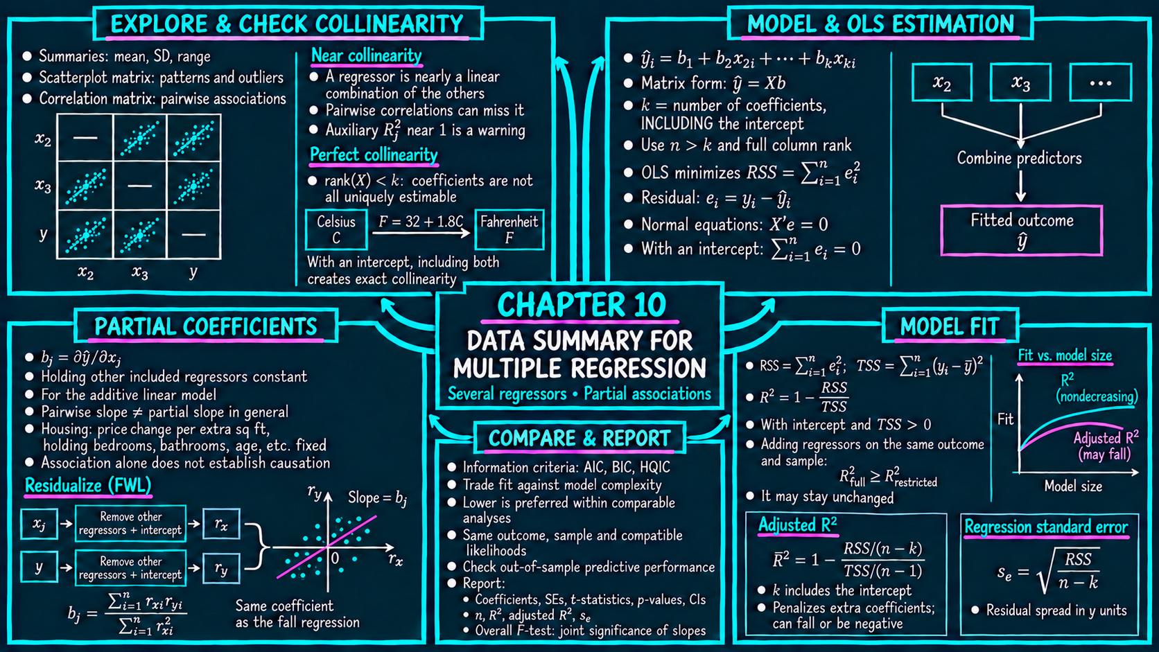
<img src="https://raw.githubusercontent.com/quarcs-lab/metricsai/main/images/ch10_visual_summary_v2.png" alt="Chapter 10 Visual Summary" width="100%">
This notebook provides an interactive introduction to multiple regression analysis. You'll learn how to work with multiple explanatory variables, interpret partial effects, assess model fit, and detect multicollinearity. All code runs directly in Google Colab without any local setup.
[](https://colab.research.google.com/github/quarcs-lab/metricsai/blob/main/notebooks_colab/ch10_Data_Summary_for_Multiple_Regression.ipynb)
<div class="chapter-resources">
<a href="https://www.youtube.com/watch?v=9398KshS_JA" target="_blank" class="resource-btn">🎬 AI Video</a>
<a href="https://quarcs-lab.github.io/metricsai/slides/ch10/index.html" target="_blank" class="resource-btn">🧑🏽🏫 Mendez Slides</a>
<a href="https://quarcs-lab.github.io/metricsai/slides/ch10/cameron_slides_ch10.pdf" target="_blank" class="resource-btn">📊 Cameron Slides</a>
<a href="https://quarcs-lab.github.io/metricsai/quizzes/ch10.html" target="_blank" class="resource-btn">✏️ Quiz</a>
<a href="https://gemini.google.com/gem/1mvbUPJb9CZ1SEWlxui86i25-HINaUH1c?usp=sharing" target="_blank" class="resource-btn">🤖 AI Tutor</a>
</div>
## Chapter Overview
This chapter extends bivariate regression to the more realistic case where we want to predict an outcome using **multiple explanatory variables** simultaneously. Multiple regression allows us to estimate the partial effect of each variable while controlling for others—a crucial feature for empirical economic analysis.
**What you'll learn:**
- Extend bivariate regression concepts to multiple regression with several regressors
- Interpret pairwise correlations and use them for exploratory data analysis
- Understand the ordinary least squares (OLS) method for multiple regression
- Interpret partial effects: how one regressor affects $y$ while holding others constant
- Distinguish between partial effects and total effects
- Evaluate model fit using R-squared and adjusted R-squared
- Understand information criteria (AIC, BIC) for model selection
- Recognize when regression coefficients cannot be estimated (perfect collinearity)
**Dataset used:**
- **AED_HOUSE.DTA**: 29 houses sold in Davis, California (1999) with price, size, bedrooms, bathrooms, lot size, age, and month sold
**Key economic question:**
What is the effect of house size on price **after controlling** for other characteristics like bedrooms, bathrooms, and age?
**Chapter outline:**
- 10.1 Example - House Price and Characteristics
- 10.2 Two-Way Scatterplots
- 10.3 Correlation Analysis
- 10.4 Multiple Regression Estimation
- 10.5 Partial Effects - The FWL Theorem
- 10.6 Model Fit Statistics
- 10.7 Model Comparison
- 10.8 Inestimable Models and Multicollinearity
- Key Takeaways
- Practice Exercises
- Case Studies
## Key Concepts
Six core ideas anchor this chapter. Skim them before you start, and come back when a term feels fuzzy. Each entry pairs a concrete example using the chapter's data with a non-technical analogy. Click a panel to expand it.
**Multiple Regression Model:** A regression with two or more explanatory variables, $\hat{y} = b_1 + b_2 x_2 + b_3 x_3 + \cdots + b_k x_k$. Unlike bivariate regression, each slope $b_j$ is a *partial* coefficient — it isolates the effect of $x_j$ on $y$ while statistically holding the other regressors fixed.
::::: {.columns}
:::: {.column width="50%"}
::: {.callout-tip collapse="true" appearance="simple" title="Example"}
For the 29 Davis houses, the chapter fits $\widehat{\text{price}} = b_1 + b_2 \cdot \text{size} + b_3 \cdot \text{bedrooms} + b_4 \cdot \text{bathrooms} + b_5 \cdot \text{lotsize} + b_6 \cdot \text{age} + b_7 \cdot \text{monthsold}$. The estimated `size` coefficient is \$68.37/sq ft (down from \$73.77 in the bivariate version) — a partial effect that excludes the influence of bedrooms, bathrooms, and the rest.
:::
::::
:::: {.column width="50%"}
::: {.callout-note collapse="true" appearance="simple" title="Analogy"}
An orchestra plays a chord: the cello, viola, and violin all sound at once. Bivariate regression listens to one instrument as if it were the whole sound. Multiple regression is a sound engineer's *isolation track* — turning each instrument up against a backdrop of the others, so you hear what that one instrument adds on its own.
:::
::::
:::::
**Pairwise Correlation Matrix:** A square table whose $(i, j)$ entry is the correlation $r_{x_i x_j}$ between two columns of the dataset. It is the standard exploratory tool before fitting multiple regression — strong off-diagonal correlations signal candidate predictors *and* warn of likely multicollinearity.
::::: {.columns}
:::: {.column width="50%"}
::: {.callout-tip collapse="true" appearance="simple" title="Example"}
The chapter's correlation matrix on the Davis houses shows $r(\text{price}, \text{size}) = 0.79$ (the strongest predictor) and $r(\text{price}, \text{bedrooms}) = 0.43$. It also flags $r(\text{size}, \text{bedrooms}) = 0.52$ — a moderate inter-regressor correlation that explains why the bedrooms coefficient drops from \$23{,}667 in the bivariate fit to just \$1{,}553 once size is in the model.
:::
::::
:::: {.column width="50%"}
::: {.callout-note collapse="true" appearance="simple" title="Analogy"}
A wedding seating chart records, for every pair of guests, how well they get along. A pairwise correlation matrix is the same idea applied to data columns: for every pair of variables, one number summarising how often they "show up together". Strong pairs sit close; weak pairs go to opposite ends of the room.
:::
::::
:::::
**Control Variable:** A regressor included in the model not because it is the main quantity of interest but to prevent its omission from biasing the focal coefficient. By adding the control, the regression isolates the partial effect of the focal variable while "holding the control fixed".
::::: {.columns}
:::: {.column width="50%"}
::: {.callout-tip collapse="true" appearance="simple" title="Example"}
In the Davis house regression, `bedrooms` looks like a strong predictor of `price` on its own (\$23{,}667 per bedroom). Once `size` is added as a control variable, the bedrooms coefficient collapses to \$1{,}553 — most of the apparent bedrooms effect was really houses with more bedrooms being bigger. `size` here is a textbook control: not the "treatment" of interest but essential for an honest estimate of bedrooms.
:::
::::
:::: {.column width="50%"}
::: {.callout-note collapse="true" appearance="simple" title="Analogy"}
A laboratory experiment on plant growth holds *temperature* constant in every sample so the researcher can isolate the effect of fertiliser. Temperature is the lab's control variable — not the thing being studied, but the thing being kept fixed so the rest of the comparison is fair. In regression, control variables play the same role with statistical instead of physical fixing.
:::
::::
:::::
**Confounder:** A variable that influences both the focal regressor and the outcome, creating an indirect channel through which the focal regressor *appears* to affect $y$ even when it does not. Including the confounder as a control variable typically shrinks (or flips) the focal coefficient toward its true partial effect.
::::: {.columns}
:::: {.column width="50%"}
::: {.callout-tip collapse="true" appearance="simple" title="Example"}
For the Davis houses, `size` is a confounder of the bedrooms–price relationship: bigger houses tend to have more bedrooms *and* fetch higher prices. That is why omitting `size` made bedrooms look like a \$23{,}667-per-room driver, while including it brought the partial effect down to \$1{,}553 — most of the original bedrooms coefficient was really `size` showing up in disguise.
:::
::::
:::: {.column width="50%"}
::: {.callout-note collapse="true" appearance="simple" title="Analogy"}
Across cities, ice-cream sales and drowning deaths are tightly correlated — but ice cream isn't drowning anyone. Summer is the confounder: it raises both sales and water-park traffic. Failing to control for the season makes ice cream look like a killer; controlling for it reveals the spurious link, just as `size` reveals bedrooms' inflated coefficient.
:::
::::
:::::
**Adjusted $R^2$:** A version of $R^2$ that penalises for the number of regressors: $\bar{R}^2 = 1 - \frac{\text{RSS}/(n-k)}{\text{TSS}/(n-1)}$. Adding a useless variable never decreases plain $R^2$ but typically lowers $\bar{R}^2$ — making it the better fit metric when comparing models of different sizes.
::::: {.columns}
:::: {.column width="50%"}
::: {.callout-tip collapse="true" appearance="simple" title="Example"}
For the Davis houses, the simple regression on `size` alone gives $R^2 = 0.617$ and $\bar{R}^2 = 0.603$. The full model with all six regressors raises $R^2$ to $0.651$ — but $\bar{R}^2$ actually *falls* to $0.555$. Plain $R^2$ rewards extra variables; adjusted $R^2$ recognises that the extras barely earned their keep on only $n = 29$ observations.
:::
::::
:::: {.column width="50%"}
::: {.callout-note collapse="true" appearance="simple" title="Analogy"}
A football league lets teams sign extra players, but charges a salary-cap penalty for each one. A team with twenty players might score slightly more goals (raw $R^2$ rises), yet still finish the season worse off after paying the penalty (adjusted $R^2$ falls). Adjusted $R^2$ is the league's way of asking, "did those extra signings *really* help?"
:::
::::
:::::
**Perfect Collinearity:** The situation where one regressor is an exact linear combination of others (e.g., `size_twice = 2 × size`). When this happens, the OLS normal equations have no unique solution — software either drops a regressor automatically or returns an error.
::::: {.columns}
:::: {.column width="50%"}
::: {.callout-tip collapse="true" appearance="simple" title="Example"}
The chapter constructs `size_twice = 2 × size` and tries to estimate `price ~ size + size_twice + bedrooms`. Because `size_twice` adds *no* new information beyond `size`, the regression is inestimable: the software drops one of the two collinear variables (pyfixest prints a warning naming it) and reports the rest. In contrast, the actual six predictors in the Davis dataset show only moderate VIFs, so all six can be estimated jointly.
:::
::::
:::: {.column width="50%"}
::: {.callout-note collapse="true" appearance="simple" title="Analogy"}
Identical twins walk into a tailor's shop wanting matching suits. The tailor has one set of measurements but two customers — there is no way to assign a "different" credit-card to each twin from the dataset alone, because the two are indistinguishable. Perfect collinearity is OLS facing identical twins among its regressors: distinct names, identical information.
:::
::::
:::::
## Setup
First, we import the necessary Python packages and configure the environment for reproducibility. All data will stream directly from GitHub.
```{python}
#| code-fold: true
#| code-summary: "Setup: Import libraries and configure environment"
# --- Libraries ---
import numpy as np                        # numerical operations
import pandas as pd                       # data manipulation
import matplotlib.pyplot as plt           # plotting
import seaborn as sns                     # statistical visualization
import pyfixest as pf                     # fast estimation with robust SEs
from scipy import stats                   # statistical distributions
import random
import os

# --- Reproducibility ---
RANDOM_SEED = 42
random.seed(RANDOM_SEED)
np.random.seed(RANDOM_SEED)
os.environ['PYTHONHASHSEED'] = str(RANDOM_SEED)

# --- Data source ---
GITHUB_DATA_URL = "https://raw.githubusercontent.com/quarcs-lab/data-open/master/AED/"

# --- Plotting style (dark theme matching book design) ---
plt.style.use('dark_background')
sns.set_style("darkgrid")
plt.rcParams.update({
    'axes.facecolor': '#1a2235',
    'figure.facecolor': '#12162c',
    'grid.color': '#3a4a6b',
    'figure.figsize': (10, 6),
    'text.color': 'white',
    'axes.labelcolor': 'white',
    'xtick.color': 'white',
    'ytick.color': 'white',
    'axes.edgecolor': '#1a2235',
})

print("Setup complete! Ready to analyze house price data.")
```
## 10.1 Example - House Price and Characteristics
We begin with a real estate dataset from Davis, California. Understanding house prices is a classic economic application because prices reflect both fundamental characteristics (size, bedrooms) and market conditions.
**The dataset contains:**
- **Price**: Sale price in dollars
- **Size**: House size in square feet
- **Bedrooms**: Number of bedrooms
- **Bathrooms**: Number of bathrooms
- **Lotsize**: Size of lot (1=small, 2=medium, 3=large)
- **Age**: House age in years
- **Monthsold**: Month of year house was sold
**Economic motivation:** A simple regression of price on bedrooms might find a positive relationship, but is this because bedrooms directly add value, or because houses with more bedrooms tend to be larger? Multiple regression helps us disentangle these effects.
The code below loads the dataset from GitHub and displays the first ten observations together with summary statistics. Check each variable's scale and range — price is in dollars, size in square feet — before we start modeling.
```{python}
# Load house price data
data_house = pd.read_stata(GITHUB_DATA_URL + 'AED_HOUSE.DTA')

# Display first few observations
print("First 10 observations:")
print(data_house[['price', 'size', 'bedrooms', 'bathrooms', 'lotsize', 'age', 'monthsold']].head(10))

# Display data summary
print("\nSummary statistics:")
data_house.describe()
```
**Interpreting the summary statistics:** The 29 Davis houses sold for an average of about \$253,910 (ranging from \$204,000 to \$375,000) and average about 1,883 square feet, with 3.8 bedrooms and 2.2 bathrooms; the typical house is about 36 years old. Keep this small sample size in mind — with only 29 observations, coefficients on six regressors will be imprecisely estimated.
### Bivariate vs. Multiple Regression
Let's compare a simple regression (price on bedrooms only) with a multiple regression (price on bedrooms AND size). This illustrates how controlling for other variables changes coefficient estimates.
**Key insight:** In the bivariate regression, the bedrooms coefficient captures both the direct effect of bedrooms and the indirect effect through correlation with size. In multiple regression, we isolate the **partial effect** of bedrooms holding size constant.
```{python}
# Bivariate regression: price ~ bedrooms
model_bivariate = pf.feols('price ~ bedrooms', data=data_house)

# Key results: bivariate
print(f"Bivariate: bedrooms coef = ${model_bivariate.coef()['bedrooms']:,.2f}, R² = {model_bivariate._r2:.4f}")

# Full regression output
model_bivariate.summary()

# Multiple regression: price ~ bedrooms + size
model_multiple = pf.feols('price ~ bedrooms + size', data=data_house)

# Key results: multiple
print(f"Multiple: bedrooms coef = ${model_multiple.coef()['bedrooms']:,.2f}, R² = {model_multiple._r2:.4f}")

# Full regression output
model_multiple.summary()

# Compare bedrooms coefficient
# COEFFICIENT COMPARISON
print(f"Bedrooms coefficient (bivariate):  ${model_bivariate.coef()['bedrooms']:,.2f}")
print(f"Bedrooms coefficient (multiple):   ${model_multiple.coef()['bedrooms']:,.2f}")
print(f"Change: ${model_multiple.coef()['bedrooms'] - model_bivariate.coef()['bedrooms']:,.2f}")
```
> **Key Concept 10.1: Partial Effects vs. Total Effects in Multiple Regression**
>
> In bivariate regression, the bedrooms coefficient (\$23,667) captures both the direct effect of bedrooms and the indirect effect through correlation with size. In multiple regression, the bedrooms coefficient drops to \$1,553 — the **partial effect** holding size constant — and is no longer statistically significant ($t = 0.20$, $p = 0.84$). This dramatic change illustrates why controlling for confounders is essential for isolating individual variable effects.
## 10.2 Two-Way Scatterplots
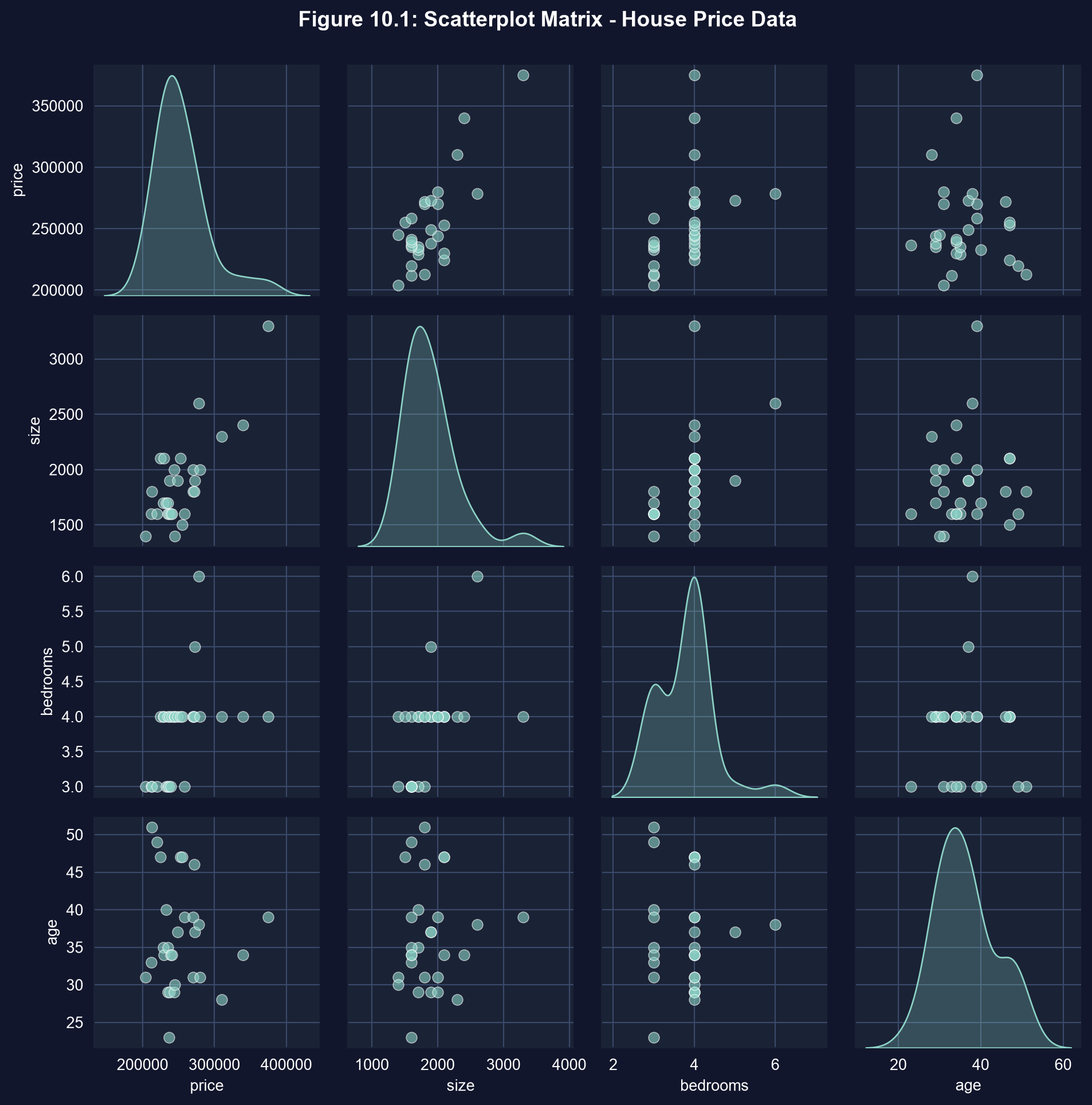
Before running multiple regression, it's useful to visualize pairwise relationships between variables. A **scatterplot matrix** shows all two-way scatterplots simultaneously.
**What to look for:**
- Strong linear relationships (potential predictors of price)
- Correlation between explanatory variables (potential multicollinearity)
- Outliers or non-linear patterns
The diagonal shows the distribution of each variable using kernel density estimates (KDE).
```{python}
# Create scatterplot matrix
plot_vars = ['price', 'size', 'bedrooms', 'age']
g = sns.pairplot(data_house[plot_vars], diag_kind='kde',
                 plot_kws={'alpha': 0.6, 's': 50})  # alpha = transparency, s = marker size
g.fig.suptitle('Figure 10.1: Scatterplot Matrix - House Price Data',
               fontsize=14, fontweight='bold', y=1.00)
plt.tight_layout()
plt.show()

print("Scatterplot matrix created.")
print("Notice: Price shows strongest relationship with Size.")
```
> **Key Concept 10.2: Exploratory Data Analysis with Scatterplot Matrices**
>
> Pairwise scatterplot matrices display all two-way relationships simultaneously, revealing linear associations, nonlinearities, clusters, and outliers before formal modeling. They also highlight potential multicollinearity: if two regressors are correlated (e.g., size and bedrooms, with a moderate $r = 0.52$), their individual effects may be hard to separate in a regression.
## 10.3 Correlation Analysis
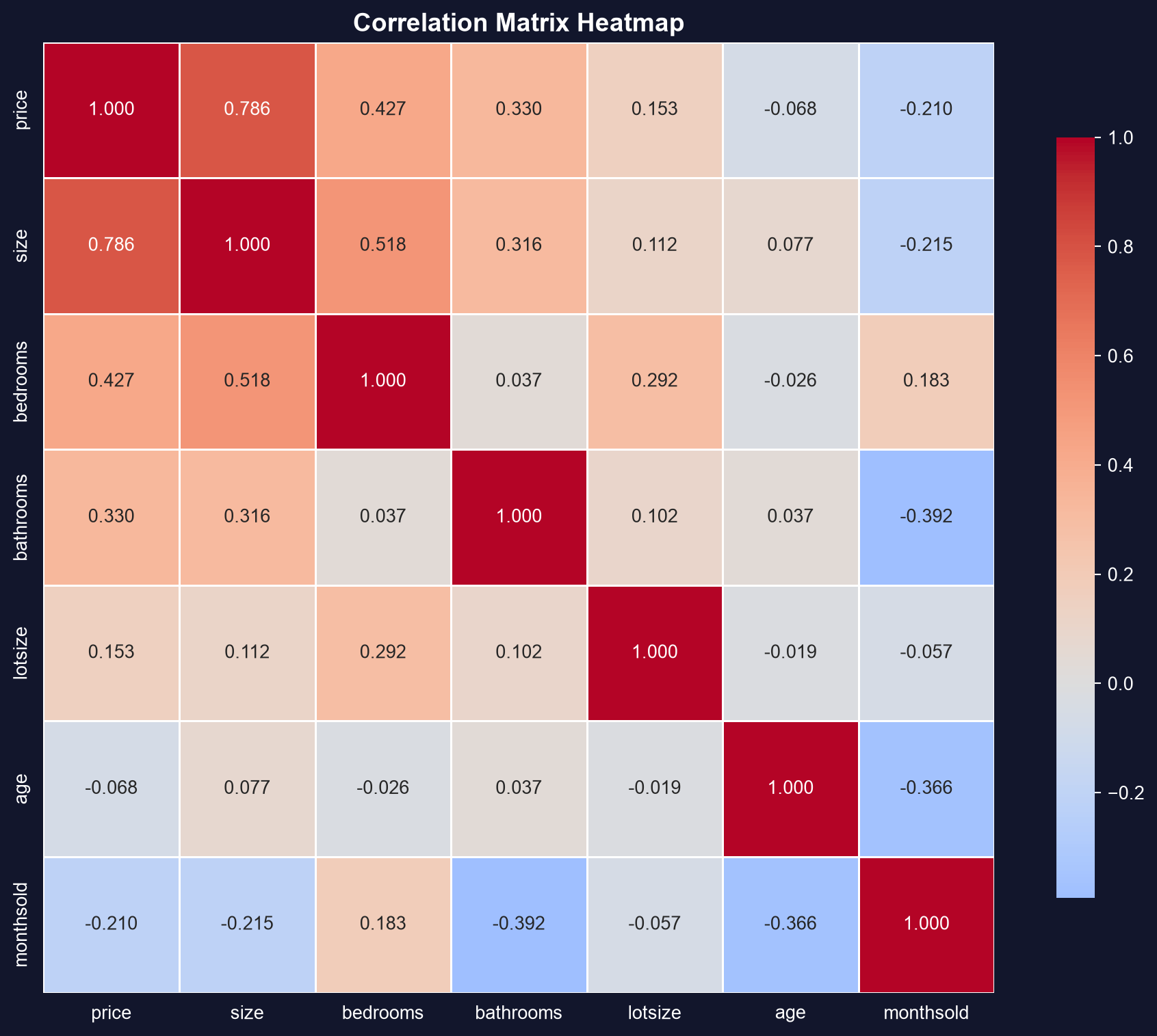
The **correlation coefficient** measures the strength of linear association between two variables, ranging from -1 (perfect negative) to +1 (perfect positive).
**Correlation matrix insights:**
- **Price is most correlated with Size** (r = 0.79), then Bedrooms (r = 0.43)
- **Size and Bedrooms are correlated** (r = 0.52), which can cause multicollinearity
- Correlation ≠ causation (merely shows association)
A correlation heatmap provides visual representation with color intensity showing strength of correlation.
```{python}
# Calculate correlation matrix
corr_vars = ['price', 'size', 'bedrooms', 'bathrooms', 'lotsize', 'age', 'monthsold']
corr_matrix = data_house[corr_vars].corr()

print("Correlation Matrix:")
print(corr_matrix.round(3))

# Visualize correlation matrix as heatmap
fig, ax = plt.subplots(figsize=(10, 8))
sns.heatmap(corr_matrix, annot=True, fmt='.3f', cmap='coolwarm', center=0,
            square=True, linewidths=1, cbar_kws={"shrink": 0.8})
ax.set_title('Correlation Matrix Heatmap', fontsize=14, fontweight='bold')
plt.tight_layout()
plt.show()

print(f"Price-Size correlation: {corr_matrix.loc['price', 'size']:.3f}")
print(f"Size-Bedrooms correlation: {corr_matrix.loc['size', 'bedrooms']:.3f}")
```
> **Key Concept 10.3: Correlation vs. Causation in Multivariate Analysis**
>
> High bivariate correlation (e.g., bedrooms-price, $r = 0.43$) may diminish or vanish after controlling for confounders. In our data, bedrooms correlate with price largely because bigger houses have more bedrooms. Multiple regression isolates each variable's partial contribution, revealing that size — not bedrooms — accounts for most of the price variation.
## 10.4 Multiple Regression Estimation
Now we estimate the **full multiple regression model** with all available predictors. The regression equation is:
$$\widehat{\text{price}} = b_1 + b_2 \times \text{size} + b_3 \times \text{bedrooms} + b_4 \times \text{bathrooms} + b_5 \times \text{lotsize} + b_6 \times \text{age} + b_7 \times \text{monthsold}$$
**Ordinary Least Squares (OLS)** chooses coefficients $b_1, ..., b_7$ to minimize the sum of squared residuals:
$$\min \sum_{i=1}^{n} (y_i - \widehat{y}_i)^2$$
where $y_i$ is the actual price and $\widehat{y}_i$ is the predicted price.
```{python}
# Estimate full multiple regression model
model_full = pf.feols('price ~ size + bedrooms + bathrooms + lotsize + age + monthsold', data=data_house)

# Key results
r_squared_full = model_full._r2
adj_r_squared_full = model_full._adj_r2
size_coef = model_full.coef()['size']

print(f"Estimated equation: price = {model_full.coef()['Intercept']:,.0f} + {size_coef:.2f} x size + ...")
print(f"Size effect: each additional sq ft is associated with ${size_coef:,.2f} higher price")
print(f"R-squared: {r_squared_full:.4f} ({r_squared_full*100:.1f}% of variation explained)")
print(f"Adjusted R-squared: {adj_r_squared_full:.4f}")

# Full regression output
model_full.summary()
```
### Coefficient Interpretation with Confidence Intervals
Each regression coefficient represents a **partial effect**: the expected change in price when that variable increases by one unit, **holding all other variables constant**.
**Example interpretation (Size coefficient):**
- Coefficient ≈ \$68.37 per square foot
- Interpretation: A one square foot increase in house size is associated with a \$68.37 increase in price, holding bedrooms, bathrooms, lot size, age, and month sold constant.
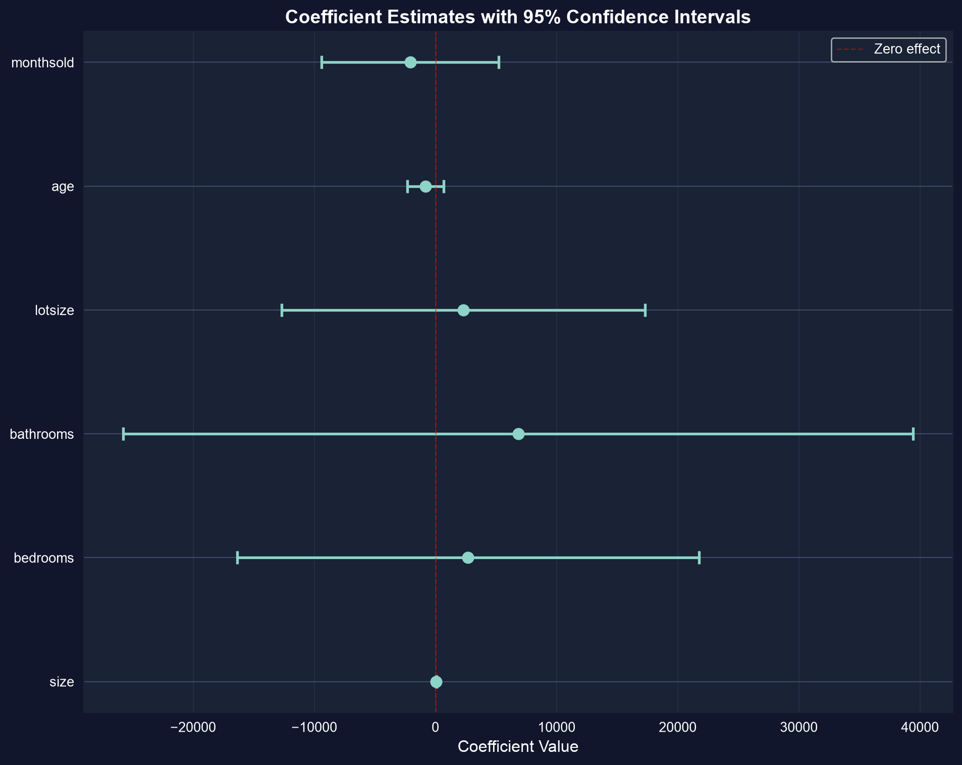
- Significance: This effect is statistically significant ($t = 4.44$, $p < 0.001$) — size is the only regressor whose 95% confidence interval excludes zero.
The 95% confidence interval tells us the range of plausible values for each coefficient. Throughout this chapter we report classical (homoskedasticity-assuming) standard errors, as AED does before Chapter 12; Chapter 12 introduces heteroskedasticity-robust standard errors, which are preferred in practice.
```{python}
# Display coefficients with 95% confidence intervals
conf_int = model_full.confint()
coef_table = pd.DataFrame({
    'Coefficient': model_full.coef(),
    'Std. Error': model_full.se(),
    'CI Lower': conf_int.iloc[:, 0],
    'CI Upper': conf_int.iloc[:, 1],
    't-statistic': model_full.tstat(),
    'p-value': model_full.pvalue()
})

print("Coefficients with 95% Confidence Intervals:")
coef_table

# Size is the only statistically significant predictor (p < 0.05)
```
**Interpreting the table:** Size is the only statistically significant predictor (t = 4.44, p < 0.001), with a 95% confidence interval of roughly \$36 to \$100 per square foot. Every other coefficient has a confidence interval that comfortably includes zero — once size is controlled for, bedrooms, bathrooms, lot size, age, and month sold add little explanatory power in this small sample.
> **Key Concept 10.4: Interpreting Partial Effects in Multiple Regression**
>
> Each coefficient $b_j$ measures the expected change in $y$ when $x_j$ increases by one unit, **holding all other regressors constant**. For example, a size coefficient of \$68.37 means each additional square foot is associated with a \$68.37 price increase, controlling for bedrooms, bathrooms, lot size, age, and month sold. Statistical significance is assessed through confidence intervals and $t$-tests.
## 10.5 Partial Effects - The FWL Theorem
The **Frisch-Waugh-Lovell (FWL) Theorem** states that the coefficient on any variable in multiple regression equals the coefficient from a bivariate regression of $y$ on the **residualized** version of that variable.
**Demonstration:**
1. Regress `size` on all other variables, obtain residuals $\widetilde{\text{size}}$
2. Regress `price` on $\widetilde{\text{size}}$ only
3. The coefficient will exactly match the `size` coefficient from the full multiple regression
**Intuition:** The residual $\widetilde{\text{size}}$ represents the variation in size that is **not explained** by other variables. This is why multiple regression isolates partial effects.
```{python}
# Step 1: Regress size on all other variables
model_size_on_others = pf.feols('size ~ bedrooms + bathrooms + lotsize + age + monthsold', data=data_house)
resid_size = model_size_on_others._u_hat

# Step 2: Regress price on residualized size
data_house['resid_size'] = resid_size
model_price_on_resid = pf.feols('price ~ resid_size', data=data_house)

# Compare coefficients
# DEMONSTRATION: FWL THEOREM (Partial Effects)
print(f"Size coefficient from FULL multiple regression:  {model_full.coef()['size']:.10f}")
print(f"Coefficient on residualized size (bivariate):    {model_price_on_resid.coef()['resid_size']:.10f}")
print(f"Difference (numerical precision):                 {abs(model_full.coef()['size'] - model_price_on_resid.coef()['resid_size']):.15f}")
```
> **Key Concept 10.5: The Frisch-Waugh-Lovell (FWL) Theorem**
>
> The partial effect of $x_j$ in a multiple regression equals the slope from a bivariate regression of $y$ on $\widetilde{x}_j$, where $\widetilde{x}_j$ is the residual from regressing $x_j$ on all other regressors. Intuitively, $\widetilde{x}_j$ captures the variation in $x_j$ that is independent of the other variables — this is exactly what multiple regression uses to estimate partial effects.
## 10.6 Model Fit Statistics
Several statistics summarize how well the regression model fits the data:
**R-squared ($R^2$):**
- Fraction of variation in $y$ explained by the regressors
- Formula: $R^2 = \frac{\text{Explained SS}}{\text{Total SS}} = 1 - \frac{\text{Residual SS}}{\text{Total SS}}$
- Range: 0 to 1 (higher is better fit)
- **Problem:** Never decreases when adding variables (even irrelevant ones)
**Adjusted R-squared ($\bar{R}^2$):**
- Penalizes model complexity (number of parameters $k$)
- Formula: $\bar{R}^2 = 1 - \frac{\text{RSS}/(n-k)}{\text{TSS}/(n-1)}$
- Can decrease when adding unhelpful variables
- Preferred for model comparison
**Root MSE (Standard error of regression):**
- Typical size of prediction error
- Formula: $s_e = \sqrt{\frac{1}{n-k}\sum (y_i - \widehat{y}_i)^2}$
- Same units as $y$ (dollars in our case)
- Note: the `RMSE` printed in pyfixest summaries divides by $n$ rather than $n-k$, so it is slightly smaller than $s_e$
```{python}
# Calculate and display model fit statistics
n = len(data_house)
k = len(model_full.coef())  # includes intercept
df = n - k

# MODEL FIT STATISTICS
print(f"Sample size (n):               {n}")
print(f"Number of parameters (k):      {k}")
print(f"Degrees of freedom (n-k):      {df}")
print(f"\nR-squared:                     {model_full._r2:.6f}")
print(f"Adjusted R-squared:            {model_full._adj_r2:.6f}")
print(f"Root MSE:                      ${np.sqrt(np.sum(model_full._u_hat**2) / (int(model_full._N) - len(model_full.coef()))):,.2f}")

# Verify R² = [Corr(y, ŷ)]²
predicted = model_full.predict()
corr_y_yhat = np.corrcoef(data_house['price'], predicted)[0, 1]
print(f"\nVerification: R² = [Corr(y, ŷ)]²")
print(f"  Correlation(y, ŷ):           {corr_y_yhat:.6f}")
print(f"  [Correlation(y, ŷ)]²:        {corr_y_yhat**2:.6f}")
print(f"  R² from model:                {model_full._r2:.6f}")
print(f"  Match: {np.isclose(corr_y_yhat**2, model_full._r2)}")
```
**Interpreting the fit statistics:** The six regressors explain about 65% of the variation in price, but the adjusted $R^2$ of 0.555 reveals that much of that gain is a mechanical reward for adding variables. The Root MSE of roughly \$24,936 is the typical prediction error — sizable relative to an average price of about \$253,910. The verification confirms that $R^2$ equals the squared correlation between actual and fitted prices.
### Information Criteria (AIC and BIC)
**Akaike Information Criterion (AIC)** and **Bayesian Information Criterion (BIC)** are more sophisticated measures that penalize model complexity:
$$\text{AIC} = n \times \ln(\widehat{\sigma}_e^2) + n(1 + \ln 2\pi) + 2k$$
$$\text{BIC} = n \times \ln(\widehat{\sigma}_e^2) + n(1 + \ln 2\pi) + k \times \ln(n)$$
where $\widehat{\sigma}_e^2 = \text{RSS}/n$ (note the divisor is $n$, not the $n-k$ used for $s_e$).
**Key points:**
- **Lower values are better** (unlike R²)
- BIC penalizes complexity more heavily than AIC
- Useful for comparing non-nested models
- Different software packages may use different conventions (scaling by $n$)
```{python}
# Calculate information criteria
# INFORMATION CRITERIA

# Manual calculation of AIC and BIC (Stata convention)
rss = np.sum(model_full._u_hat ** 2)
aic_stata = n * np.log(rss/n) + n * (1 + np.log(2*np.pi)) + 2*k
bic_stata = n * np.log(rss/n) + n * (1 + np.log(2*np.pi)) + k*np.log(n)

print(f"AIC (Stata convention):        {aic_stata:.4f}")
print(f"BIC (Stata convention):        {bic_stata:.4f}")
```
> **Key Concept 10.6: Model Selection with Adjusted R-squared vs. Information Criteria**
>
> Adjusted $R^2$ penalizes complexity mildly by dividing sums of squares by degrees of freedom. Information criteria (AIC, BIC) impose stronger penalties: BIC = $n \ln(\hat{\sigma}_e^2) + k \ln(n)$ (omitting a constant that does not affect model comparisons). Smaller AIC/BIC values indicate better models. BIC is generally preferred because its penalty grows with sample size, favoring more parsimonious specifications.
## 10.7 Model Comparison
It's often useful to compare multiple model specifications side-by-side. Here we compare:
- **Simple model:** Price predicted by size only
- **Full model:** Price predicted by all variables
**Key comparison points:**
- How much does R² improve?
- Does adjusted R² improve (accounting for added complexity)?
- How do coefficient estimates change?
**Economic interpretation:** If adding 5 more variables only modestly improves fit, the simple model may be preferred (parsimony principle).
```{python}
# Estimate simple model (size only)
model_simple = pf.feols('price ~ size', data=data_house)

# Information criteria (Stata convention). pyfixest's Feols has no ._aic/._bic,
# so compute them from each model's residual sum of squares.
def stata_ic(model):
    n_obs = int(model._N)
    n_par = len(model.coef())
    rss_m = np.sum(model._u_hat ** 2)
    const = n_obs * (1 + np.log(2 * np.pi))
    aic = n_obs * np.log(rss_m / n_obs) + const + 2 * n_par
    bic = n_obs * np.log(rss_m / n_obs) + const + n_par * np.log(n_obs)
    return aic, bic

aic_simple, bic_simple = stata_ic(model_simple)
aic_full, bic_full = stata_ic(model_full)

# Create comparison table
# MODEL COMPARISON: Simple vs. Full

comparison_stats = pd.DataFrame({
    'Model': ['Simple (size only)', 'Full (all variables)'],
    'R²': [model_simple._r2, model_full._r2],
    'Adj R²': [model_simple._adj_r2, model_full._adj_r2],
    'AIC': [aic_simple, aic_full],
    'BIC': [bic_simple, bic_full],
    'N': [n, n]
})

print(comparison_stats.to_string(index=False))

print(f"R² increases from {model_simple._r2:.3f} to {model_full._r2:.3f}")
print(f"Adj R² decreases from {model_simple._adj_r2:.3f} to {model_full._adj_r2:.3f}")
```
> **Key Concept 10.7: The Parsimony Principle**
>
> Simpler models are preferred unless additional variables meaningfully improve fit. In our house price example, adding five variables beyond size barely increased $R^2$ (0.617 $\to$ 0.651) while adjusted $R^2$ actually fell (0.603 $\to$ 0.555). Check adjusted $R^2$, AIC, and BIC — if they don't improve, the simpler model is preferred.
## 10.8 Inestimable Models and Multicollinearity
**Perfect multicollinearity** occurs when one regressor is an exact linear combination of others. In this case, OLS cannot estimate all coefficients (the model is "inestimable").
**Example:** If we create `size_twice = 2 × size` and include both `size` and `size_twice` as regressors, the model is perfectly collinear.
**Variance Inflation Factor (VIF)** detects multicollinearity:
- VIF measures how much a variable's variance is inflated due to correlation with other regressors
- Formula: $VIF_j = \frac{1}{1 - R_j^2}$ where $R_j^2$ is from regressing $x_j$ on all other $x$'s
- **Rule of thumb:** VIF > 10 indicates problematic multicollinearity
**Consequences of high multicollinearity:**
- Large standard errors (imprecise estimates)
- Unstable coefficients (small data changes → big estimate changes)
- Difficulty interpreting individual effects
```{python}
# Demonstrate perfect multicollinearity
# DEMONSTRATION: Perfect Multicollinearity

# Create a perfectly collinear variable
data_house['size_twice'] = 2 * data_house['size']

print("Creating variable: size_twice = 2 × size")
print("Attempting to estimate: price ~ size + size_twice + bedrooms\n")

try:
    model_collinear = pf.feols('price ~ size + size_twice + bedrooms', data=data_house)
    print("Model estimated (software automatically dropped one variable):")
    model_collinear.summary()
except Exception as e:
    print(f"Error: {type(e).__name__}")
    print(f"Message: {str(e)}")
```
**Interpreting the output:** pyfixest warns that `size_twice` was dropped due to multicollinearity — it carries no information beyond `size` itself. Notice that the remaining estimates are identical to the earlier `price ~ bedrooms + size` regression: dropping the redundant regressor restores an estimable model without changing anything else.
### Variance Inflation Factors (VIF)
Now let's calculate VIF for each variable in our full model to check for multicollinearity problems.
```{python}
# Calculate VIF for each variable in the full model
from statsmodels.stats.outliers_influence import variance_inflation_factor

X = data_house[['size', 'bedrooms', 'bathrooms', 'lotsize', 'age', 'monthsold']].copy()
X.insert(0, 'const', 1.0)  # VIF requires the intercept column in the design matrix
vif_data = pd.DataFrame()
vif_data["Variable"] = X.columns[1:]
vif_data["VIF"] = [variance_inflation_factor(X.values, i) for i in range(1, X.shape[1])]

# VARIANCE INFLATION FACTORS (VIF)
print(vif_data.to_string(index=False))


max_vif = vif_data['VIF'].max()
if max_vif > 10:
    print(f"\nWarning: Maximum VIF = {max_vif:.2f} indicates multicollinearity issues.")
elif max_vif > 5:
    print(f"\nNote: Maximum VIF = {max_vif:.2f} shows moderate multicollinearity.")
else:
    print(f"\nGood: Maximum VIF = {max_vif:.2f} - no serious multicollinearity detected.")
```
> **Key Concept 10.8: Detecting Multicollinearity with VIF**
>
> The Variance Inflation Factor (VIF) quantifies how much a coefficient's variance is inflated due to correlation with other regressors. VIF$_j = 1/(1 - R_j^2)$, where $R_j^2$ is from regressing $x_j$ on all other regressors. A VIF above 5 suggests moderate concern; above 10 indicates severe multicollinearity that inflates standard errors and destabilizes estimates. Perfect collinearity (VIF $\to \infty$) makes coefficients inestimable.
### Visualization: Actual vs. Predicted Values
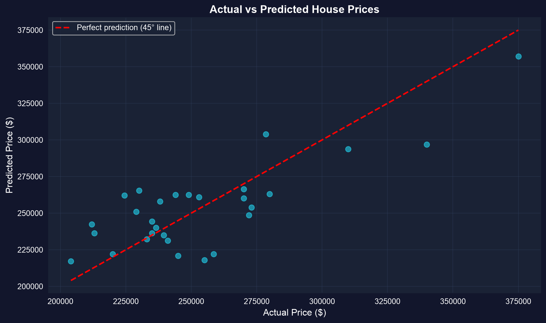
A plot of actual vs. predicted values helps visualize model fit. Points close to the 45-degree line indicate accurate predictions.
```{python}
# Create actual vs predicted plot
fig, ax = plt.subplots(figsize=(10, 6))
ax.scatter(data_house['price'], model_full.predict(), alpha=0.6, s=50, color='#22d3ee')  # alpha = transparency, s = marker size
ax.plot([data_house['price'].min(), data_house['price'].max()],
        [data_house['price'].min(), data_house['price'].max()],
        'r--', linewidth=2, label='Perfect prediction (45° line)')
ax.set_xlabel('Actual Price ($)', fontsize=12)
ax.set_ylabel('Predicted Price ($)', fontsize=12)
ax.set_title('Actual vs Predicted House Prices', fontsize=14, fontweight='bold')
ax.legend()
ax.grid(True, alpha=0.3)
plt.tight_layout()
plt.show()

print("Points close to the red line indicate accurate predictions.")
```
**What to look for in this actual vs. predicted plot:**
- **Alignment with 45-degree line**: Points close to the red dashed line indicate accurate predictions
- **Systematic deviations**: Clusters above or below the line suggest the model over- or under-predicts for certain price ranges
- **Spread**: Wider scatter around the line means larger prediction errors
### Visualization: Residual Plot
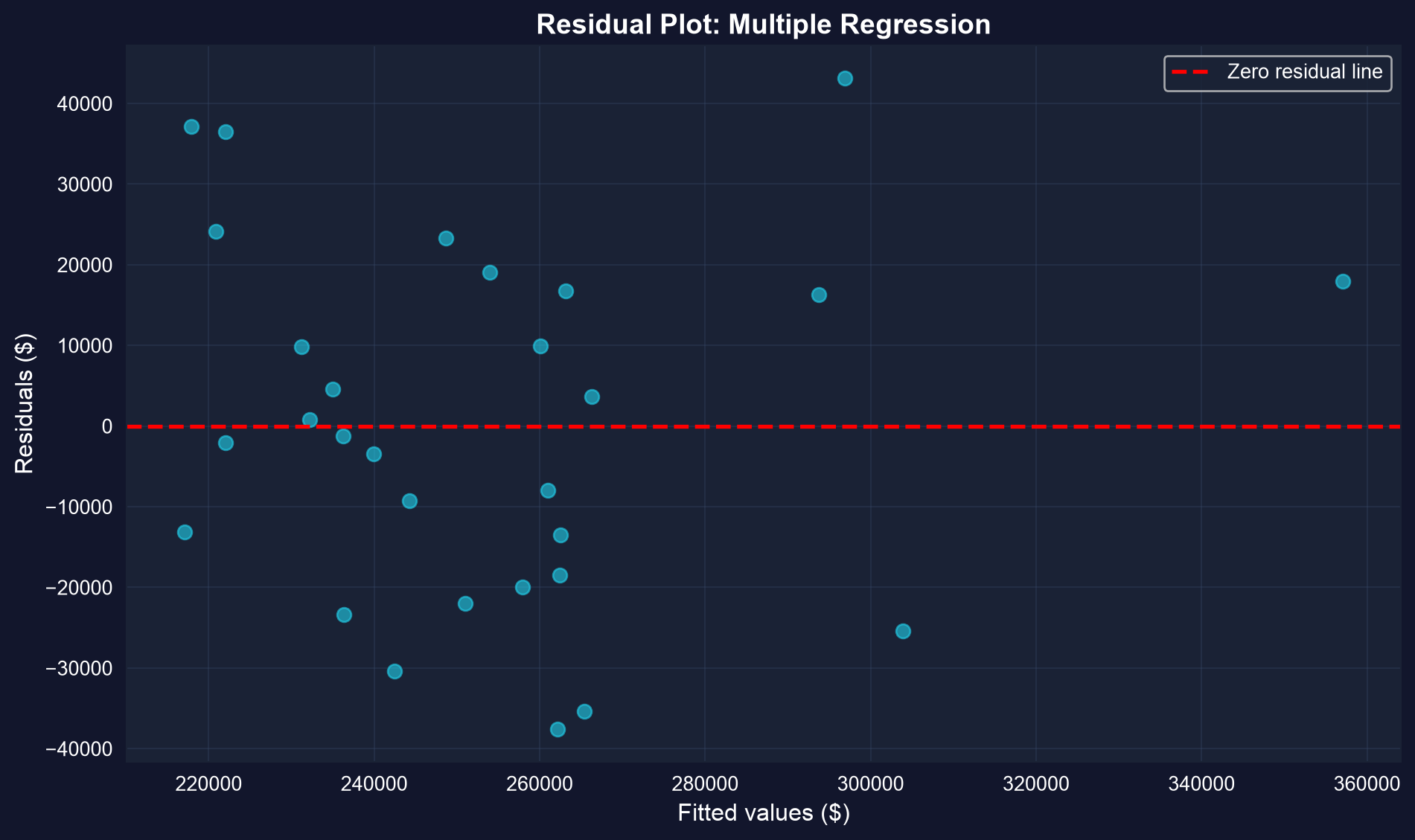
A **residual plot** (residuals vs. fitted values) helps diagnose model problems:
- **Random scatter around zero:** Good (model assumptions satisfied)
- **Patterns (curves, funnels):** Bad (model misspecification or heteroskedasticity)
- **Outliers:** Investigate unusual observations
```{python}
# Create residual plot
fig, ax = plt.subplots(figsize=(10, 6))
ax.scatter(model_full.predict(), model_full._u_hat, alpha=0.6, s=50, color='#22d3ee')  # alpha = transparency, s = marker size
ax.axhline(y=0, color='red', linestyle='--', linewidth=2, label='Zero residual line')
ax.set_xlabel('Fitted values ($)', fontsize=12)
ax.set_ylabel('Residuals ($)', fontsize=12)
ax.set_title('Residual Plot: Multiple Regression', fontsize=14, fontweight='bold')
ax.legend()
ax.grid(True, alpha=0.3)
plt.tight_layout()
plt.show()

print("Random scatter around zero suggests model assumptions are reasonable.")
```
**What to look for in this residual plot:**
- **Random scatter**: Residuals should appear randomly distributed around the zero line (no pattern)
- **Funnel shape**: A widening or narrowing pattern suggests heteroskedasticity (non-constant error variance)
- **Outliers**: Points far from the zero line may indicate unusual observations worth investigating
### Visualization: Coefficient Plot with Confidence Intervals
A **coefficient plot** displays estimated coefficients with their 95% confidence intervals. This makes it easy to see:
- Which coefficients are significantly different from zero (CI doesn't include zero)
- Relative magnitude of effects
- Precision of estimates (narrow vs. wide CIs)
```{python}
# Create coefficient plot with confidence intervals
fig, ax = plt.subplots(figsize=(10, 8))

# Exclude intercept for better visualization
params_no_int = model_full.coef()[1:]
ci_no_int = conf_int.iloc[1:, :]

y_pos = np.arange(len(params_no_int))
ax.errorbar(params_no_int.values, y_pos,
            xerr=[params_no_int.values - ci_no_int.iloc[:, 0].values,
                  ci_no_int.iloc[:, 1].values - params_no_int.values],
            fmt='o', markersize=8, capsize=5, capthick=2, linewidth=2)
ax.set_yticks(y_pos)
ax.set_yticklabels(params_no_int.index)
ax.axvline(x=0, color='red', linestyle='--', linewidth=1, alpha=0.5, label='Zero effect')
ax.set_xlabel('Coefficient Value', fontsize=12)
ax.set_title('Coefficient Estimates with 95% Confidence Intervals',
             fontsize=14, fontweight='bold')
ax.legend()
ax.grid(True, alpha=0.3, axis='x')
plt.tight_layout()
plt.show()

print("Coefficients whose CI crosses zero are not statistically significant.")
```
**What to look for in this coefficient plot:**
- **Zero crossing**: Coefficients whose error bars cross the red dashed line are not statistically significant at 5%
- **Relative magnitude**: Raw coefficients are not comparable across variables with different units — the size coefficient (\$68 per square foot) sits nearest zero on this scale, while per-unit coefficients like bathrooms look larger; yet size is the only effect estimated precisely enough for its interval to exclude zero
- **Precision**: Narrow error bars indicate more precisely estimated coefficients
## Key Takeaways
**Data Exploration and Correlation:**
- Multiple regression extends bivariate regression to include several regressors simultaneously
- Summary statistics and two-way scatterplots provide initial overview of variable relationships
- Correlation matrices reveal pairwise associations (e.g., price-size correlation of 0.79)
- Correlation can be misleading — bedrooms correlate with price, but may simply reflect house size
**OLS Estimation:**
- Multiple regression model: $\widehat{y} = b_1 + b_2 x_2 + b_3 x_3 + \cdots + b_k x_k$
- OLS minimizes the sum of squared residuals: $\min \sum (y_i - \widehat{y}_i)^2$
- The coefficient $b_j$ can be computed by bivariate regression of $y$ on $\widetilde{x}_j$ (residualized $x_j$)
**Partial Effects:**
- Each coefficient $b_j$ measures the partial effect: the change in $\widehat{y}$ when $x_j$ changes by one unit, **holding all other regressors constant**
- Partial effects differ from total effects (which allow other regressors to vary)
- OLS measures association, not causation — use careful language ("associated with")
**Model Fit:**
- $R^2$ measures the fraction of variation in $y$ explained by all regressors (0 to 1)
- Adjusted $R^2$ penalizes model complexity: can decrease when adding weak regressors
- Standard error of regression $s_e$ measures typical prediction error in units of $y$
- Example: Adding 5 regressors increased $R^2$ from 0.617 to 0.651 but decreased $\bar{R}^2$ from 0.603 to 0.555
**Information Criteria:**
- AIC and BIC penalize larger models more heavily than adjusted $R^2$
- Smaller values indicate better models
- BIC is generally preferred (stronger complexity penalty than AIC)
**Multicollinearity:**
- Perfect collinearity makes some coefficients inestimable (the software drops one of the collinear variables, as pyfixest did with `size_twice`)
- VIF detects multicollinearity: VIF > 10 indicates problematic, VIF > 5 moderate concern
- High multicollinearity inflates standard errors and makes estimates unstable
**Python Libraries and Code:**
This single code block reproduces the core workflow of Chapter 10. It is self-contained — copy it into an empty notebook and run it to review the complete pipeline from data exploration and correlation analysis through multiple regression estimation, partial effects, model comparison, and multicollinearity diagnostics.
```python
# =============================================================================
# CHAPTER 10 CHEAT SHEET: Data Summary for Multiple Regression
# =============================================================================

# --- Libraries ---
import numpy as np                                          # numerical operations
import pandas as pd                                         # data loading and manipulation
import matplotlib.pyplot as plt                             # creating plots and visualizations
import seaborn as sns                                       # statistical visualization (heatmaps, pairplots)
import pyfixest as pf                                       # fast estimation with robust SEs
from statsmodels.stats.outliers_influence import variance_inflation_factor  # multicollinearity detection

# =============================================================================
# STEP 1: Load data and explore
# =============================================================================
# pd.read_stata() reads Stata .dta files directly from a URL
url = "https://raw.githubusercontent.com/quarcs-lab/data-open/master/AED/AED_HOUSE.DTA"
data_house = pd.read_stata(url)

print(f"Dataset: {data_house.shape[0]} observations, {data_house.shape[1]} variables")
print(data_house[['price', 'size', 'bedrooms', 'bathrooms', 'lotsize', 'age']].describe().round(2))

# =============================================================================
# STEP 2: Partial effects vs. total effects — why controls matter
# =============================================================================
# Bivariate regression captures TOTAL effect (direct + indirect through size)
model_bivariate = pf.feols('price ~ bedrooms', data=data_house)

# Multiple regression isolates the PARTIAL effect (holding size constant)
model_partial = pf.feols('price ~ bedrooms + size', data=data_house)

print(f"Bedrooms coefficient (bivariate):  ${model_bivariate.coef()['bedrooms']:,.2f}")
print(f"Bedrooms coefficient (multiple):   ${model_partial.coef()['bedrooms']:,.2f}")
print(f"Change: ${model_partial.coef()['bedrooms'] - model_bivariate.coef()['bedrooms']:,.2f}")
# The coefficient drops from ~$23,667 to ~$1,553 once we control for size

# =============================================================================
# STEP 3: Correlation matrix — check pairwise associations before modeling
# =============================================================================
# High correlations between regressors signal potential multicollinearity
corr_vars = ['price', 'size', 'bedrooms', 'bathrooms', 'lotsize', 'age']
corr_matrix = data_house[corr_vars].corr()

fig, ax = plt.subplots(figsize=(10, 8))
sns.heatmap(corr_matrix, annot=True, fmt='.3f', cmap='coolwarm', center=0,
            square=True, linewidths=1)
ax.set_title('Correlation Matrix Heatmap')
plt.tight_layout()
plt.show()

print(f"Price-Size correlation: {corr_matrix.loc['price', 'size']:.3f}")
print(f"Size-Bedrooms correlation: {corr_matrix.loc['size', 'bedrooms']:.3f}")

# =============================================================================
# STEP 4: Full multiple regression — estimate partial effects
# =============================================================================
# Each coefficient measures the change in price for a one-unit change in that
# variable, holding ALL other regressors constant
model_full = pf.feols('price ~ size + bedrooms + bathrooms + lotsize + age + monthsold', data=data_house)

size_coef = model_full.coef()['size']
print(f"Size effect: each additional sq ft is associated with ${size_coef:,.2f} higher price")
print(f"R-squared: {model_full._r2:.4f} ({model_full._r2*100:.1f}% of variation explained)")
print(f"Adjusted R-squared: {model_full._adj_r2:.4f}")

# Full regression table (coefficients, std errors, t-stats, p-values)
model_full.summary()

# =============================================================================
# STEP 5: FWL theorem — how "holding constant" actually works
# =============================================================================
# Step A: Regress size on all other regressors, keep residuals
model_size_on_others = pf.feols('size ~ bedrooms + bathrooms + lotsize + age + monthsold', data=data_house)
resid_size = model_size_on_others._u_hat

# Step B: Regress price on those residuals — the slope matches the full model
data_house['resid_size'] = resid_size
model_fwl = pf.feols('price ~ resid_size', data=data_house)

print(f"Size coef from FULL regression:     {model_full.coef()['size']:.10f}")
print(f"Coef from FWL residual regression:  {model_fwl.coef()['resid_size']:.10f}")
# These are identical — the FWL theorem in action

# =============================================================================
# STEP 6: Model comparison — parsimony vs. complexity
# =============================================================================
# Compare simple (size only) vs. full model using fit statistics
model_simple = pf.feols('price ~ size', data=data_house)

# pyfixest has no ._aic/._bic; compute them (Stata convention) from each model's RSS
def stata_ic(model):
    n_obs, n_par = int(model._N), len(model.coef())
    rss_m = np.sum(model._u_hat ** 2)
    const = n_obs * (1 + np.log(2 * np.pi))
    return (n_obs * np.log(rss_m / n_obs) + const + 2 * n_par,
            n_obs * np.log(rss_m / n_obs) + const + n_par * np.log(n_obs))

comparison = pd.DataFrame({
    'Model': ['Size only', 'Full (all variables)'],
    'R²':     [model_simple._r2,     model_full._r2],
    'Adj R²': [model_simple._adj_r2, model_full._adj_r2],
    'AIC':    [stata_ic(model_simple)[0], stata_ic(model_full)[0]],
    'BIC':    [stata_ic(model_simple)[1], stata_ic(model_full)[1]],
})
print(comparison.to_string(index=False))
# Adj R² DECREASES when adding 5 weak predictors — parsimony wins

# =============================================================================
# STEP 7: VIF — detect multicollinearity
# =============================================================================
# VIF_j = 1 / (1 - R²_j), where R²_j is from regressing x_j on all other x's
# VIF > 5: moderate concern; VIF > 10: severe multicollinearity
X = data_house[['size', 'bedrooms', 'bathrooms', 'lotsize', 'age', 'monthsold']].copy()
X.insert(0, 'const', 1.0)  # VIF requires the intercept column in the design matrix
vif_data = pd.DataFrame({
    'Variable': X.columns[1:],
    'VIF': [variance_inflation_factor(X.values, i) for i in range(1, X.shape[1])]
})
print(vif_data.to_string(index=False))

# =============================================================================
# STEP 8: Diagnostics — actual vs. predicted and residual plots
# =============================================================================
# Good fit: points hug the 45° line; residuals scatter randomly around zero
fig, axes = plt.subplots(1, 2, figsize=(14, 6))

# Actual vs. predicted
axes[0].scatter(data_house['price'], model_full.predict(), alpha=0.7, s=50)
axes[0].plot([data_house['price'].min(), data_house['price'].max()],
             [data_house['price'].min(), data_house['price'].max()],
             'r--', linewidth=2, label='Perfect prediction (45° line)')
axes[0].set_xlabel('Actual Price ($)')
axes[0].set_ylabel('Predicted Price ($)')
axes[0].set_title('Actual vs Predicted')
axes[0].legend()
axes[0].grid(True, alpha=0.3)

# Residual plot
axes[1].scatter(model_full.predict(), model_full._u_hat, alpha=0.7, s=50)
axes[1].axhline(y=0, color='red', linestyle='--', linewidth=2)
axes[1].set_xlabel('Fitted Values ($)')
axes[1].set_ylabel('Residuals ($)')
axes[1].set_title('Residual Plot')
axes[1].grid(True, alpha=0.3)

plt.tight_layout()
plt.show()
```
**Try it yourself!** Copy this code into an empty Google Colab notebook and run it: [Open Colab](https://colab.research.google.com/notebooks/empty.ipynb)
**Python tools used:** `pyfixest` (feols), `statsmodels` (VIF), `seaborn` (pairplot, heatmap), `pandas` (DataFrames), `matplotlib` (coefficient plots, diagnostics)
**Next Steps:**
- **Chapter 11**: Statistical inference for multiple regression — hypothesis tests, confidence intervals, and overall F-tests for model significance
- **Chapter 12**: Further topics in multiple regression — robust standard errors and prediction intervals
- **Chapter 13**: Case studies applying the multiple regression toolkit to real research questions
- **Chapters 14-15**: Richer specifications — regression with indicator variables and with transformed variables
Congratulations on completing Chapter 10! You now have the tools to estimate and evaluate multiple regression models, a foundation for the rest of the course.
> **Common Mistakes to Avoid**
>
> - **Omitting relevant variables**: Leads to omitted variable bias in the remaining coefficients
> - **Including too many variables**: Can cause multicollinearity and inflate standard errors
> - **Ignoring high VIF values**: VIF > 10 suggests problematic multicollinearity
## Practice Exercises
Test your understanding of multiple regression concepts with these exercises.
---
**Exercise 1: Residuals and Fitted Values**
A regression leads to the fitted equation $\widehat{y} = 2 + 3x_2 + 4x_3$.
a) What is the predicted value for observation $(x_2, x_3) = (2, 1)$?
b) If the actual value is $y = 9$, what is the residual?
c) Is this observation over-predicted or under-predicted?
---
**Exercise 2: Partial vs. Total Effects**
Suppose OLS regression on the same dataset leads to:
- Bivariate: $\widehat{y} = 6 + 5x_2$
- Multiple: $\widehat{y} = 2 + 3x_2 + 4x_3$
a) Why does the coefficient on $x_2$ change from 5 to 3?
b) Which coefficient (5 or 3) represents the partial effect of $x_2$? Explain.
c) Under what condition would the bivariate and multiple regression coefficients on $x_2$ be equal?
---
**Exercise 3: R-squared and Adjusted R-squared**
OLS regression of $y$ on $x$ for a sample of size $n = 53$ leads to Residual SS = 20 and Total SS = 50.
a) Compute $R^2$.
b) Compute the standard error of the regression $s_e$.
c) Compute the correlation between $y$ and $\widehat{y}$.
d) If we add 3 more regressors and the Residual SS drops to 18, compute the new $R^2$ and adjusted $R^2$. Does the model improve?
---
**Exercise 4: Information Criteria**
Consider two models estimated on $n = 29$ observations:
- Model A (2 parameters): AIC = 668.1, BIC = 670.8
- Model B (7 parameters): AIC = 675.5, BIC = 685.1
a) Which model is preferred by AIC? By BIC?
b) Why does BIC penalize Model B more heavily than AIC?
c) What economic reasoning supports the simpler model in this case?
---
**Exercise 5: Multicollinearity Detection**
Suppose a *hypothetical* house-price regression — one whose predictors overlap far more than the Davis houses used in this chapter (whose correctly centered VIFs are all below 2) — yields the following VIF values:
| Variable | VIF |
|----------|-----|
| Size | 40.1 |
| Bedrooms | 57.8 |
| Bathrooms | 34.7 |
| Age | 21.0 |
a) Which variables show the most severe multicollinearity?
b) What consequences does high VIF have for coefficient estimates and inference?
c) Suggest a strategy to reduce multicollinearity in this model.
---
**Exercise 6: Model Building**
You have data on employee wages with variables: education (years), experience (years), age, tenure (years at current firm), and gender.
a) Why might including both age and experience create multicollinearity?
b) Propose two alternative model specifications and explain the trade-offs.
c) How would you use adjusted $R^2$ and BIC to select the preferred specification?
## Case Studies
### Case Study 1: Multiple Regression for Cross-Country Productivity
In this case study, you will apply multiple regression techniques to investigate how human capital and physical capital jointly explain cross-country differences in labor productivity. Using data from 108 countries over 1990-2014, you will explore correlations, estimate multiple regression models, interpret partial effects, and compare model specifications.
**Dataset:** Mendez Convergence Clubs Data
- **Source:** Mendez (2020), 108 countries, 1990-2014
- **Key variables:**
- `lp` — Labor productivity (GDP per worker)
- `kl` — Physical capital per worker
- `h` — Human capital index
- `GDPpc` — Real GDP per capita
- `region` — Geographic region
**Research question:** How do human capital and physical capital jointly explain cross-country productivity differences?
```{python}
# Load the Mendez convergence clubs dataset
url = "https://raw.githubusercontent.com/quarcs-lab/mendez2020-convergence-clubs-code-data/master/assets/dat.csv"
dat = pd.read_csv(url)
dat_2014 = dat[dat['year'] == 2014].dropna(subset=['lp', 'kl', 'h']).copy()
print(f"Cross-section sample: {len(dat_2014)} countries (year 2014)")
dat_2014.head()
```
#### Task 1: Explore Productivity Data (Guided)
Explore the cross-country productivity dataset.
```python
# Step 1: Create log-transformed variables
dat_2014['ln_lp'] = np.log(dat_2014['lp'])
dat_2014['ln_kl'] = np.log(dat_2014['kl'])

# Step 2: Summary statistics for key variables
print(dat_2014[['lp', 'kl', 'h', 'ln_lp', 'ln_kl']].describe())

# Step 3: Create a scatterplot matrix
sns.pairplot(dat_2014[['ln_lp', 'ln_kl', 'h']], diag_kind='kde')
plt.suptitle('Scatterplot Matrix: Productivity Variables', y=1.02)
plt.show()
```
**Questions:**
- Which variable shows the strongest visual association with $\ln(\text{lp})$?
- Do you see any nonlinear patterns or outliers?
#### Task 2: Correlation Analysis (Guided)
Compute and visualize the correlation matrix.
```python
# Step 1: Compute correlation matrix
corr = dat_2014[['ln_lp', 'ln_kl', 'h']].corr()
print(corr)

# Step 2: Visualize as heatmap
sns.heatmap(corr, annot=True, fmt='.3f', cmap='coolwarm', center=0, square=True)
plt.title('Correlation Matrix: Productivity Variables')
plt.show()
```
**Questions:**
- Which predictor is most strongly correlated with $\ln(\text{lp})$?
- Are $\ln(\text{kl})$ and h correlated with each other? What implications does this have for multiple regression?
> **Key Concept 10.9: Functional Form and Cross-Country Comparisons**
>
> When comparing countries with vastly different income levels, logarithmic transformations are essential. Using $\ln(\text{lp})$ and $\ln(\text{kl})$ compresses the scale so that both Luxembourg and Malawi can be meaningfully compared. Coefficients on log-transformed variables have elasticity interpretations, while coefficients on level variables (like h) represent semi-elasticities.
#### Task 3: Multiple Regression Estimation (Semi-guided)
Estimate bivariate and multiple regression models for labor productivity.
```python
# Model 1: ln(lp) ~ ln(kl) only
model1 = pf.feols('ln_lp ~ ln_kl', data=dat_2014)
model1.summary()

# Model 2: ln(lp) ~ h only
model2 = pf.feols('ln_lp ~ h', data=dat_2014)
model2.summary()

# Model 3: ln(lp) ~ ln_kl + h (multiple regression)
model3 = pf.feols('ln_lp ~ ln_kl + h', data=dat_2014)
model3.summary()
```
**Questions:**
- How do the coefficients on $\ln(\text{kl})$ change between Model 1 and Model 3?
- Does adding human capital improve the model? Compare $R^2$ and adjusted $R^2$.
#### Task 4: Interpret Partial Effects (Semi-guided)
Interpret the coefficients from the multiple regression model.
```python
# Display coefficients with confidence intervals
print("Model 3 Coefficients:")
print(model3.coef())
print("\n95% Confidence Intervals:")
print(model3.confint())
```
**Questions:**
- Interpret the coefficient on $\ln(\text{kl})$ in Model 3. What does it mean in economic terms?
- Interpret the coefficient on h. How does a one-unit increase in human capital relate to productivity?
- Are both coefficients statistically significant? How do you know?
#### Task 5: Model Selection (Independent)
Compare models using fit statistics and information criteria.
**Your tasks:**
1. Create a comparison table with $R^2$, adjusted $R^2$, AIC, and BIC for all three models
2. Which model is preferred by adjusted $R^2$? By AIC? By BIC?
3. Does the parsimony principle favor one model over another?
4. Calculate VIF for Model 3 — is multicollinearity a concern?
*Hint: Use `model._r2` and `model._adj_r2` for fit. pyfixest's `Feols` has no `._aic`/`._bic`, so compute them (Stata convention) from the residuals: AIC `= n*np.log(rss/n) + n*(1+np.log(2*np.pi)) + 2*k` and BIC `= ... + k*np.log(n)`, with `rss = np.sum(model._u_hat**2)`, `n = int(model._N)`, `k = len(model.coef())`. Use `variance_inflation_factor()` from statsmodels for VIF.*
#### Task 6: Development Policy Brief (Independent)
Write a 200-300 word policy brief summarizing your findings.
**Your brief should address:**
1. What are the key determinants of cross-country labor productivity?
2. What is the relative importance of physical capital vs. human capital?
3. How do partial effects differ from bivariate associations?
4. What policy implications follow from your analysis?
5. What limitations should policymakers keep in mind (association vs. causation)?
> **Key Concept 10.10: Multiple Regression in Development Economics**
>
> Cross-country productivity regressions are central to development economics. By controlling for both physical capital ($\ln(\text{kl})$) and human capital (h), we can assess each factor's **partial contribution** to productivity. This addresses a key policy question: should developing countries invest in machines or education? Multiple regression helps disentangle these effects, though causal claims require careful identification strategies.
#### What You've Learned
In this case study, you applied the full multiple regression toolkit to cross-country productivity data:
- Explored data with scatterplot matrices and correlation analysis
- Estimated bivariate and multiple regression models, observing how coefficients change
- Interpreted partial effects of physical and human capital on productivity
- Compared model specifications using adjusted $R^2$, AIC, and BIC
- Connected statistical findings to development policy questions
These skills form the foundation for more advanced empirical analysis in the chapters ahead.
### Case Study 2: Multiple Satellite Predictors of Development
**Research Question**: Do satellite image embeddings improve our ability to predict municipal development beyond nighttime lights alone?
In Chapter 1, we introduced the DS4Bolivia project and estimated a bivariate regression of development on nighttime lights. Now we extend this analysis using Chapter 10's **multiple regression** tools, adding satellite image embeddings as additional predictors to test whether they improve our ability to predict municipal development.
**Background**: Nighttime lights (NTL) are a well-established proxy for economic activity, but they capture only one dimension of a municipality's characteristics — nocturnal luminosity. Daytime satellite imagery contains far richer information: building density, road networks, agricultural patterns, vegetation cover. Deep learning models can extract this information as **64-dimensional embedding vectors**, where each dimension captures abstract visual patterns learned automatically from the data.
**The key question for multiple regression**: Does adding these satellite embeddings as extra regressors significantly improve explanatory power compared to NTL alone? And if so, which embeddings matter most?
**Variables for this case study:**
- `imds` — Municipal Sustainable Development Index (0-100, outcome variable)
- `ln_NTLpc2017` — Log nighttime lights per capita (established predictor from Chapter 1)
- `A00`, `A10`, `A20`, `A30`, `A40` — Selected satellite image embedding dimensions (new predictors)
- `mun`, `dep` — Municipality and department identifiers
**Your Task**: Use correlation analysis, multiple regression, the FWL theorem, and model comparison tools from Chapter 10 to evaluate whether satellite embeddings add predictive value beyond nighttime lights.
#### Load the DS4Bolivia Data
Let's load the DS4Bolivia dataset and select the variables needed for our multiple regression analysis. We focus on the development index, nighttime lights, and five selected satellite embedding dimensions.
```{python}
# Load the DS4Bolivia dataset
url_bol = "https://raw.githubusercontent.com/quarcs-lab/ds4bolivia/master/ds4bolivia_v20250523.csv"
bol = pd.read_csv(url_bol)

# Load and merge satellite image embeddings
url_sat = "https://raw.githubusercontent.com/quarcs-lab/ds4bolivia/master/satelliteEmbeddings/satelliteEmbeddings2017.csv"
sat = pd.read_csv(url_sat)
bol = bol.merge(sat[['asdf_id', 'A00', 'A10', 'A20', 'A30', 'A40']], on='asdf_id', how='left')

# Select key variables for this case study
key_vars = ['mun', 'dep', 'imds', 'ln_NTLpc2017', 'A00', 'A10', 'A20', 'A30', 'A40']
bol_sat = bol[key_vars].copy()

# DS4BOLIVIA DATASET — SATELLITE PREDICTORS
print(f"Dataset shape: {bol_sat.shape[0]} municipalities, {bol_sat.shape[1]} variables")
print(f"Departments: {bol['dep'].nunique()} unique departments")
print(f"Complete cases: {bol_sat.dropna().shape[0]}")
# FIRST 10 MUNICIPALITIES
print(bol_sat.head(10).to_string(index=False))
```
#### Task 1: Explore Variables (Guided)
**Objective**: Understand the satellite embedding variables and how they compare to nighttime lights.
**Instructions**:
1. Generate summary statistics for all predictor variables using `describe()`
2. Compare the scale and distribution of NTL vs. embedding variables
3. Check for missing values across all selected variables
4. Consider: What are satellite embeddings? How do they differ from NTL?
**Key insight**: Unlike NTL (which has a clear physical interpretation — light intensity), embedding dimensions are **abstract features** extracted by neural networks. Dimension `A00` doesn't mean "vegetation" or "roads" — it captures a learned combination of visual patterns.
```{python}
# Your code here: Explore the satellite predictor variables
#
# Step 1: Summary statistics for all numeric variables
# DESCRIPTIVE STATISTICS: DEVELOPMENT AND SATELLITE PREDICTORS
print(bol_sat[['imds', 'ln_NTLpc2017', 'A00', 'A10', 'A20', 'A30', 'A40']].describe().round(3))

# Step 2: Check for missing values
# MISSING VALUES
print(bol_sat.isnull().sum())

# Step 3: Compare variable ranges
# VARIABLE RANGES
for var in ['imds', 'ln_NTLpc2017', 'A00', 'A10', 'A20', 'A30', 'A40']:
    col = bol_sat[var].dropna()
    print(f"  {var:16s}  range: [{col.min():.3f}, {col.max():.3f}]  std: {col.std():.3f}")
```
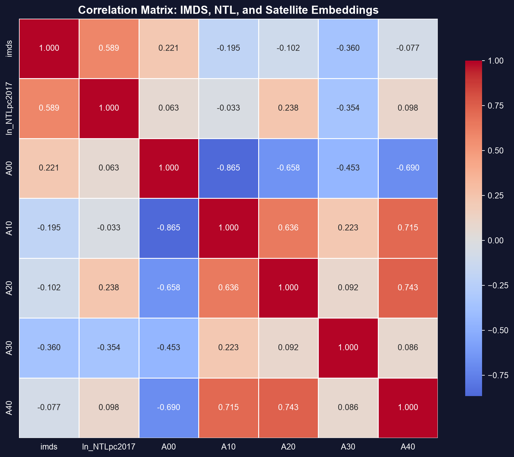
#### Task 2: Correlation Analysis (Guided)
**Objective**: Compute and visualize the correlation structure among all predictors and the outcome variable.
**Instructions**:
1. Compute the correlation matrix for `imds`, `ln_NTLpc2017`, and all five embedding variables
2. Display the correlation matrix as a heatmap
3. Identify: Which embeddings correlate most strongly with `imds`?
4. Identify: Do the embeddings correlate with each other (potential multicollinearity)?
5. Do the embeddings correlate with NTL, or do they capture different information?
**Apply what you learned in section 10.3**: Use `seaborn.heatmap()` with annotated correlation values.
```{python}
# Your code here: Correlation analysis of satellite predictors
#
# Step 1: Compute correlation matrix
corr_vars = ['imds', 'ln_NTLpc2017', 'A00', 'A10', 'A20', 'A30', 'A40']
corr_sat = bol_sat[corr_vars].dropna().corr()

# CORRELATION MATRIX: DEVELOPMENT AND SATELLITE PREDICTORS
print(corr_sat.round(3))

# Step 2: Visualize as heatmap
fig, ax = plt.subplots(figsize=(10, 8))
sns.heatmap(corr_sat, annot=True, fmt='.3f', cmap='coolwarm', center=0,
            square=True, linewidths=1, cbar_kws={"shrink": 0.8})
ax.set_title('Correlation Matrix: IMDS, NTL, and Satellite Embeddings',
             fontsize=14, fontweight='bold')
plt.tight_layout()
plt.show()

# Step 3: Highlight strongest correlations with IMDS
# Correlations with IMDS
imds_corr = corr_sat['imds'].drop('imds').sort_values(key=abs, ascending=False)
for var, r in imds_corr.items():
    print(f"  {var:16s}  r = {r:+.3f}")
```
> **Key Concept 10.11: High-Dimensional Satellite Features**
>
> Satellite embeddings are **64 abstract features** extracted by deep learning models (convolutional neural networks) from daytime satellite imagery. Unlike handcrafted variables (e.g., NDVI for vegetation), each embedding dimension captures complex visual patterns — road density, building structures, agricultural layouts — learned automatically from the data. These features are not directly interpretable (dimension A00 doesn't have a specific meaning), but they collectively encode rich information about a municipality's physical landscape.
#### Task 3: Multiple Regression (Semi-guided)
**Objective**: Estimate a multiple regression model with NTL and satellite embeddings as predictors.
**Instructions**:
1. Estimate the full model: `imds ~ ln_NTLpc2017 + A00 + A10 + A20 + A30 + A40`
2. Display the regression summary
3. Compare $R^2$ with the bivariate NTL-only model from Chapter 1
4. Interpret: How much does adding embeddings improve explanatory power?
5. Which embedding coefficients are statistically significant?
**Apply what you learned in section 10.4**: Use `pf.feols()` from pyfixest and interpret partial effects.
```{python}
# Your code here: Multiple regression with satellite predictors
#
# Step 1: Prepare data (drop missing values)
reg_data = bol_sat[['imds', 'ln_NTLpc2017', 'A00', 'A10', 'A20', 'A30', 'A40']].dropna()
print(f"Regression sample: {len(reg_data)} municipalities (complete cases)")

# Step 2: Bivariate model (NTL only — baseline from Chapter 1)
model_ntl = pf.feols('imds ~ ln_NTLpc2017', data=reg_data)
# MODEL 1: BIVARIATE — imds ~ ln_NTLpc2017
model_ntl.summary()

# Step 3: Multiple regression (NTL + all 5 embeddings)
model_full_sat = pf.feols('imds ~ ln_NTLpc2017 + A00 + A10 + A20 + A30 + A40', data=reg_data)
# MODEL 2: MULTIPLE — imds ~ ln_NTLpc2017 + A00 + A10 + A20 + A30 + A40
model_full_sat.summary()

# Step 4: Compare R-squared
# R-SQUARED COMPARISON
print(f"NTL only:           R² = {model_ntl._r2:.4f}")
print(f"NTL + 5 embeddings: R² = {model_full_sat._r2:.4f}")
print(f"Improvement:        ΔR² = {model_full_sat._r2 - model_ntl._r2:.4f}")
```
#### Task 4: Partial Effects via FWL (Semi-guided)
**Objective**: Demonstrate the Frisch-Waugh-Lovell theorem by showing that the NTL coefficient in the multiple regression equals the coefficient from regressing residualized IMDS on residualized NTL.
**Instructions**:
1. Regress `imds` on all embedding variables (`A00`, `A10`, `A20`, `A30`, `A40`), save residuals $e_y$
2. Regress `ln_NTLpc2017` on all embedding variables, save residuals $e_x$
3. Regress $e_y$ on $e_x$ (bivariate regression of residuals)
4. Verify that the coefficient matches the NTL coefficient from the full multiple regression
**Apply what you learned in section 10.5**: This demonstrates that the partial effect of NTL is computed from the variation in NTL that is *independent* of the satellite embeddings.
```{python}
# Your code here: FWL theorem demonstration
#
# Step 1: Regress imds on embeddings only, save residuals e_y
model_y_on_emb = pf.feols('imds ~ A00 + A10 + A20 + A30 + A40', data=reg_data)
e_y = model_y_on_emb._u_hat

# Step 2: Regress ln_NTLpc2017 on embeddings only, save residuals e_x
model_x_on_emb = pf.feols('ln_NTLpc2017 ~ A00 + A10 + A20 + A30 + A40', data=reg_data)
e_x = model_x_on_emb._u_hat

# Step 3: Regress e_y on e_x
fwl_data = pd.DataFrame({'e_y': e_y, 'e_x': e_x})
model_fwl = pf.feols('e_y ~ e_x', data=fwl_data)

# Step 4: Compare coefficients
# FWL THEOREM DEMONSTRATION
print(f"NTL coefficient from FULL multiple regression:  {model_full_sat.coef()['ln_NTLpc2017']:.10f}")
print(f"Coefficient from FWL residual regression:       {model_fwl.coef()['e_x']:.10f}")
print(f"Difference (numerical precision):                {abs(model_full_sat.coef()['ln_NTLpc2017'] - model_fwl.coef()['e_x']):.15f}")
# The coefficients are identical — confirming the FWL theorem
```
#### Task 5: Model Comparison (Independent)
**Objective**: Compare multiple model specifications using fit statistics and information criteria.
**Your tasks**:
1. Estimate three models:
- **Model 1**: `imds ~ ln_NTLpc2017` (NTL only)
- **Model 2**: `imds ~ ln_NTLpc2017 + A00 + A10` (NTL + 2 embeddings)
- **Model 3**: `imds ~ ln_NTLpc2017 + A00 + A10 + A20 + A30 + A40` (NTL + 5 embeddings)
2. Create a comparison table reporting $R^2$, adjusted $R^2$, AIC, and BIC for each model
3. Compute fit statistics from `model._r2` and `model._adj_r2`; pyfixest has no `._aic`/`._bic`, so compute AIC/BIC from the residuals as `n*np.log(rss/n) + n*(1+np.log(2*np.pi)) + 2*k` and `... + k*np.log(n)` (with `rss = np.sum(model._u_hat**2)`, `n = int(model._N)`, `k = len(model.coef())`)
4. Which model is "best" by each criterion?
5. Does the parsimony principle favor fewer or more embedding variables?
*Hint: Use `pd.DataFrame()` to create a clean comparison table.*
```{python}
# Your code here: Model comparison
#
# Step 1: Estimate three models
# model_1 = pf.feols('imds ~ ln_NTLpc2017', data=reg_data)
# model_2 = pf.feols('imds ~ ln_NTLpc2017 + A00 + A10', data=reg_data)
# model_3 = pf.feols('imds ~ ln_NTLpc2017 + A00 + A10 + A20 + A30 + A40', data=reg_data)
#
# Step 2: Create comparison table
# comparison = pd.DataFrame({
#     'Model': ['NTL only', 'NTL + 2 embeddings', 'NTL + 5 embeddings'],
#     'R²': [model_1._r2, model_2._r2, model_3._r2],
#     'Adj R²': [model_1._adj_r2, model_2._adj_r2, model_3._adj_r2],
#     # pyfixest has no ._aic/._bic; compute them (Stata convention) from each model's RSS:
#     #   def stata_ic(m):
#     #       n_m, k_m = int(m._N), len(m.coef()); rss_m = np.sum(m._u_hat**2); c = n_m*(1+np.log(2*np.pi))
#     #       return (n_m*np.log(rss_m/n_m)+c+2*k_m, n_m*np.log(rss_m/n_m)+c+k_m*np.log(n_m))
#     'AIC': [stata_ic(model_1)[0], stata_ic(model_2)[0], stata_ic(model_3)[0]],
#     'BIC': [stata_ic(model_1)[1], stata_ic(model_2)[1], stata_ic(model_3)[1]],
#     'N': [len(reg_data)] * 3
# })
# print(comparison.to_string(index=False))
#
# Step 3: Interpret — which model is preferred by each criterion?
```
> **Key Concept 10.12: Incremental Predictive Power**
>
> When adding predictors to a regression model, $R^2$ can only increase or stay the same — it never decreases. This makes $R^2$ misleading for model comparison when models have different numbers of predictors. **Adjusted $R^2$** penalizes for additional variables, while **AIC** and **BIC** balance fit against complexity. In the satellite prediction context, adding all 64 embeddings would maximize $R^2$ but might overfit; information criteria help identify the most parsimonious model.
#### Task 6: Policy Brief on Satellite Prediction (Independent)
**Objective**: Write a 200-300 word policy brief summarizing the value of satellite embeddings for development prediction.
**Your brief should address:**
1. **Improvement**: How much does adding satellite embeddings improve development prediction compared to NTL alone?
2. **Complexity trade-off**: Is the improvement worth the added model complexity? What do adjusted $R^2$, AIC, and BIC suggest?
3. **Partial effects**: After controlling for embeddings, does NTL remain a significant predictor? What does the FWL theorem reveal about NTL's independent contribution?
4. **SDG monitoring implications**: How could multi-source satellite data enhance SDG monitoring in data-scarce countries like Bolivia?
5. **Limitations**: What can satellite data *not* capture about development? What are the risks of relying on abstract embedding features for policy decisions?
**Connection to Research**: The DS4Bolivia project uses all 64 embedding dimensions plus machine learning methods (Random Forest, XGBoost) to predict SDG indicators, achieving meaningful predictive accuracy. Your multiple regression analysis provides a transparent, interpretable baseline for comparison.
```{python}
# Your code here: Additional analysis for the policy brief
#
# You might want to:
# 1. Create a summary table of key results across models
# 2. Generate a visualization comparing model fit
# 3. Calculate the percentage improvement in R² from adding embeddings
# 4. Discuss which embeddings contribute most to prediction
#
# Example:
# print("KEY RESULTS FOR POLICY BRIEF")
# print(f"NTL-only R²:          {model_1._r2:.4f}")
# print(f"NTL + 5 embed R²:     {model_3._r2:.4f}")
# print(f"R² improvement:       {(model_3._r2 - model_1._r2) / model_1._r2 * 100:.1f}%")
# print(f"NTL coef (bivariate): {model_1.coef()['ln_NTLpc2017']:.4f}")
# print(f"NTL coef (multiple):  {model_3.coef()['ln_NTLpc2017']:.4f}")
```
#### What You've Learned from This Case Study
Through this analysis of multiple satellite predictors of Bolivian municipal development, you've applied the full Chapter 10 toolkit to a cutting-edge research application:
- **Correlation analysis**: Explored the correlation structure among NTL, satellite embeddings, and development outcomes
- **Multiple regression**: Estimated models with multiple satellite predictors and interpreted partial effects
- **FWL theorem**: Demonstrated that the partial effect of NTL equals the coefficient from regressing residualized IMDS on residualized NTL
- **Model comparison**: Evaluated competing specifications using $R^2$, adjusted $R^2$, AIC, and BIC
- **Critical assessment**: Weighed the predictive gains from additional satellite features against model complexity
**Connection to upcoming chapters**: In Chapter 11, we'll test whether the satellite embeddings are *statistically* significant using F-tests for joint significance. In Chapter 12, we'll address robust inference and prediction intervals.
**This dataset returns throughout the textbook**: Each subsequent chapter applies its specific econometric tools to the DS4Bolivia data, building progressively toward a comprehensive satellite-based development prediction framework.
---
**Well done!** You've now analyzed how multiple satellite data sources can predict development outcomes, moving from simple bivariate regression (Chapter 1) to the richer multiple regression framework of Chapter 10.