The question

Act I · The tension

Economists can’t run experiments on the economy

We can’t randomly assign people different incomes, or give one city a tax cut and another none.

So how do we measure how one economic variable moves with another? Regression — the primary tool of econometrics — turns a cloud of observed data into a line we can read.

Unlike a lab science, economics works mostly with observational data. Regression is how we quantify relationships from data we did not get to control.

Where we’re going

• What regression is — and why it’s econometrics’ main tool
• Load & explore economic data with pandas
• Visualize the relationship with a scatter plot
• Fit a simple regression by OLS with pyfixest
• Interpret the slope, intercept, and \(R^2\) — in economic terms

Six ideas anchor this chapter

• Regression — a statistical line of best fit through the data
• Y vs X — the outcome we explain (\(Y\)) and the explainer (\(X\))
• Intercept \(\beta_0\) · slope \(\beta_1\) — where the line starts, and how steep it is
• OLS — picks the line that minimizes the sum of squared residuals
• \(R^2\) — the share of variation in \(Y\) the line explains (0 to 1)
• Association \(\neq\) causation — regression measures how \(Y\) and \(X\) move together, not cause

The slope is almost always the number you actually care about.

From data to a fitted line

Act II · The investigation

Our question: do bigger houses sell for more?

29 house sales in Davis, California (1999). Two columns carry the story: price and size.

\[\text{price} = \beta_0 + \beta_1 \cdot \text{size} + \varepsilon\]

We want \(\beta_1\) — the predicted change in price per extra square foot. OLS chooses \(\beta_0, \beta_1\) to make the squared gaps between the dots and the line as small as possible.

Step 1 — load and explore the data with pandas

import pandas as pd                          # pandas → load & handle tabular data

# dataset: 29 house sales in Davis, CA, 1999 (price, size, bedrooms, …)
url = "https://raw.githubusercontent.com/quarcs-lab/data-open/master/AED/AED_HOUSE.DTA"
data = pd.read_stata(url)                    # read the Stata .dta into a DataFrame

data.head()                                  # peek at the first few rows
data.describe().round(2)                     # summary stats: mean, std, min, max, quartiles

↗ Try it in Colab

Mean price ≈ $253,910, mean size ≈ 1,883 sq ft; price ranges $204k–$375k. Always describe before you model — the scale and spread make the regression interpretable later.

Step 2 — always visualize before you model

import pandas as pd                          # tabular data
import matplotlib.pyplot as plt               # plotting

url = "https://raw.githubusercontent.com/quarcs-lab/data-open/master/AED/AED_HOUSE.DTA"
data = pd.read_stata(url)                    # load the 29 Davis, CA house sales

fig, ax = plt.subplots(figsize=(10, 6))      # one figure + axes
ax.scatter(data["size"], data["price"],      # x = size, y = price
           s=80, alpha=0.7, color="#22d3ee") # marker size, transparency, colour
plt.show()                                   # render the scatter plot

↗ Try it in Colab

Price rises with size — the relationship is real but loose

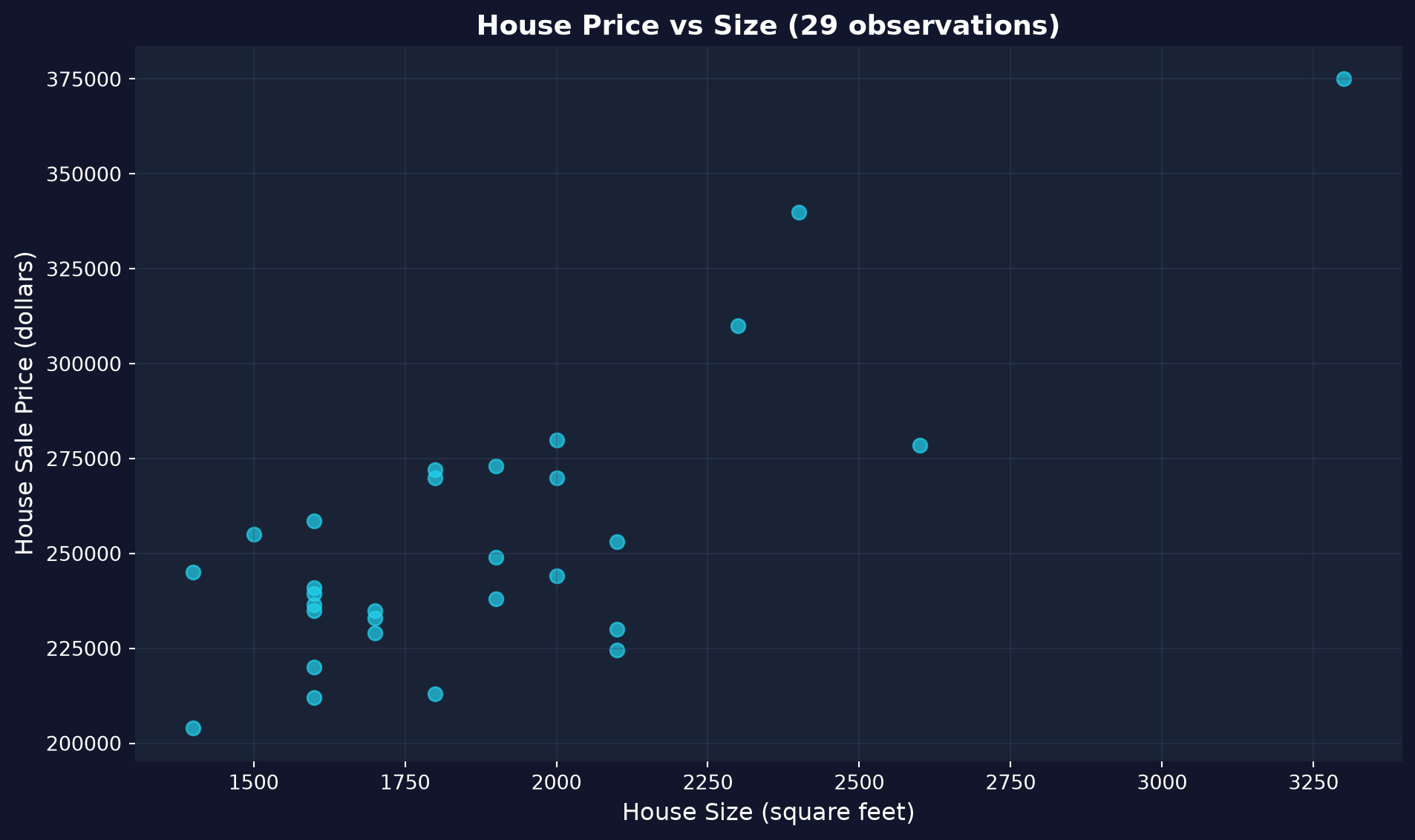
Each dot is a house. The upward drift is the relationship; the vertical scatter is everything size doesn’t explain.

A scatter plot is the honest first look — it shows direction and spread before any model.

Step 3 — fit the regression by OLS with pyfixest

!pip install -q pyfixest                     # install pyfixest in Colab (-q = quiet; not preinstalled)

import pandas as pd                          # tabular data
import pyfixest as pf                         # pyfixest → OLS regression, R-style formulas

url = "https://raw.githubusercontent.com/quarcs-lab/data-open/master/AED/AED_HOUSE.DTA"
data = pd.read_stata(url)                    # load the 29 Davis, CA house sales

fit = pf.feols("price ~ size", data=data)    # OLS: regress price on size (intercept auto-added)
fit.summary()                                # β0, β1, SEs, t, p, R²

↗ Try it in Colab

pyfixest.feols is the project’s estimation tool — the same y ~ x formula syntax as R’s fixest. One line fits the model; summary() prints the full table.

OLS draws the line: price = 115,017 + 73.77 × size

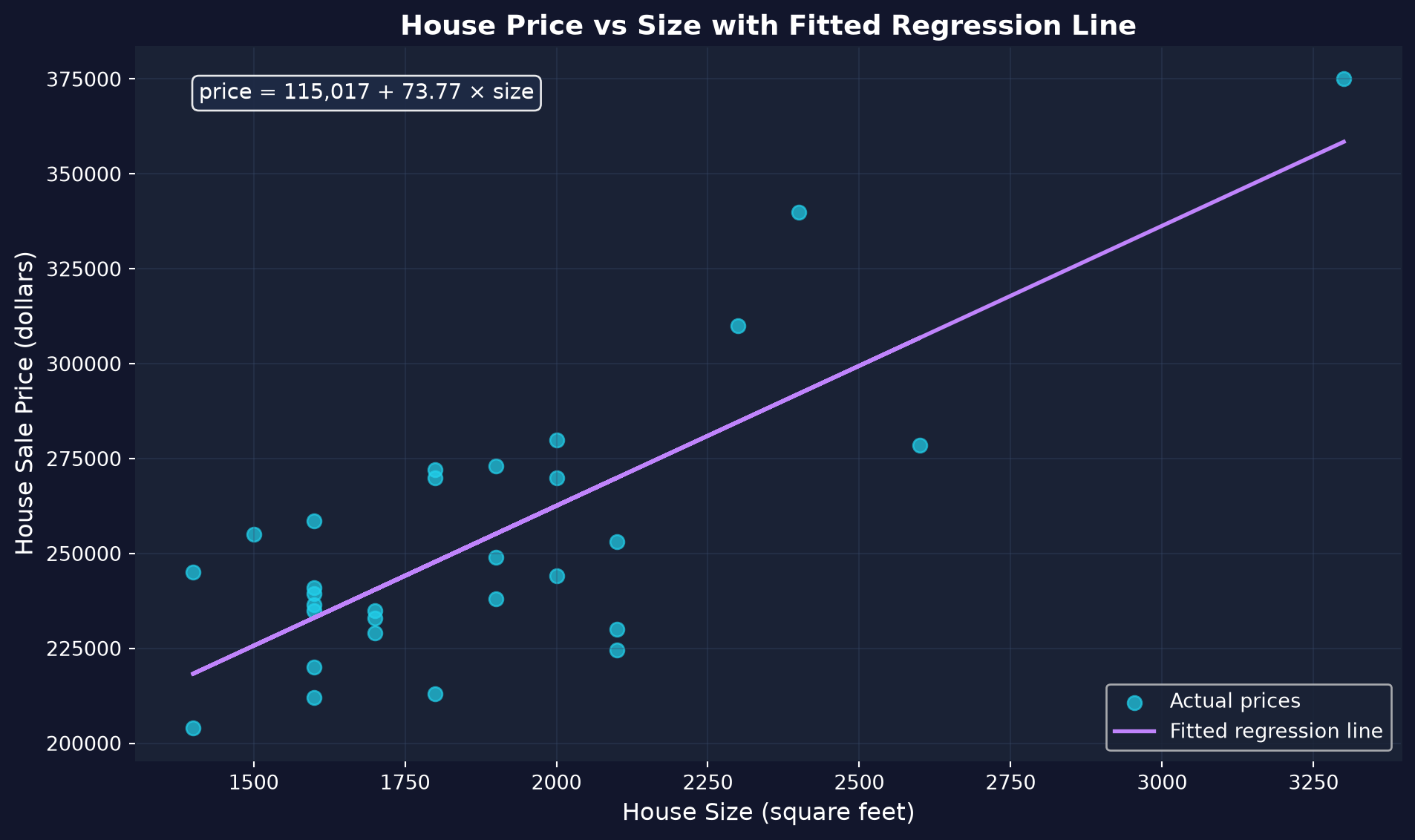
The fitted line through the cloud, with its equation.

Slope \(\beta_1 = \$73.77\)/sq ft · intercept \(\beta_0 = \$115{,}017\) · \(R^2 = 0.62\).

Reading the three numbers

• Slope \(\beta_1 = \$73.77\) — each extra square foot is associated with about $74 more in price (≈ $7,400 per 100 sq ft).
• Intercept \(\beta_0 = \$115{,}017\) — just where the line crosses \(x=0\); a 0-sq-ft house isn’t meaningful, so don’t over-read it.
• \(R^2 = 0.62\) — size alone explains about 62% of the price variation; the other 38% is location, condition, age, …

Report magnitude, not just significance: $74 per square foot is the economically meaningful finding.

Reading it right

Act III · The resolution

The tempting mistake — and the correction

Objection. “Each square foot adds $74 — so extending my house 100 sq ft adds $7,400.”

Response. Association is not causation. Bigger houses may also be better-located and better-renovated — the slope credits size for quality’s effect too. Like ice-cream sales and drownings: both rise in summer, but one doesn’t cause the other.

Regression shows how \(Y\) and \(X\) move together; a causal reading needs a design that rules out the alternatives.

What to carry forward

• Regression is econometrics’ primary tool: it quantifies how \(Y\) varies with \(X\).
• The simple model is \(y = \beta_0 + \beta_1 x + \varepsilon\); OLS minimizes squared residuals.
• The slope measures association; \(R^2\) measures fit — neither proves causation.
• The Python workflow is load → explore → visualize → model → interpret (pandas, matplotlib, pyfixest).
• Don’t extrapolate beyond the data, and don’t assume the sample generalizes.

Fit the line, read the slope — then ask whether it’s really a cause.