The question

Act I · The tension

One sample mean is just one draw

You survey 30 people and get an average income of $52,000. Someone else surveys a different 30 and gets $48,000. Who is right?

Both. Each $\bar{x}$ is one realization of a random variable $\bar{X}$ that changes from sample to sample. This chapter asks: what does the distribution of $\bar{X}$ look like — and how do we use it?

Where we’re going

$\bar{X}$ is a random variable — not a fixed number
Its mean and variance: $E[\bar{X}] = \mu$ and $\operatorname{Var}[\bar{X}] = \sigma^2/n$
Its sampling distribution — seen through a coin-toss experiment
The Central Limit Theorem: $\bar{X}$ is approximately normal, even from skewed data
The standard error $se(\bar{X}) = s/\sqrt{n}$ — and why bigger $n$ means sharper estimates

Six ideas anchor this chapter

Parameter vs. statistic — $\mu$ is fixed and unknown; $\bar{x}$ is computed and varies
Estimator — a rule ($\bar{X} = \tfrac{1}{n}\sum X_i$); an estimate is one number it returns
Unbiasedness — $E[\bar{X}] = \mu$: no systematic over- or under-shoot
Efficiency — among unbiased estimators, $\bar{X}$ has the smallest bounce
Consistency — $\operatorname{Var}[\bar{X}] = \sigma^2/n \to 0$, so $\bar{X} \to \mu$ as $n$ grows
Law of Large Numbers — the formal guarantee behind that convergence

The number you compute is random; its distribution is what inference is built on.

From one sample to a distribution

Act II · The investigation

The experiment: 400 samples of 30 coin tosses

A fair coin has $\mu = 0.5$ and $\sigma^2 = 0.25$. Toss it 30 times, record the fraction of heads — that’s one $\bar{x}$. Do it 400 times and you can watch the sampling distribution emerge.

\[\bar{X} = \frac{1}{n}\sum_{i=1}^{n} X_i, \qquad E[\bar{X}] = \mu, \qquad \operatorname{Var}[\bar{X}] = \frac{\sigma^2}{n}\]

The textbook pre-computed the 400 means for us — let’s load and summarize them first.

Step 1 — load and summarize the 400 sample means with pandas

import pandas as pd                          # pandas → load & handle tabular data
import numpy as np                           # numpy → sqrt and array math

url = "https://raw.githubusercontent.com/quarcs-lab/data-open/master/AED/AED_COINTOSSMEANS.DTA"
data = pd.read_stata(url)                    # 400 sample means, each from n = 30 tosses
xbar = data["xbar"]                          # the column of 400 sample means

print(xbar.mean())                           # empirical E[X̄]  → 0.5004
print(xbar.std())                            # empirical SD     → 0.0887

print(np.sqrt(0.25 / 30))                    # theoretical σ/√n → 0.0913
data.describe().round(4)                      # full summary of the 400 means

↗ Try it in Colab

The 400 means pile up in a bell around 0.5

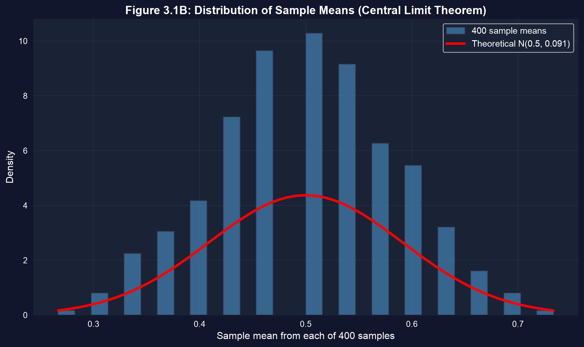
Each bar counts how often a sample mean landed in that range; the curve is the theoretical $N(\mu,\,\sigma^2/n)$.

The histogram of sample means is the sampling distribution — centered at $\mu$, spread $\sigma/\sqrt{n}$.

Precision is a formula: $sd(\bar{X}) = \sigma/\sqrt{n}$

Larger samples don’t shift the center — they shrink the spread. The catch: it shrinks with $\sqrt{n}$, not $n$.

$n$	$\sigma/\sqrt{n}$
10	0.158
30	0.091
100	0.050
400	0.025
1000	0.016

To halve the standard error you must quadruple the sample size — precision is expensive.

Step 2 — reproduce the distribution with a Monte Carlo simulation

import numpy as np                           # numpy → random draws + arrays

np.random.seed(10101)                        # fix the seed → reproducible result
means = np.zeros(400)                        # container for 400 sample means
for i in range(400):                         # repeat the experiment 400 times
    sample = np.random.binomial(1, 0.5, 30)  # 30 fair coin tosses (each 0 or 1)
    means[i] = sample.mean()                 # store this sample's mean X̄

print(means.mean())                          # ≈ 0.50   → unbiased
print(means.std())                           # ≈ 0.091  → matches σ/√n

↗ Try it in Colab

The Central Limit Theorem: skewed data, normal mean

1880 U.S. Census ages are heavily right-skewed ($\mu = 24.13$, $\sigma = 18.61$). Yet the means of 100 samples of $n = 25$ trace a familiar bell.

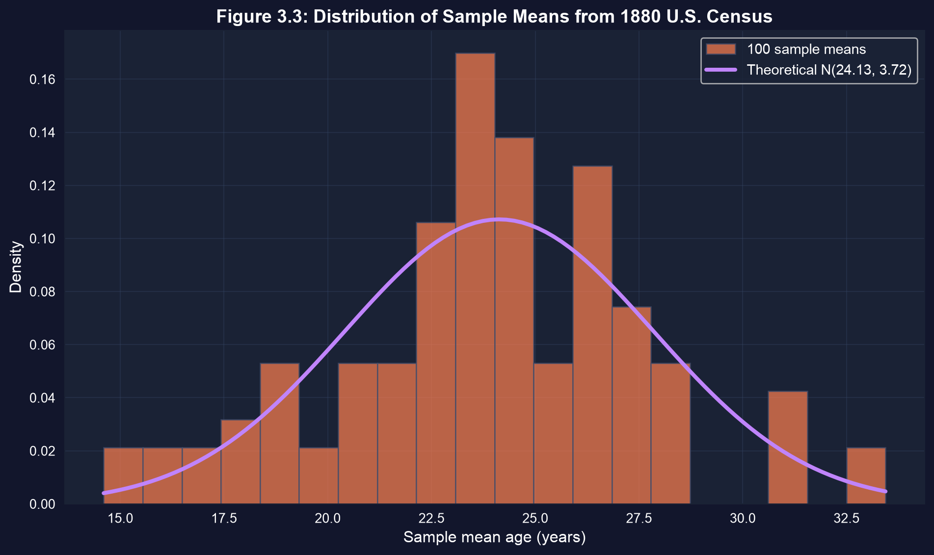
100 sample means of 1880 census ages — a bell curve rising from a skewed population.

The CLT: average enough draws and $\bar{X}$ goes normal — whatever the population’s shape.

Step 3 — visualize a sampling distribution with its theoretical normal

import numpy as np, pandas as pd             # arrays + data
import matplotlib.pyplot as plt               # plotting
from scipy.stats import norm                  # scipy → the normal pdf for the overlay

url = "https://raw.githubusercontent.com/quarcs-lab/data-open/master/AED/AED_COINTOSSMEANS.DTA"
xbar = pd.read_stata(url)["xbar"]            # the 400 coin-toss sample means

fig, ax = plt.subplots(figsize=(10, 6))      # one figure + axes
ax.hist(xbar, bins=20, density=True,         # empirical sampling distribution
        color="#008CB7", alpha=0.75)         # (density so it compares to a pdf)
grid = np.linspace(xbar.min(), xbar.max(), 200)
ax.plot(grid, norm.pdf(grid, 0.5, np.sqrt(0.25 / 30)),  # theoretical N(μ, σ²/n)
        color="#C21E72", lw=3)               # DataPink curve on top
plt.show()                                   # render histogram + normal overlay

↗ Try it in Colab

Three marks of a good estimator — and $\bar{X}$ earns all three

Unbiased — across 400 coin samples the means average 0.5004 vs. true $\mu = 0.5$.
Efficient — its SD 0.0887 sits right at the theoretical floor $\sigma/\sqrt{n} = 0.0913$; no rival unbiased rule bounces less.
Consistent — $\operatorname{Var}[\bar{X}] = \sigma^2/n \to 0$: for census ages the SD of $\bar{X}$ falls from 3.72 at $n=25$ to 0.26 at $n=5{,}000$.

Unbiased, efficient, consistent — this is why the sample mean is the workhorse estimator.

Reading it right

Act III · The resolution

The catch — the sample must be representative

Objection. “More data always gets me closer to the truth.”

Response. Only under simple random sampling. Oversample one group — say 70% women when the population is 50/50 — and the plain mean is biased, no matter how large $n$ is. The fix is a weighted mean with inverse-probability weights $w_i = 1/\pi_i$, which restores the true population average.

Consistency assumes a representative sample; a biased design converges to the wrong number.

What to carry forward

A sample mean $\bar{x}$ is one draw of the random variable $\bar{X}$.
$E[\bar{X}] = \mu$ (unbiased) and $\operatorname{Var}[\bar{X}] = \sigma^2/n$ (precision grows with $n$).
The standard error $se(\bar{X}) = s/\sqrt{n}$ — halving it costs 4× the data.
The CLT makes $\bar{X}$ approximately normal even when the population is not.
All of it assumes a representative sample; otherwise, weight to correct the design.

Compute the mean — then remember it’s a draw from a distribution.

The question

One sample mean is just one draw

Where we’re going

Six ideas anchor this chapter

From one sample to a distribution

The experiment: 400 samples of 30 coin tosses

Step 1 — load and summarize the 400 sample means with pandas

The 400 means pile up in a bell around 0.5

Precision is a formula: \(sd(\bar{X}) = \sigma/\sqrt{n}\)

Step 2 — reproduce the distribution with a Monte Carlo simulation

The Central Limit Theorem: skewed data, normal mean

Step 3 — visualize a sampling distribution with its theoretical normal

Three marks of a good estimator — and \(\bar{X}\) earns all three

Reading it right

The catch — the sample must be representative

What to carry forward

Compute the mean — then remember it’s a draw from a distribution.