One sample, a whole population

Act I · The tension

This is the chapter on which every later chapter rests. Every regression table in the book reports a standard error, a t statistic, a p-value and a confidence interval, and all four are introduced here for the simplest possible estimator: the sample mean. If students master the logic for one mean, the regression chapters only change the estimator, not the reasoning.

We measure a sample, but we care about the population

We surveyed 171 women aged 30 who work full time and found mean earnings of $41,413. We do not care about these 171 people as such. We care about all 30-year-old women working full time in the U.S. in 2010.

The sample mean \(\bar{x}\) is our best guess of the population mean \(\mu\), but it is only one draw: another sample of 171 would give a different number. Statistical inference turns that single number into a statement with quantified uncertainty, either a range (a confidence interval) or a verdict on a claim (a hypothesis test).

The whole chapter answers one question: how far from \(\mu\) could \(\bar{x}\) plausibly be?

Inference is the bridge from the sample we have to the population we want to describe. Stress that the population mean is a fixed, unknown number; what is random is the sample, and therefore the sample mean and every interval built from it.

Eleven stops — click any row to jump to it

Stop	Question	Tool	Headline result
4.1	How precise is one sample mean?	standard error \(s/\sqrt{n}\)	$41,413, SE $1,952
4.2	Which ruler do we measure with?	\(t\) distribution	\(t_{170,\,0.025} = 1.974\)
4.3	What values of \(\mu\) are plausible?	confidence interval	95% CI [$37,559, $45,266]
4.4	Is \(\mu = \$40{,}000\) credible?	two-sided \(t\) test, power	\(t = 0.72\), \(p = 0.470\)
4.5	Gas, male earnings, GDP growth	three tests	only gas rejects (\(t = -5.26\))
4.6	Does \(\mu\) exceed $40,000?	one-sided test	\(p = 0.235\)
4.7	Is the race tied?	proportions, \(z\) test	52.1%, \(p = 0.199\)
CS 1	Has world productivity changed?	CIs, Welch & paired tests	paired \(t = 10.90\)
CS 2	Is Bolivia’s development equal?	CIs, one- & two-sample tests	Tarija − Pando = 14.7 points
Synthesis	What did all the tests say?	one ruler, one checklist	—

Sections 4.1–4.7 follow the chapter. The two case studies run every one of their six tasks with real output; results the chapter does not print are labelled “computed for these slides”. Press M for the menu or O for the overview grid; the stop labels are links.

One formula carries the whole chapter

\[t \;=\; \frac{\text{estimate} \;-\; \text{hypothesized value}}{\text{standard error}} \qquad\qquad \text{CI} \;=\; \text{estimate} \;\pm\; \text{critical value} \times \text{standard error}\]

• The estimate here is \(\bar{x}\) (or \(\hat{p}\) for a proportion); in Chapter 7 it becomes a regression slope \(b_2\)
• The standard error measures how much the estimate would vary across repeated samples
• The critical value comes from the \(t\) distribution (or the normal for proportions)

Learn this pair of formulas once and you can read every inference table in the book.

Key Takeaway 9 of the chapter: the methods generalize to other parameters. Point forward explicitly: in Chapter 7 the same t = (b − β*)/se(b) and b ± t × se(b) appear in every regression output.

Seven ideas anchor this chapter

• \(H_0\) vs \(H_a\): the default claim we test, and the alternative we accept if it falls
• Test statistic \(t\): how many standard errors the estimate sits from the value in \(H_0\)
• \(p\)-value: the probability of data at least this extreme if \(H_0\) were true
• Significance level \(\alpha\): the false-alarm rate we accept, usually \(0.05\)
• Critical value: the cutoff on \(t\) that bounds the rejection region
• Type I / Type II error: a false alarm vs a missed effect; power \(= 1-\beta\)
• Confidence interval: the range of \(\mu\) values a two-sided test would not reject

A test never proves \(H_0\). It only asks whether the data can reject it.

These are the chapter’s Key Concepts glossary. Spend time on the p-value definition: it is a probability about the data computed under H0, never the probability that H0 is true.

A thread through every slide: three questions for any test

Question	Answered by	Fails when…
Is it real?	\(t\), \(p\)-value, CI	the gap is small relative to the SE
Does it matter?	the size of the gap, in units people care about	a precise estimate of a trivial gap
Could we even tell?	power, the width of the CI	a real gap hidden by a large SE

Every example in this deck gets all three questions. Statistical significance answers only the first.

This is the recurring thread of the deck. Gas prices (4.5) are real and matter; female earnings vs $40,000 (4.4) might matter but we could not tell; Bolivia’s mean IMDS vs 50 (CS2) is real but barely matters. The synthesis slide at the end puts every test on one ruler.

Act II · From one sample to the population

Sections 4.1–4.7 · estimate, interval, test

Seven sections, each with the same arc: question → method → code → output → interpretation → caveats. The female earnings sample carries sections 4.1–4.4 and 4.6; section 4.5 adds three new datasets; 4.7 switches to yes/no data.

Section 4.1 · How precise is one sample mean?

Sample mean · standard deviation · standard error

Section 4.1: the motivating example. Tools: the sample mean, the sample standard deviation, and the standard error.

The question: what do 30-year-old women earn?

Data. AED_EARNINGS.DTA: 171 women aged 30 working full time in the U.S. in 2010, annual earnings in dollars.

Symbol	Name	Measures
\(\bar{x}\)	sample mean	our point estimate of the population mean \(\mu\)
\(s\)	sample standard deviation	how much individual earnings vary
\(\text{se}(\bar{x}) = s/\sqrt{n}\)	standard error	how much the sample mean would vary across samples

Two different spreads: \(s\) describes people; the standard error describes our estimate.

The data are a sample from a much larger population. The chapter’s Key Concept 4.1: the standard error measures the precision of x̄ as an estimate of μ. Students regularly confuse s and se; this table is worth pausing on.

Earnings are right-skewed: a few high earners pull the mean up

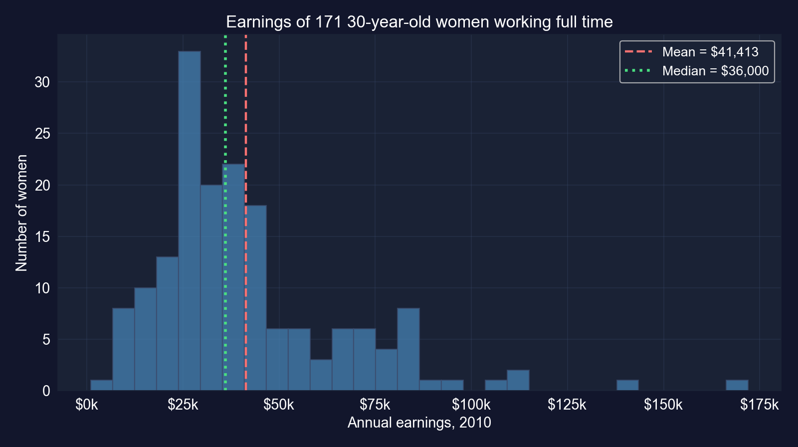
Earnings of the 171 women. The mean ($41,413) sits above the median ($36,000).

64% of the women earn less than the mean. Inference here is about the mean, which is not the typical earner.

Figure computed for these slides from the chapter’s data. Earnings run from $1,050 to $172,000; skewness 1.71. With n = 171 the central limit theorem makes the sampling distribution of the mean close to normal even though earnings are skewed, so t-based inference is still reasonable. With very small samples from a skewed population it would not be.

Code: load the data and compute the standard error

import numpy as np                          # square roots
import pandas as pd                         # tabular data
from scipy import stats                     # t and normal distributions (used later)
url = "https://raw.githubusercontent.com/quarcs-lab/data-open/master/AED/AED_EARNINGS.DTA"
data_earnings = pd.read_stata(url)          # 171 women aged 30, full-time, 2010
earnings = data_earnings["earnings"]        # annual earnings in dollars
n = len(earnings)                           # sample size
mean_earnings = earnings.mean()             # sample mean x-bar
std_earnings = earnings.std(ddof=1)         # sample std dev s (divides by n - 1)
se_earnings = std_earnings / np.sqrt(n)     # standard error = s / sqrt(n)
print(f"n = {n}")                           # 171
print(f"Mean: ${mean_earnings:,.2f}")       # point estimate of mu
print(f"Std dev: ${std_earnings:,.2f}")     # spread across women
print(f"Std error: ${se_earnings:,.2f}")    # spread of x-bar across samples

↗ Try it in Colab

Self-contained: paste into an empty Colab cell. ddof=1 gives the sample standard deviation, dividing by n − 1 rather than n. Everything in sections 4.2–4.4 and 4.6 reuses these four numbers.

Output: a precise estimate from a noisy sample

Statistic	Value
\(n\)	171
Mean \(\bar{x}\)	$41,412.69
Median	$36,000.00
Std. deviation \(s\)	$25,527.05
Std. error \(s/\sqrt{n}\)	$1,952.10

\(\text{se} = 25{,}527.05/\sqrt{171} = 1{,}952.10\)

How the SE scales with \(n\) (same \(s\)):

Sample size	SE
\(n = 43\) (¼ as many)	$3,893
\(n = 171\) (ours)	$1,952
\(n = 684\) (4× as many)	$976

Individual earnings vary by about $25,500, but the average of 171 of them varies by only about $1,950.

The SE is 13 times smaller than s because √171 ≈ 13.1. With 43 women the SE would roughly double, to $3,893: not exactly 2 × 1,952 = 3,904, because 43 is slightly more than 171/4. In general, quartering the sample doubles the SE and quadrupling it halves the SE.

Reading the standard error

• Repeated-sampling meaning: if we drew many samples of 171 women, their means would typically differ from \(\mu\) by about $1,950
• Precision relative to the mean: $1,952 is under 5% of $41,413, so the estimate is reasonably precise
• Square-root law: precision grows with \(\sqrt{n}\), so halving the SE costs four times the data

Key Concept 4.1: the standard error is the single number behind every interval and test that follows.

The square-root law is why surveys get expensive: going from ±$3,900 to ±$1,950 needs 4× the sample, and to ±$975 needs 16×.

What the standard error assumes

It requires

• a random sample: each woman is an independent draw from the population
• the formula \(s/\sqrt{n}\) is built on independence

It does not capture

• non-sampling error: misreported earnings, non-response
• dependence: clustered or time-series data need other SEs (Ch. 7, 12, 17)

The SE measures sampling noise only, and only under independence. GDP growth in 4.5 will show what happens when independence fails.

Standard caveat. The formula is derived for independent draws. Survey data with clusters, or time series where this quarter resembles the last, violate it, and the s/√n formula then understates the real uncertainty.

Section 4.2 · Why a \(t\) ruler, not a normal one?

\(t\) statistic · degrees of freedom · fat tails

Section 4.2: the t statistic and the t distribution. Tools: standardizing the sample mean, degrees of freedom, critical values.

The \(t\) statistic standardizes the sample mean

\[t = \frac{\bar{x} - \mu}{\text{se}(\bar{x})} = \frac{\bar{x} - \mu}{s/\sqrt{n}} \;\sim\; T(n-1)\]

• If we knew \(\sigma\), \((\bar{x}-\mu)/(\sigma/\sqrt{n})\) would be standard normal
• We estimate \(\sigma\) by \(s\), and that extra uncertainty fattens the tails: the \(t\) distribution with \(n-1\) degrees of freedom
• Exact when the population is normal; otherwise a good approximation for moderate \(n\) (central limit theorem)

Fatter tails mean bigger critical values: the price of not knowing \(\sigma\).

Key Concept 4.2. The degrees of freedom are n − 1 because one degree of freedom is used to estimate the mean before computing s.

The \(t\) distribution approaches the normal as \(n\) grows

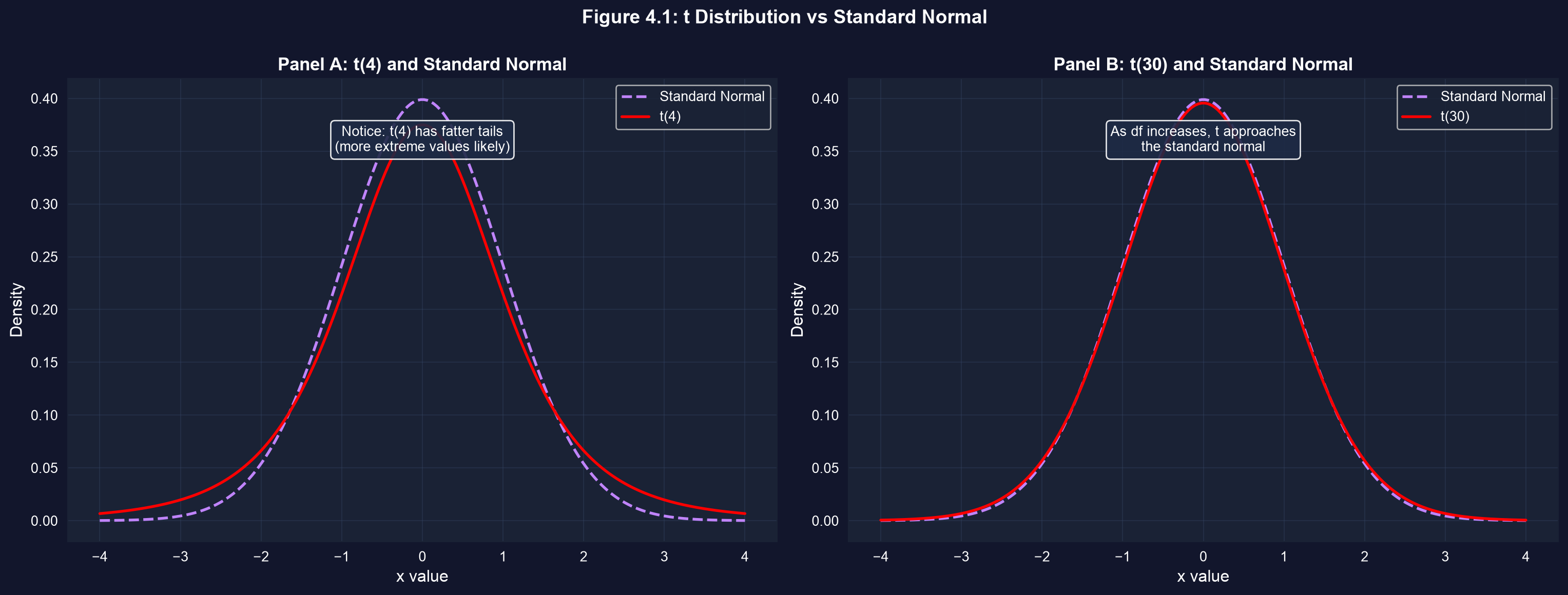
Panel A: \(t(4)\) has much fatter tails than the standard normal. Panel B: \(t(30)\) is already close to it.

With 4 degrees of freedom, values beyond ±2 are over twice as likely as under the normal.

Chapter Figure 4.1. Numbers computed for these slides: P(|T| > 2) is 11.6% for t(4), 5.5% for t(30) and 4.6% for the standard normal.

Code: critical values for different degrees of freedom

from scipy import stats                     # t and normal distributions
for df in [4, 9, 30, 99, 170]:              # degrees of freedom = n - 1
    t_crit = stats.t.ppf(0.975, df)         # 97.5th percentile: two-sided 5% cutoff
    print(f"df = {df:>3}: t critical = {t_crit:.3f}")
z_crit = stats.norm.ppf(0.975)              # the normal's cutoff, for comparison
print(f"normal:   z critical = {z_crit:.3f}")   # 1.960

↗ Try it in Colab

Computed for these slides; Exercise 3 of the chapter asks for the \(n = 10\) and \(n = 100\) cases.

Self-contained. ppf is the inverse CDF (percent-point function): it returns the cutoff with a given probability below it. 0.975 leaves 2.5% in the upper tail, which is the two-sided 5% critical value.

Output: by \(n = 171\) the \(t\) cutoff is almost the normal’s

Degrees of freedom	Sample size \(n\)	5% two-sided critical value
4	5	2.776
9	10	2.262
30	31	2.042
99	100	1.984
170	171	1.974
normal (\(\infty\))	—	1.960

For our sample the \(t\) critical value 1.974 is within 1% of 1.96, which is why the “estimate ± 2 SE” rule of thumb works.

The rule of thumb in the chapter: for n > 30, t(n−1, 0.025) ≈ 2. The correction matters only for small samples: with 10 observations the cutoff is 2.26, so using 1.96 would give intervals that are too narrow.

Section 4.3 · What values of \(\mu\) are plausible?

Confidence intervals · margin of error · the confidence–precision trade-off

Section 4.3: confidence intervals. Tools: the CI formula, the correct repeated-sampling interpretation, and the trade-off between confidence and width.

A confidence interval is estimate ± margin of error

\[\bar{x} \;\pm\; t_{n-1,\,\alpha/2} \times \text{se}(\bar{x})\]

• \(t_{n-1,\,\alpha/2}\): the critical value; for 95% confidence, \(\alpha = 0.05\) and we leave 2.5% in each tail
• Margin of error \(= t_{n-1,\,\alpha/2} \times \text{se}(\bar{x})\)
• Meaning: if we repeated the sampling many times, about 95% of the intervals built this way would contain \(\mu\)

The interval is random; \(\mu\) is fixed. The 95% describes the method, not this one interval.

Key Concept 4.3. The phrase “we are 95% confident” is shorthand for the repeated-sampling property. Rule of thumb for n > 30: x̄ ± 2 × se.

Code: the 95% confidence interval for mean earnings

import numpy as np                          # square roots
import pandas as pd                         # tabular data
from scipy import stats                     # t distribution
url = "https://raw.githubusercontent.com/quarcs-lab/data-open/master/AED/AED_EARNINGS.DTA"
earnings = pd.read_stata(url)["earnings"]   # 171 women, annual earnings
n = len(earnings)                           # sample size
mean_earnings = earnings.mean()             # x-bar
se_earnings = earnings.std(ddof=1) / np.sqrt(n)    # s / sqrt(n)
conf_level = 0.95                           # confidence level
alpha = 1 - conf_level                      # 0.05
t_crit = stats.t.ppf(1 - alpha/2, n - 1)    # critical value t(170, 0.025)
margin_of_error = t_crit * se_earnings      # half-width of the interval
print(mean_earnings - margin_of_error, mean_earnings + margin_of_error)  # the CI

↗ Try it in Colab

Self-contained. The chapter’s code is identical except that it reuses the variables from section 4.1.

Output: $37,559 to $45,266

Component	Value
Sample mean \(\bar{x}\)	$41,412.69
Standard error	$1,952.10
Critical value \(t_{170,\,0.025}\)	1.9740
Margin of error \(1.9740 \times 1{,}952.10\)	$3,853.48
95% confidence interval	[$37,559.21, $45,266.17]

Width $7,707 · computed with the \(t(170)\) distribution

The data are consistent with any population mean between about $37,600 and $45,300.

The interval excludes $36,000 and $46,000, so those values are implausible for μ, while $40,000 lies comfortably inside. That last fact will reappear as the result of the hypothesis test in section 4.4.

Reading the interval right

Correct

• 95% of intervals built this way, across repeated samples, contain \(\mu\)
• “We are 95% confident \(\mu\) is between $37,559 and $45,266”, as shorthand for the above
• The interval reflects sampling uncertainty only

Wrong

• “There is a 95% probability that \(\mu\) is in this interval”
• “95% of women earn between $37,559 and $45,266”
• “The interval contains 95% of the data”

The interval is about the mean. Individual earnings range from $1,050 to $172,000.

The second wrong reading is the most common in student work. Contrast the CI width (~$7,700) with the standard deviation of individual earnings (~$25,500).

Simulation: 39 of 40 intervals catch the mean

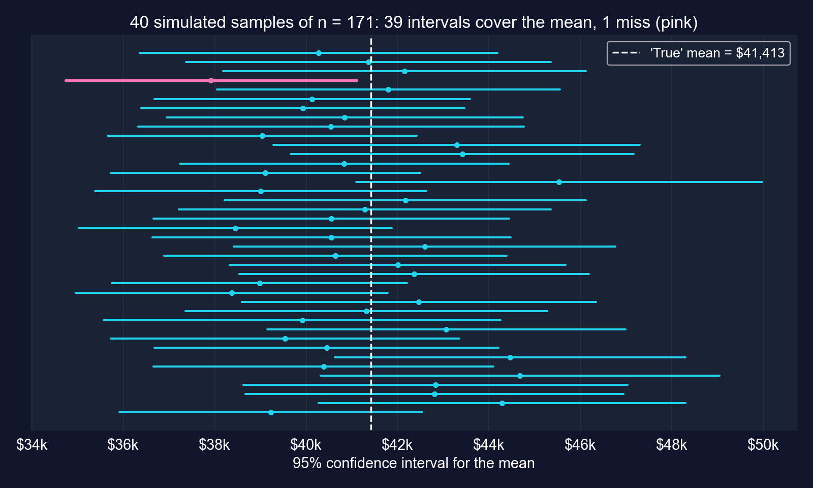
Each line is the 95% CI from one simulated sample of 171, resampled from the 171 earnings as if they were the population. The pink interval misses.

Each interval either contains \(\mu\) or it does not. The 95% is the long-run hit rate of the procedure.

Simulation made for these slides (seed 42), in the spirit of Exercise 8 of the chapter. We treat the 171 observed earnings as the population (so its mean $41,413 is the “true” μ) and draw 40 samples of 171 with replacement. With 40 intervals we expect about 2 misses; we got 1. Even though earnings are skewed, the t interval works well at n = 171.

Code: the same data at 90%, 95% and 99% confidence

# continues from the previous block (n, mean_earnings, se_earnings defined)
for conf in [0.90, 0.95, 0.99]:              # three confidence levels
    alpha = 1 - conf                        # tail probability, split in two
    t_crit = stats.t.ppf(1 - alpha/2, n - 1)    # larger for higher confidence
    ci_lower = mean_earnings - t_crit * se_earnings   # lower bound
    ci_upper = mean_earnings + t_crit * se_earnings   # upper bound
    width = ci_upper - ci_lower             # full width of the interval
    label = f"{conf*100:.0f}%"              # "90%", "95%", "99%"
    print(f"{label:<5} t={t_crit:.3f} [{ci_lower:,.2f}, {ci_upper:,.2f}] width {width:,.2f}")

↗ Try it in Colab

Only the critical value changes between the three lines; the estimate and its standard error are the same.

Output: more confidence costs width

Level	Critical value	Lower	Upper	Width
90%	1.654	$38,184.17	$44,641.21	$6,457.03
95%	1.974	$37,559.21	$45,266.17	$7,706.97
99%	2.605	$36,327.35	$46,498.03	$10,170.68

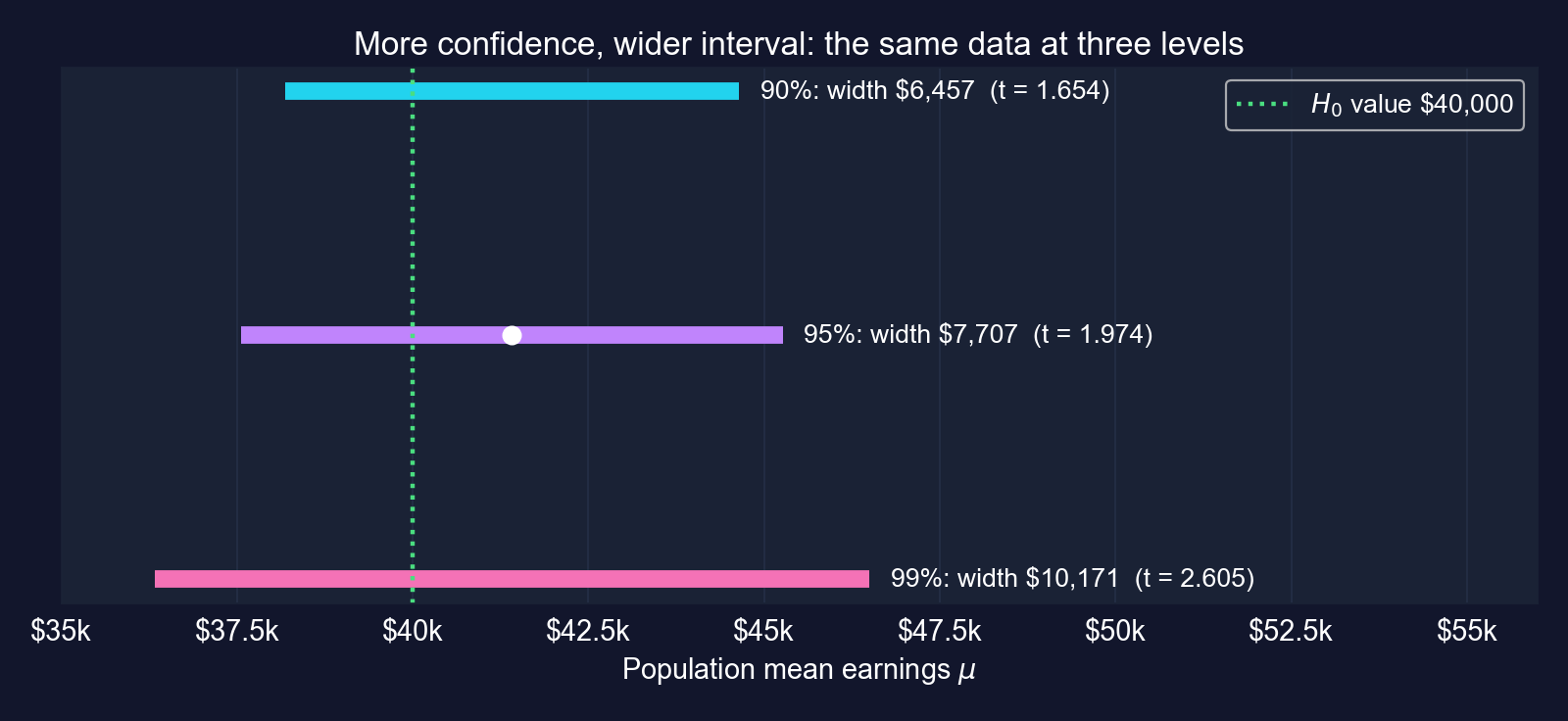
Going from 90% to 99% confidence makes the interval 58% wider. Only a larger sample buys both confidence and precision.

Width ratio 10,170.68 / 6,457.03 = 1.575. With n = 684 (4× larger) every interval would be about half as wide. 95% is the convention in economics; 99% is used when a false claim would be costly, 90% for exploratory work.

Section 4.4 · Is \(\mu = \$40{,}000\) credible?

Two-sided test · \(p\)-value · critical value · Type I and II errors · power

Section 4.4: the two-sided hypothesis test. Tools: H0 and Ha, the test statistic, the two equivalent decision rules, the duality with the confidence interval, the two kinds of error, and power.

A hypothesis test asks whether a claim survives the data

\[H_0: \mu = \mu_0 \quad \text{vs} \quad H_a: \mu \neq \mu_0 \qquad\qquad t = \frac{\bar{x} - \mu_0}{\text{se}(\bar{x})} \sim T(n-1) \text{ if } H_0 \text{ is true}\]

• \(p\)-value rule: \(p = 2 \times \Pr[T_{n-1} \geq |t|]\); reject \(H_0\) if \(p < \alpha\)
• Critical-value rule: reject \(H_0\) if \(|t| > t_{n-1,\,\alpha/2}\)
• The two rules always agree, and both agree with the CI: reject exactly when \(\mu_0\) lies outside the \(100(1-\alpha)\%\) interval

The test measures the gap between estimate and claim in standard errors, then asks how unusual that gap would be if the claim were true.

Key Concept 4.4. The example: H0: μ = $40,000 against Ha: μ ≠ $40,000 at α = 0.05.

Code: test \(H_0: \mu = \$40{,}000\)

import numpy as np                          # square roots
import pandas as pd                         # tabular data
from scipy import stats                     # t distribution
url = "https://raw.githubusercontent.com/quarcs-lab/data-open/master/AED/AED_EARNINGS.DTA"
earnings = pd.read_stata(url)["earnings"]   # 171 women, annual earnings
n, mean_earnings = len(earnings), earnings.mean()          # n and x-bar
se_earnings = earnings.std(ddof=1) / np.sqrt(n)            # standard error
mu0 = 40000                                 # hypothesized value under H0
t_stat = (mean_earnings - mu0) / se_earnings               # distance in SEs
p_value = 2 * (1 - stats.t.cdf(abs(t_stat), n - 1))        # two-sided p-value
t_crit_95 = stats.t.ppf(0.975, n - 1)       # critical value for alpha = 0.05
print(f"t = {t_stat:.4f}, p = {p_value:.4f}, critical = ±{t_crit_95:.4f}")
print("Reject H0" if p_value < 0.05 else "Do not reject H0")   # the decision

↗ Try it in Colab

Self-contained. stats.t.cdf(|t|, n − 1) is the probability below |t|; one minus it is the upper-tail area, doubled for a two-sided test.

Output: we do not reject \(H_0\)

	Value
\(\bar{x} - \mu_0\)	$1,412.69
Standard error	$1,952.10
\(t\)-statistic	0.7237
\(p\)-value (two-sided)	0.4703
Critical value	±1.9740
Decision at \(\alpha = 0.05\)	do not reject

\(\$40{,}000\) lies inside the 95% CI [$37,559, $45,266]

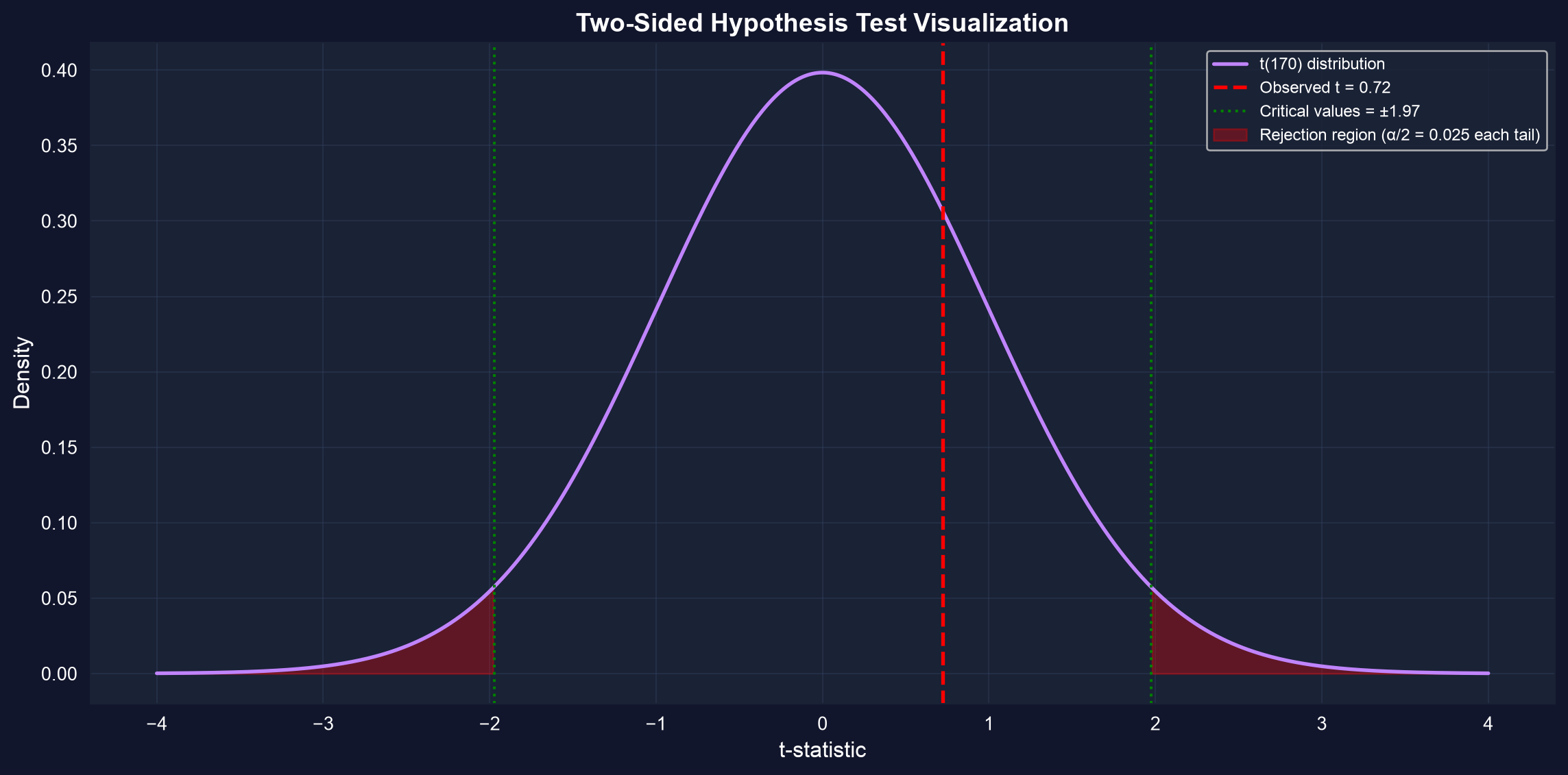
The sample mean is less than one standard error from $40,000, an ordinary amount of sampling noise.

Both rules agree: p = 0.4703 > 0.05, and |t| = 0.72 < 1.974. If μ really were $40,000, a sample mean at least this far from it (in either direction) would occur about 47% of the time.

What “do not reject” does and does not mean

• It means: the data are consistent with \(\mu = \$40{,}000\)
• It does not mean \(\mu = \$40{,}000\): $41,000, $43,000 or $45,000 are consistent too; the CI lists them all
• The \(p\)-value is not \(\Pr[H_0 \text{ true}]\): it is the probability of a gap at least this large if \(H_0\) were true
• The result could be a Type II error: a real difference that this sample is too small to detect

Key Concept 4.6: “fail to reject” is not “accept”. Report the confidence interval, which says how large a difference the data still allow.

Absence of evidence is not evidence of absence. The interval allows a population mean as much as $5,266 above $40,000.

Two ways to be wrong

	\(H_0\) true in reality	\(H_0\) false in reality
Reject \(H_0\)	Type I error (false alarm), probability \(\alpha\)	correct: power \(= 1-\beta\)
Do not reject \(H_0\)	correct, probability \(1-\alpha\)	Type II error (missed effect), probability \(\beta\)

• We choose \(\alpha\) (e.g. 0.05); \(\beta\) depends on \(n\), on the true gap, and on \(\alpha\)
• Lowering \(\alpha\) to 0.01 cuts false alarms but raises \(\beta\); raising it to 0.10 does the reverse
• Only a larger sample (or a larger true effect) lowers both at once

In the earnings test we did not reject, so the only mistake we could have made is a Type II error.

Choose α by the cost of each error. Medical trials, where a false claim is very costly, use α = 0.01; exploratory work sometimes uses 0.10. The usual target for power is 80% (β = 0.20).

Code: how likely was this test to detect a real gap?

# continues from the previous block (earnings, mu0 defined) — computed for these slides
s = earnings.std(ddof=1)                    # sample std dev, treated as known
for n_size in [171, 684]:                   # our sample, and 4x larger
    se = s / np.sqrt(n_size)                # standard error at this n
    df, c = n_size - 1, stats.t.ppf(0.975, n_size - 1)   # df and 5% critical value
    nc = (41412.69 - mu0) / se              # gap in SEs if the true mean were $41,412.69
    power = stats.nct.sf(c, df, nc) + stats.nct.cdf(-c, df, nc)   # P(|T| > c)
    print(f"n = {n_size}: power = {power:.3f}")   # probability of rejecting H0

↗ Try it in Colab

Power is not computed in the chapter, which discusses it in words; this calculation is added for the slides. If the true mean were $41,412.69, the test statistic would follow a noncentral t distribution with noncentrality (μ − μ0)/se. Power is the probability that |T| exceeds the critical value. stats.nct is scipy’s noncentral t.

Output: the test had little chance of detecting a $1,400 gap

True mean	\(n = 171\)	\(n = 684\)
$41,413	0.11	0.30
$45,000	0.72	1.00

Power of the two-sided 5% test of \(\mu = \$40{,}000\)

Smallest gap detected with 80% power:

• $5,500 with \(n = 171\)
• $2,738 with \(n = 684\)

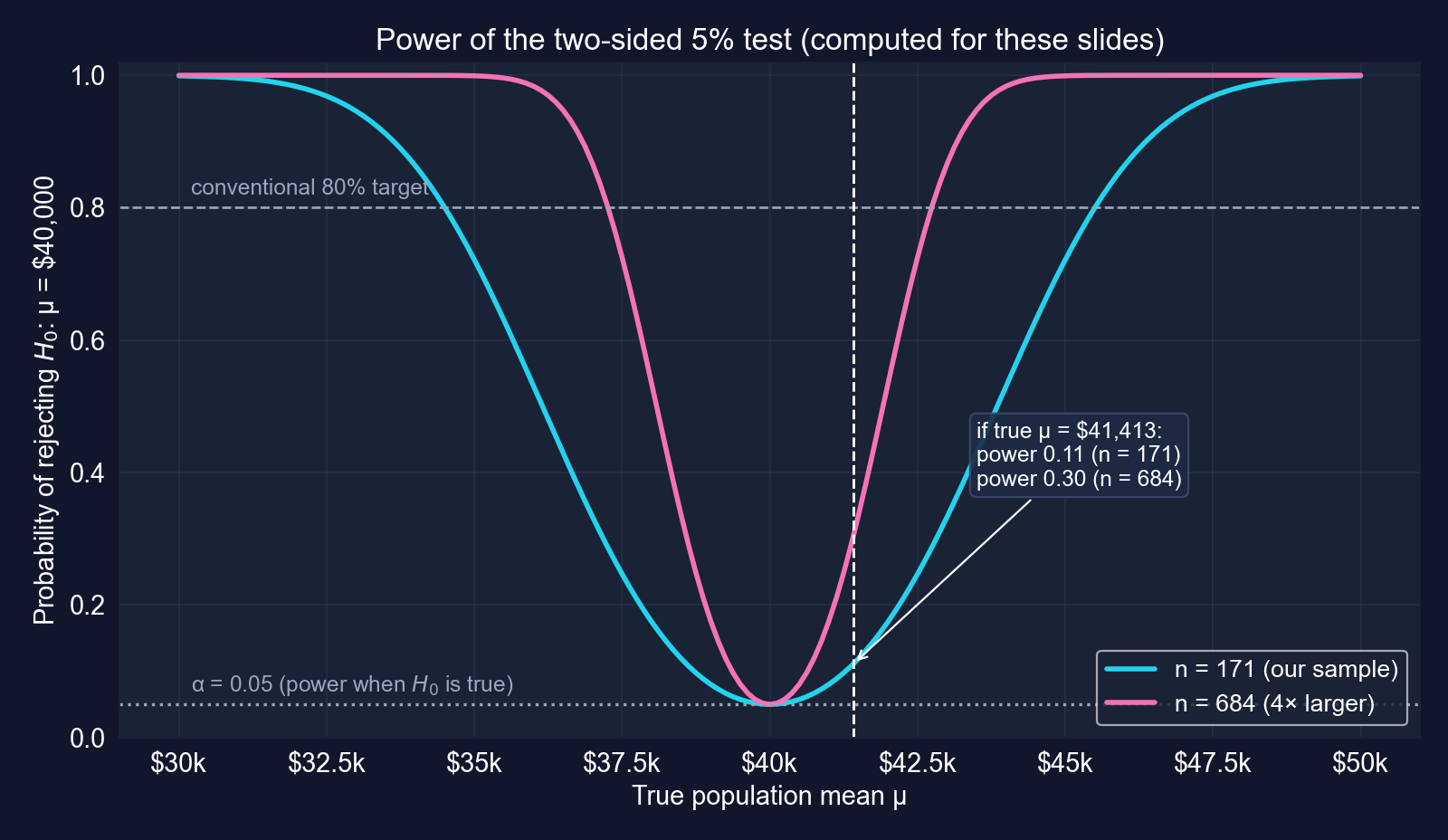
Even if $41,413 were the truth, the test would reject only 11% of the time. Failing to reject here says more about the sample size than about \(\mu\).

Computed for these slides. The chapter’s own reasoning (Key Concepts glossary): quadrupling the sample would double t to about 1.45, still below 1.96. The power curve makes that precise: with 684 women the power at μ = $41,413 is still only 0.30. At n = 684, μ = $45,000 the power is 0.9992, shown as 1.00. Power equals α = 0.05 exactly at μ = μ0.

Section 4.5 · Three tests on real questions

Gas prices · male earnings · GDP growth

Section 4.5 applies the same two-sided test to three new datasets, and gives three very different answers. Each is a chance to ask the thread’s three questions: is it real, does it matter, could we tell?

Same test, three datasets, three different lessons

Example	Data	\(H_0\)	\(t\)	\(p\)	Decision	Lesson
Gas prices	32 stations, Yolo County	\(\mu = \$3.81\)	−5.26	< 0.0001	reject	a small gap can be very precise
Male earnings	191 men aged 30	\(\mu = \$50{,}000\)	0.50	0.617	do not reject	heavy tails, imprecise mean
GDP growth	241 quarters, U.S.	\(\mu = 2.0\%\)	−0.07	0.946	do not reject	dependent data, SE too small

One recipe, three verdicts. The interpretation always depends on the data behind the numbers.

Key Concept 4.7: the testing pattern is the same across applications; meaning comes from context. The next slides take each example through its own arc.

Gas prices: are Yolo County prices different from the state’s?

Question. Is the mean price at Yolo County gas stations different from the California average of $3.81 per gallon?

Data. AED_GASPRICE.DTA: 32 stations in three cities (West Sacramento 15, Davis 10, Woodland 7).

\[H_0: \mu = 3.81 \qquad H_a: \mu \neq 3.81 \qquad t \text{ with } 31 \text{ degrees of freedom}\]

A two-sided question: prices could be higher or lower than the state average.

The chapter frames this as the classic statistical-vs-practical significance example. The critical value with 31 degrees of freedom is 2.04, a little above 1.96 because the sample is small.

Code: test the gas-price claim

import numpy as np                          # square roots
import pandas as pd                         # tabular data
from scipy import stats                     # t distribution
url = "https://raw.githubusercontent.com/quarcs-lab/data-open/master/AED/AED_GASPRICE.DTA"
price = pd.read_stata(url)["price"]         # price per gallon at 32 stations
mean_price = price.mean()                   # sample mean
std_price = price.std(ddof=1)               # sample std dev
n_price = len(price)                        # 32 stations
se_price = std_price / np.sqrt(n_price)     # standard error
mu0_price = 3.81                            # California state average
t_stat_price = (mean_price - mu0_price) / se_price               # distance in SEs
p_value_price = 2 * (1 - stats.t.cdf(abs(t_stat_price), n_price - 1))   # two-sided p
print(f"mean {mean_price:.4f}, se {se_price:.4f}, t {t_stat_price:.4f}, p {p_value_price:.6f}")

↗ Try it in Colab

Self-contained; the chapter’s code.

Output: a 14-cent gap, more than five standard errors wide

	Value
\(n\)	32
Mean	$3.6697
Std. dev.	$0.1510
Std. error	$0.0267
\(t\)	−5.2577
\(p\) (two-sided)	0.00001
95% CI	[$3.615, $3.724]

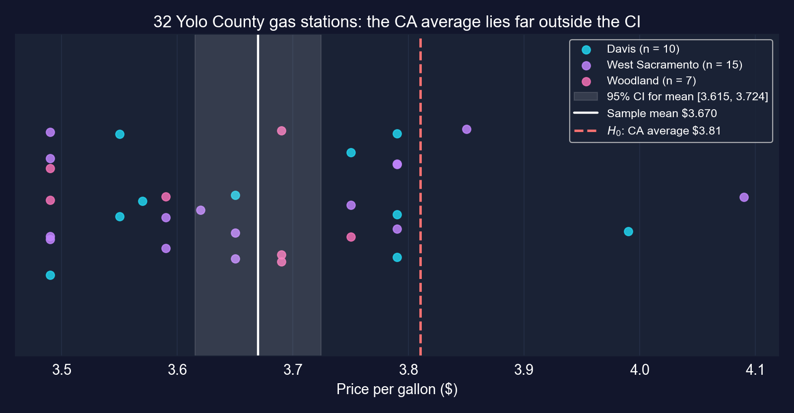
Reject \(H_0\): Yolo County prices are lower than the state average, and $3.81 lies far outside the 95% CI.

p = 0.0000103, which the chapter prints as 0.0000 and describes as < 0.0001. The 95% CI (computed for these slides, with t(31) = 2.04) runs from $3.615 to $3.724. The figure shows every station; the white band is the CI for the mean, not for individual prices.

Is it real, and does it matter?

• Real? Yes: \(t = -5.26\). Prices barely vary across stations (SD 15¢), so the SE is under 3¢ and a 14-cent gap is easy to detect
• Does it matter? 14¢ × 15 gallons = $2.10 per tank; with 52 fill-ups a year, about $109 a year: meaningful for a household
• Could we tell? Yes, easily: high power from a small SE, even with only 32 stations

Key Concept 4.5: a small difference can be highly significant when it is precisely measured. Significance is about the gap relative to its SE, not its size.

The chapter’s practical-significance arithmetic uses the rounded 14¢ gap: 0.14 × 15 = $2.10; × 52 = $109.20. With the unrounded gap of 14.03¢ the yearly figure is $109.44.

Caveats on the gas-price test

• Sampling: 32 stations in three cities, not a random sample of all county stations; West Sacramento alone is almost half the sample
• Timing: one snapshot; the state average must refer to the same period for the comparison to be fair
• The benchmark is itself an estimate: $3.81 is treated as a known constant
• The test says Yolo prices are lower on average; one station sells at $4.09

A \(p\)-value of 0.00001 settles the sampling-noise question only. It cannot fix a non-random sample or a mismatched benchmark.

Standard caveats. The city counts come from the data’s city variable. If prices were collected on one day and the state average refers to a monthly mean, part of the gap could reflect timing rather than location.

Male earnings: do 30-year-old men earn more than $50,000?

Data. AED_EARNINGSMALE.DTA: 191 men aged 30 working full time, 2010.

The chapter’s test is two-sided:

\[H_0: \mu = 50{,}000 \qquad H_a: \mu \neq 50{,}000\]

The question is directional (“more than”), so its natural form is one-sided; the chapter defers that to section 4.6. These slides report both.

The chapter computes the two-sided test here and notes that a one-sided test is more appropriate. Section 4.6 then runs its one-sided example on the female earnings data instead, so the one-sided p-value for men is computed for these slides.

Code: test the male-earnings claim

import numpy as np                          # square roots
import pandas as pd                         # tabular data
from scipy import stats                     # t distribution
url = "https://raw.githubusercontent.com/quarcs-lab/data-open/master/AED/AED_EARNINGSMALE.DTA"
earnings_male = pd.read_stata(url)["earnings"]   # 191 men, annual earnings
mean_male = earnings_male.mean()            # sample mean
std_male = earnings_male.std(ddof=1)        # sample std dev
n_male = len(earnings_male)                 # 191
se_male = std_male / np.sqrt(n_male)        # standard error
mu0_male = 50000                            # hypothesized value
t_stat_male = (mean_male - mu0_male) / se_male                      # distance in SEs
p_value_male = 2 * (1 - stats.t.cdf(abs(t_stat_male), n_male - 1)) # two-sided p
p_upper_male = 1 - stats.t.cdf(t_stat_male, n_male - 1)             # one-sided (Ha: mu > 50,000)
print(f"mean {mean_male:,.2f}, se {se_male:,.2f}, t {t_stat_male:.4f}")   # estimate and t
print(f"two-sided p {p_value_male:.4f}, one-sided p {p_upper_male:.4f}")   # both p-values

↗ Try it in Colab

Self-contained. The last computed line (p_upper_male) is added for these slides; the rest is the chapter’s code.

Output: a $2,354 gap buried in a $4,706 standard error

	Value
\(n\)	191
Mean	$52,353.93
Median	$38,000
Std. dev.	$65,034.74
Std. error	$4,705.75
\(t\)	0.5002
\(p\) (two-sided)	0.6175
\(p\) (one-sided, \(H_a: \mu > 50{,}000\))	0.3087
95% CI	[$43,072, $61,636]

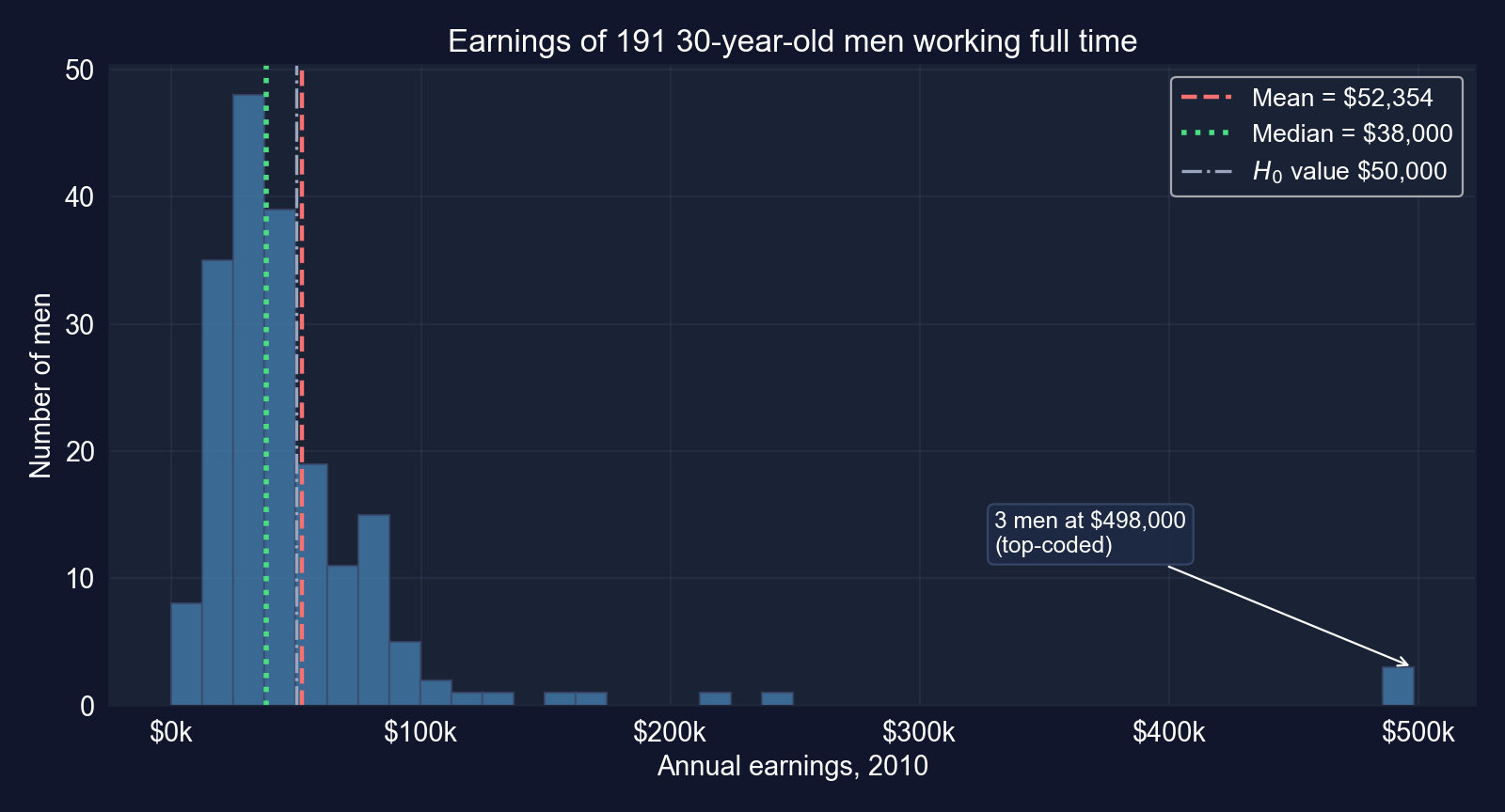
Do not reject either way. Whether men’s mean earnings exceed $50,000 is unresolved; the CI runs from $43,100 to $61,600.

One-sided p and the 95% CI are computed for these slides. The one-sided p-value is half the two-sided one, because t is positive (in the direction of Ha).

Why the male-earnings test has so little power

• Heavy tails: three men are recorded at $498,000, the data’s top code, and one at $1; the SD ($65,035) is 2.5× the women’s
• The mean ($52,354) sits far above the median ($38,000); without the three top-coded men it would be $45,243
• A large SD means a large SE, so a gap of $2,354 is only half a standard error

Not rejecting here is mostly a statement about noise. A mean driven by three people is a fragile target for inference.

The chapter lists three possible reasons for not rejecting: H0 true, insufficient power, high variability. The data point strongly to the third. The mean excluding the three top-coded observations is a simple descriptive check computed for these slides, not a recommended estimator; with top coding the true mean is, if anything, higher than the sample mean. Medians and other robust summaries come later in the book.

GDP growth: has U.S. growth averaged 2% a year?

Data. AED_REALGDPPC.DTA: U.S. real GDP per capita, quarterly, 1959Q1–2020Q1. The variable growth is the year-over-year growth rate, so it starts in 1960Q1: 241 quarterly observations.

\[H_0: \mu = 2.0 \qquad H_a: \mu \neq 2.0 \quad (\text{percent per year})\]

Note what the 241 observations are: overlapping four-quarter growth rates, not 241 separate years.

Verified from the data: growth equals 100 × (realgdppc_t / realgdppc_(t−4) − 1). Each observation shares three of its four quarters with the previous one, so consecutive observations are strongly correlated. So the 241 observations are not 241 independent years; the data cover about 60 years.

Code: test the 2% benchmark

import numpy as np                          # square roots
import pandas as pd                         # tabular data
from scipy import stats                     # t distribution
url = "https://raw.githubusercontent.com/quarcs-lab/data-open/master/AED/AED_REALGDPPC.DTA"
growth = pd.read_stata(url)["growth"].dropna()   # first 4 quarters have no YoY growth
mean_growth = growth.mean()                 # average growth, % per year
std_growth = growth.std(ddof=1)             # sample std dev
n_growth = len(growth)                      # 241 quarters
se_growth = std_growth / np.sqrt(n_growth)  # SE, assuming independent observations
mu0_growth = 2.0                            # benchmark under H0
t_stat_growth = (mean_growth - mu0_growth) / se_growth                    # distance in SEs
p_value_growth = 2 * (1 - stats.t.cdf(abs(t_stat_growth), n_growth - 1))  # two-sided p
print(f"mean {mean_growth:.4f}, se {se_growth:.4f}, t {t_stat_growth:.4f}, p {p_value_growth:.4f}")
print(f"lag-1 autocorrelation {growth.autocorr(1):.2f}")   # neighbouring quarters move together

↗ Try it in Colab

Self-contained; the chapter’s code, plus growth.autocorr(1), the correlation between each quarter’s value and the previous quarter’s, added for these slides.

Output: the mean is 1.99%, but the observations are not independent

	Value
\(n\) (quarters)	241
Mean	1.9905%
Std. dev.	2.1781
Std. error (i.i.d.)	0.1403
\(t\)	−0.0680
\(p\) (two-sided)	0.9458
95% CI (i.i.d.)	[1.71%, 2.27%]
Lag-1 autocorrelation	0.87

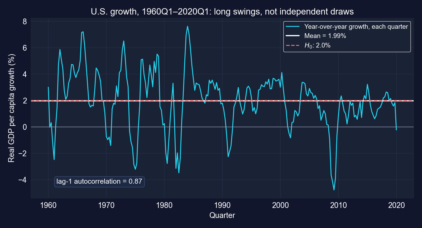
Do not reject 2%. But with a lag-1 correlation of 0.87, the i.i.d. standard error understates the true uncertainty.

The CI and the autocorrelation are computed for these slides. The figure shows long swings (recessions in 1974–75, 1980–82, 2008–09), not independent draws around a mean. A rough rule of thumb for an AR(1) series gives an “effective” sample of n(1 − ρ)/(1 + ρ) ≈ 17 independent observations rather than 241; the right standard error (HAC, Chapters 12 and 17) would be several times larger than 0.14.

Not rejecting does not “validate” the 2% benchmark

• Real? No evidence of a difference from 2%, so the result is “consistent with 2%”, not “2% confirmed”
• Could we tell? Less than the output suggests: the SE of 0.14 assumes 241 independent observations, but neighbouring quarters overlap
• Does it matter? Yes: 1.5% versus 2.5% growth compounds into very different living standards over 60 years

Key Concept 4.6 applies here too: the data fail to reject 2%, but that does not show the long-run rate is 2%. With dependent data, report a wider interval.

Failing to reject never confirms H0, and the 241 overlapping observations carry far less information than 241 independent draws. The chapter makes both points (non-rejection is not proof; with a lag-1 autocorrelation of about 0.87 the i.i.d. t-test is only approximate) and points to Chapter 17; these slides put that caveat up front.

Section 4.6 · Does \(\mu\) exceed $40,000?

One-sided (directional) tests · upper and lower tails

Section 4.6: one-sided tests. Tools: upper- and lower-tailed hypotheses, one-tail p-values and critical values, and when a one-sided test is legitimate.

A directional claim puts the whole rejection region in one tail

Test	\(H_0\)	\(H_a\)	\(p\)-value	Reject if
Upper-tailed	\(\mu \leq \mu^*\)	\(\mu > \mu^*\)	\(\Pr[T_{n-1} \geq t]\)	\(t > t_{n-1,\,\alpha}\)
Lower-tailed	\(\mu \geq \mu^*\)	\(\mu < \mu^*\)	\(\Pr[T_{n-1} \leq t]\)	\(t < -t_{n-1,\,\alpha}\)
Two-sided	\(\mu = \mu^*\)	\(\mu \neq \mu^*\)	\(2\Pr[T_{n-1} \geq \lvert t \rvert]\)	\(\lvert t \rvert > t_{n-1,\,\alpha/2}\)

• The claim we want to establish goes in \(H_a\)
• All of \(\alpha\) sits in one tail, so the critical value is smaller: 1.654 instead of 1.974 for \(n = 171\)
• If \(t\) has the sign \(H_a\) predicts, the one-sided \(p\) is half the two-sided \(p\); if not, it is above 0.5

One-sided tests are more powerful in the chosen direction and blind in the other.

Key Concept 4.8. The “half the two-sided p-value” rule holds only when the estimate falls on the side Ha predicts. Case Study 1, Task 4 shows the opposite case.

Code: upper-tailed test of \(H_a: \mu > \$40{,}000\)

import numpy as np                          # square roots
import pandas as pd                         # tabular data
from scipy import stats                     # t distribution
url = "https://raw.githubusercontent.com/quarcs-lab/data-open/master/AED/AED_EARNINGS.DTA"
earnings = pd.read_stata(url)["earnings"]   # 171 women, annual earnings
n, se_earnings = len(earnings), earnings.std(ddof=1) / np.sqrt(len(earnings))   # n and SE
mu0 = 40000                                 # H0: mu <= 40,000
t_stat = (earnings.mean() - mu0) / se_earnings     # same t as the two-sided test
p_value_upper = 1 - stats.t.cdf(t_stat, n - 1)     # upper-tail area only
t_crit_upper = stats.t.ppf(0.95, n - 1)     # all 5% in the upper tail
print(f"t = {t_stat:.4f}, one-sided p = {p_value_upper:.4f}, critical = {t_crit_upper:.4f}")

↗ Try it in Colab

Self-contained. Note 0.95 instead of 0.975 in the critical value: no splitting of α between two tails.

Output: still no rejection, even with the lower bar

	One-sided	Two-sided
\(t\)-statistic	0.7237	0.7237
\(p\)-value	0.2351	0.4703
Critical value	1.6539	±1.9740
Decision	do not reject	do not reject

\(0.2351 = 0.4703 / 2\), because \(t > 0\) points the way \(H_a\) predicts

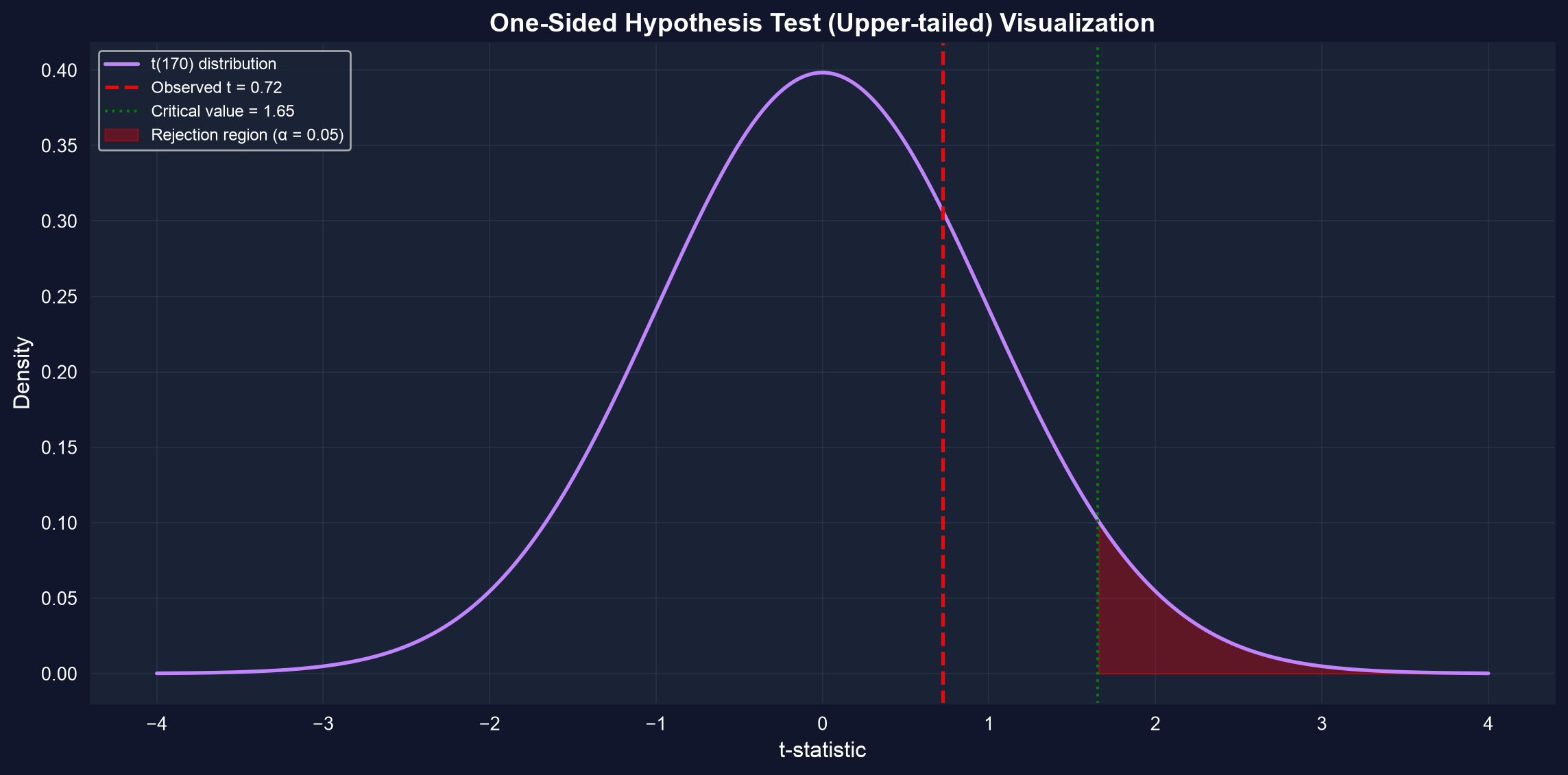
We cannot conclude that mean earnings exceed $40,000. The gap is small relative to its SE, whichever test we use.

The figure is the chapter’s one-sided visualization: the shaded upper tail holds all 5%, cut off at 1.654. The observed t = 0.72 is well short of it.

When is a one-sided test legitimate?

Use it when

• theory or policy fixes the direction before seeing the data
• only one direction would change a decision (a drug better than placebo; a policy that raises income)

Avoid it when

• either direction would be interesting
• the field reports two-sided tests (economics usually does)
• you switch after seeing a two-sided \(p = 0.08\) to get a one-sided \(p = 0.04\): that is \(p\)-hacking

Decide the direction before looking at the data. A one-sided test chosen afterwards has a true false-alarm rate of 10%, not 5%.

If a researcher picks the tail after seeing which way the estimate points, they effectively run a two-sided test at the 10% level while reporting 5%. That is why the choice must be pre-specified.

Section 4.7 · Is the race tied?

Proportions · binary data · the \(z\) test

Section 4.7: proportions. Tools: the sample proportion as a mean of 0/1 data, its standard error, the normal-based CI and z test.

A proportion is just the mean of 0/1 data

\[\hat{p} = \bar{x} = \frac{\#\text{yes}}{n} \qquad \text{se}(\hat{p}) = \sqrt{\frac{\hat{p}(1-\hat{p})}{n}} \qquad \text{CI: } \hat{p} \pm z_{\alpha/2}\,\text{se}(\hat{p})\]

• Code each voter 1 (Democrat) or 0 (not): \(\hat{p}\) is the sample mean and the variance is \(\hat{p}(1-\hat{p})\)
• With large \(n\) (rule of thumb: \(n\hat{p} \geq 10\) and \(n(1-\hat{p}) \geq 10\)) use the normal critical value, 1.96
• To test \(H_0: p = p_0\), use the SE implied by \(H_0\): \(z = (\hat{p} - p_0)/\sqrt{p_0(1-p_0)/n}\)

Everything learned about means carries over; only the SE formula changes.

Key Concept 4.9. Two different SEs appear: the CI uses p̂(1 − p̂)/n, the test uses p0(1 − p0)/n because under H0 we know the variance. With p̂ = 0.521 and p0 = 0.5 they are almost identical (0.01646 vs 0.01648).

Code: 480 of 921 voters intend to vote Democrat

import numpy as np                          # square roots
from scipy import stats                     # normal distribution
n_total = 921                               # voters polled
n_success = 480                             # intend to vote Democrat
p_hat = n_success / n_total                 # sample proportion
se_prop = np.sqrt(p_hat * (1 - p_hat) / n_total)   # SE at p-hat (for the CI)
z_crit = 1.96                               # normal critical value, 95%
ci_lower_prop = p_hat - z_crit * se_prop    # lower bound
ci_upper_prop = p_hat + z_crit * se_prop    # upper bound
p0 = 0.50                                   # H0: tied race
se_under_h0 = np.sqrt(p0 * (1 - p0) / n_total)     # SE implied by H0
z_stat = (p_hat - p0) / se_under_h0         # z statistic
p_value_prop = 2 * (1 - stats.norm.cdf(abs(z_stat)))   # two-sided p (normal)
print(f"p_hat {p_hat:.4f}, se {se_prop:.4f}")   # estimate and its SE
print(f"95% CI [{ci_lower_prop:.4f}, {ci_upper_prop:.4f}]")   # interval
print(f"z {z_stat:.4f}, p {p_value_prop:.4f}")   # test of a tied race

↗ Try it in Colab

Self-contained; the chapter’s code. No data file: the poll is given as two counts.

Output: 52.1%, but a tie cannot be ruled out

	Value
\(\hat{p}\)	0.5212
SE	0.0165
95% CI	[0.4889, 0.5534]
Margin of error	±3.2 pp
\(z\) (vs 0.50)	1.2851
\(p\)-value	0.1988

\(n\hat{p} = 480\), \(n(1-\hat{p}) = 441\): both far above 10

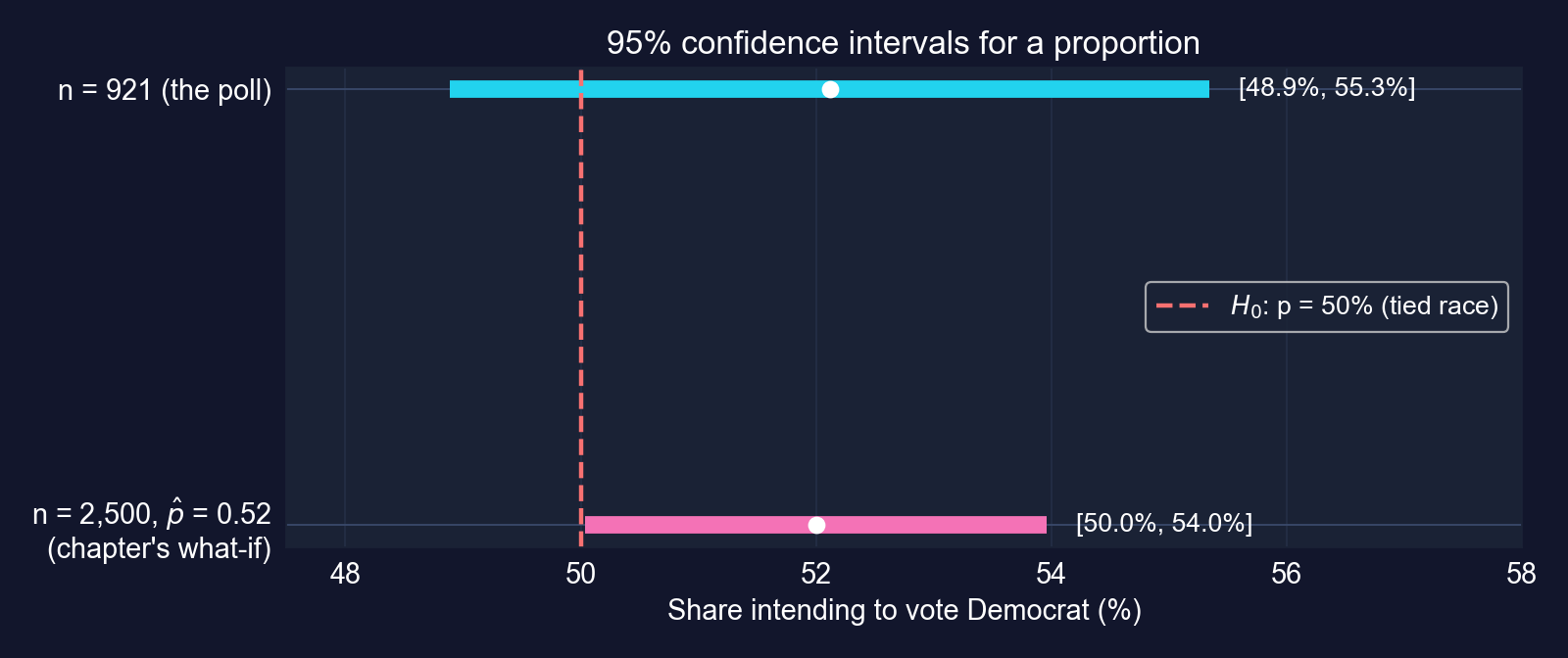
Do not reject a tied race: the CI [48.9%, 55.3%] contains 50%. The lead is 2.1 percentage points with a ±3.2-point margin.

z = 1.29: the sample proportion is 1.29 standard errors above 50%. About a 20% chance of a gap at least this large if the race were truly tied. The lower bar in the figure is the chapter’s what-if, discussed on the next slide.

Same share, bigger poll: when does 52% become significant?

• The chapter’s what-if: the same share, 52%, from 2,500 voters
• SE falls to 0.010; 95% CI [50.0%, 54.0%]; \(z = 2.00\), \(p = 0.045\): significant at 5%, only just
• With the exact \(\hat{p} = 0.5212\) instead of 0.52: \(z = 2.12\), \(p = 0.034\)

Nothing about the voters changed, only the sample size. Statistical significance is as much about \(n\) as about the effect.

The chapter’s numbers use p̂ rounded to 0.52; the exact-p̂ version is computed for these slides. Either way the lower CI bound sits a hair above 50% (50.04% with p̂ = 0.52), so “significant” here is a knife-edge call. Practical side: a 2-point lead matters a great deal in an election, so this is a case where the effect may matter even when we cannot yet tell.

Caveats on polls

• The SE covers sampling error only; non-response and people who change their minds are not in it
• “Intend to vote” is not “will vote”: the population of voters differs from the population polled
• The normal approximation needs \(n\hat{p}\) and \(n(1-\hat{p})\) both large; for rare events use exact methods

The reported margin of error (±3.2 points) is a floor on the real uncertainty, not a ceiling.

Standard caveats for proportions from surveys. The same logic applies to employment rates, approval ratings or market shares.

Case Study 1 · Has world labor productivity changed?

Mendez convergence-clubs data · 108 countries · 1990 and 2014 · six tasks

Case Study 1 applies every tool of the chapter to cross-country productivity. The chapter gives the tasks as fill-in templates and outlines without output; every task is run here, with the blanks filled in, and its output reported. Results not printed in the chapter are therefore all “computed for these slides”.

The question: productivity growth and gaps across countries

Data. Mendez (2020) convergence-clubs panel: 108 countries × 25 years (1990–2014) = 2,700 observations. We use labor productivity lp (output per worker, in dollars) for 1990 and 2014, and region.

Task	Question	Tool (section)
1	Range of mean productivity in 2014?	CI, 95% vs 99% (4.3)
2	Did mean productivity change, 1990 → 2014?	two-sample and paired \(t\) tests (4.4)
3	Is Africa below Europe?	two-sample test, CI for a difference
4	Does the 2014 mean exceed $50,000?	one-sided test (4.6)
5	Did more than half of countries grow?	proportions (4.7)
6	Which regions differ?	many tests, multiple testing

Six tasks, one dataset: the chapter’s whole toolkit on a development question.

Economic context: the convergence hypothesis says poorer countries should grow faster than richer ones. The tasks test levels and changes of mean productivity; they do not test convergence directly, which needs growth-on-initial-level regressions (later chapters).

Code: load the panel and extract the two cross-sections

import numpy as np                          # square roots
import pandas as pd                         # tabular data
from scipy import stats                     # t and normal distributions
import matplotlib.pyplot as plt             # plots
url = ("https://raw.githubusercontent.com/quarcs-lab/"            # Mendez (2020) repository
       "mendez2020-convergence-clubs-code-data/master/assets/dat.csv")
df = pd.read_csv(url).set_index(["country", "year"])     # panel indexed by country-year
lp_1990 = df.loc[df.index.get_level_values("year") == 1990, "lp"]   # productivity, 1990
lp_2014 = df.loc[df.index.get_level_values("year") == 2014, "lp"]   # productivity, 2014
print(f"Observations: {len(df):,}; countries: {df.index.get_level_values('country').nunique()}")
print(f"1990: n={len(lp_1990)}, mean={lp_1990.mean():,.0f}, std={lp_1990.std():,.0f}")
print(f"2014: n={len(lp_2014)}, mean={lp_2014.mean():,.0f}, std={lp_2014.std():,.0f}")

↗ Try it in Colab

Self-contained; the chapter’s loading cell. Every later block in this case study continues from here. pandas .std() uses ddof=1 by default, i.e. the sample standard deviation.

Output: the mean rose, and so did the spread

	1990	2014
Countries	108	108
Mean	$23,224	$40,977
Median	$16,985	$32,781
Std. dev.	$20,089	$33,853
Std. error	$1,933	$3,258

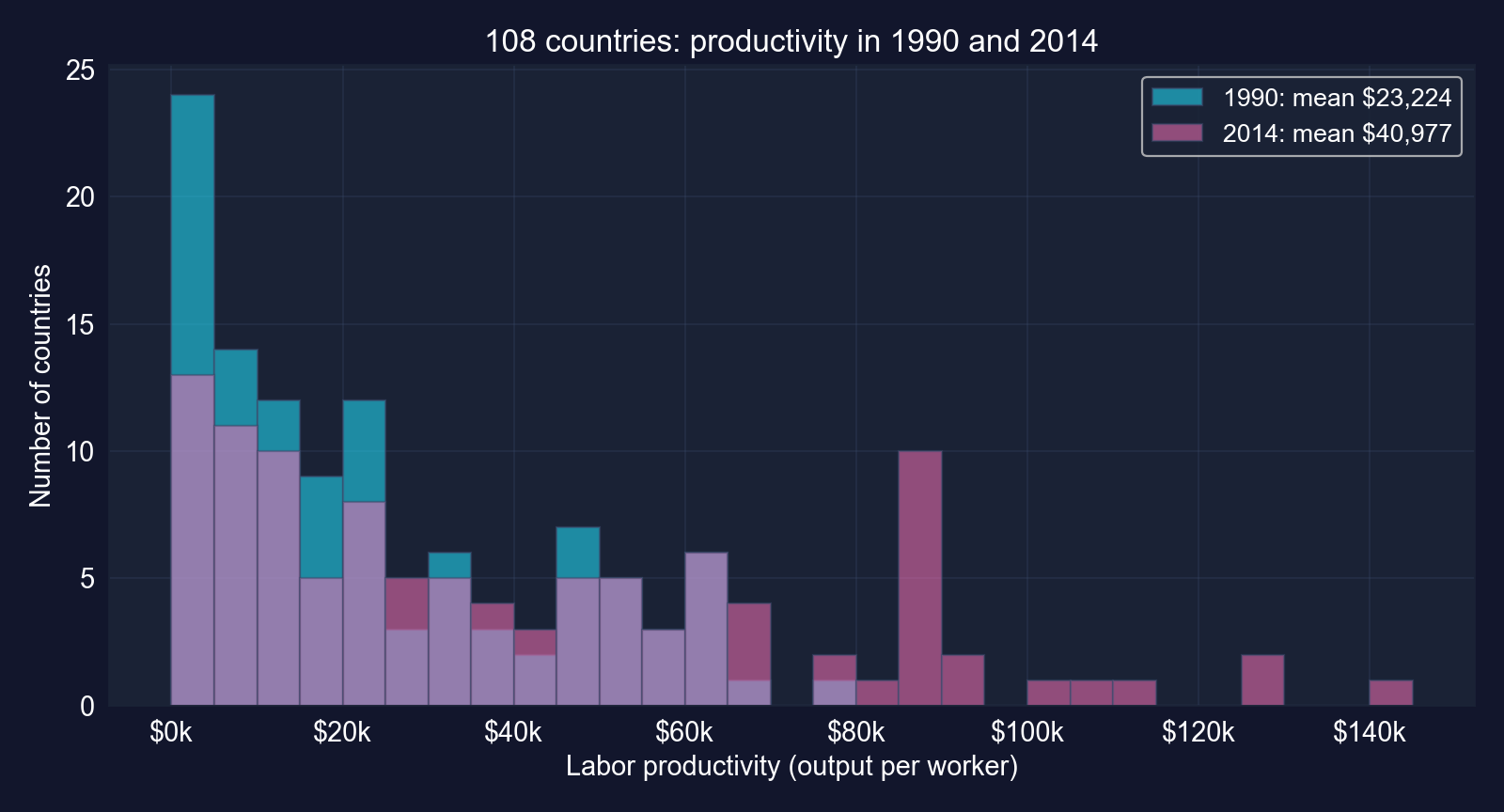
Mean productivity rose 76% and the cross-country standard deviation rose 69%. Both distributions are right-skewed.

Computed for these slides from the chapter’s loading cell. A rising SD of levels is not by itself evidence for or against convergence, which is usually studied in logs (a constant percentage gap means a growing dollar gap). Keep the two questions apart: these tasks are about means.

Task 1 code: 95% and 99% CIs for 2014 (template filled)

# continues from the previous block
n_2014 = len(lp_2014)                       # 108 countries
mean_2014 = lp_2014.mean()                  # blank 1: sample mean
std_2014 = lp_2014.std()                    # blank 2: sample std dev
se_2014 = std_2014 / np.sqrt(n_2014)        # standard error
t_crit_95 = stats.t.ppf(1 - 0.05/2, df=n_2014 - 1)   # blank 3: df = n - 1
me_95 = t_crit_95 * se_2014                 # 95% margin of error
ci_95 = (mean_2014 - me_95, mean_2014 + me_95)       # blanks 4-5: the bounds
t_crit_99 = stats.t.ppf(1 - 0.01/2, df=n_2014 - 1)   # 99% critical value
me_99 = t_crit_99 * se_2014                 # 99% margin of error: wider
ci_99 = (mean_2014 - me_99, mean_2014 + me_99)       # 99% bounds
se_1990 = lp_1990.std() / np.sqrt(len(lp_1990))      # 1990 for comparison
me_1990 = stats.t.ppf(0.975, df=len(lp_1990) - 1) * se_1990   # 1990 margin
print(ci_95, ci_99, 2 * me_95, 2 * me_1990)          # bounds and widths

↗ Try it in Colab

The chapter’s Task 1 template with its six blanks filled: mean, std, df = n − 1, the two bounds, and “wider”. The answer to the last blank: the 99% CI is wider than the 95% CI.

Task 1 output: the 2014 interval is wide, and wider than 1990’s

	Mean	95% CI	95% width	99% CI	99% width
2014	$40,977	[$34,519, $47,435]	$12,915	[$32,434, $49,520]	$17,086
1990	$23,224	[$19,392, $27,056]	$7,664	[$18,154, $28,293]	$10,139

\(t_{107,\,0.025} = 1.982\), \(t_{107,\,0.005} = 2.623\); \(n = 108\) in both years · computed for these slides

• The 99% CI is wider (the template’s last blank): more confidence costs width
• The 2014 interval is 69% wider than 1990’s because countries became more dispersed, with the same \(n\)
• The two 95% intervals do not overlap: a first hint that the mean changed

Precision depends on dispersion as well as sample size: same 108 countries, much less precise mean.

Width ratio 12,915/7,664 = 1.685, equal to the ratio of standard deviations (33,853/20,089) because n is the same. Non-overlapping intervals imply a significant difference, but overlapping ones would not imply the opposite; Task 2 runs the proper test.

Task 2 code: did mean productivity change? Two tests

# continues from the previous block
se_1990, se_2014 = lp_1990.std() / np.sqrt(108), lp_2014.std() / np.sqrt(108)   # each SE
se_diff = np.sqrt(se_1990**2 + se_2014**2)  # blanks 1-2: SE of the difference
t_stat = (lp_2014.mean() - lp_1990.mean()) / se_diff   # blanks 3-4: Welch t
t_scipy, p_scipy = stats.ttest_ind(lp_2014, lp_1990, equal_var=False)   # blanks 5-6
print(f"Welch: diff {lp_2014.mean() - lp_1990.mean():,.0f}, se {se_diff:,.0f}")
print(f"       t {t_scipy:.3f}, p {p_scipy:.2e}")              # blank 7: Reject
# computed for these slides: the same 108 countries appear in both years
x14, x90 = lp_2014.droplevel("year"), lp_1990.droplevel("year")   # align by country
t_pair, p_pair = stats.ttest_rel(x14, x90)  # paired test = one-sample t on the changes
change = x14 - x90                          # within-country change
print(f"Paired: mean change {change.mean():,.0f}, se {change.std() / np.sqrt(108):,.0f}")
print(f"        t {t_pair:.3f}, p {p_pair:.2e}")   # paired test result

↗ Try it in Colab

The first part is the chapter’s Task 2 template, filled in (Welch’s unequal-variance test). The chapter’s own discussion question notes that the 1990 and 2014 samples contain the same countries and suggests a paired test; the paired test is computed for these slides. droplevel(“year”) removes the year from the index so that the two Series line up by country.

Task 2 output: same verdict, but the paired test is far sharper

	Welch (independent samples)	Paired (same countries)
Mean change, 1990 → 2014	$17,753	$17,753
SE of the change	$3,788	$1,628
\(t\)	4.687	10.904
Degrees of freedom	174.0	107
\(p\)-value	0.000006	< 10⁻¹⁸
95% CI for the change	[$10,277, $25,229]	[$14,526, $20,981]

Paired results computed for these slides · Welch is the chapter’s template

Reject \(H_0\) either way: mean productivity rose by about $17,800 (+76%). Pairing cuts the SE by 57%.

The Welch test treats the two years as independent samples, so its SE includes the huge differences between rich and poor countries. The paired test looks only at within-country changes. The point estimate is identical; only the standard error, and therefore t, p and the CI, differ.

Why pairing helps: each country is compared with itself

Each dot is a country: 1990 productivity (x) against 2014 (y). Dots above the dashed 45° line grew.

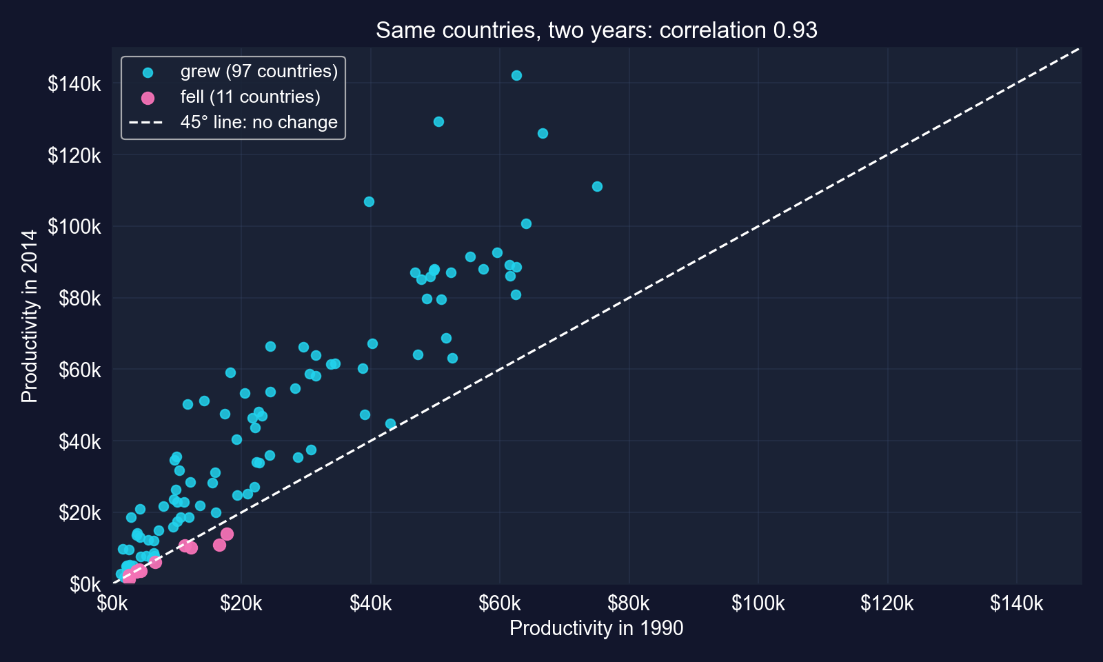
The two years are correlated 0.93: rich countries stayed rich. Differencing removes that shared level, leaving only the change.

The SD of the within-country changes ($16,920) is smaller than either year’s SD ($20,089 and $33,853) because the two years are so highly correlated. That is why the paired SE is less than half the Welch SE. Economically: the average country’s output per worker rose by about $17,800. Correlation computed for these slides.

Task 3 code: Africa versus Europe in 2014

# continues from the previous block
df_2014 = df.loc[df.index.get_level_values("year") == 2014]       # 2014 cross-section
lp_africa = df_2014.loc[df_2014["region"] == "Africa", "lp"]      # 26 countries
lp_europe = df_2014.loc[df_2014["region"] == "Europe", "lp"]      # 30 countries
t_stat, p_val = stats.ttest_ind(lp_africa, lp_europe, equal_var=False)   # Welch test
v_a, v_e = lp_africa.var() / len(lp_africa), lp_europe.var() / len(lp_europe)   # s^2/n
diff = lp_africa.mean() - lp_europe.mean()  # difference in means
se_diff = np.sqrt(v_a + v_e)                # SE of the difference
df_w = (v_a + v_e)**2 / (v_a**2 / (len(lp_africa) - 1) + v_e**2 / (len(lp_europe) - 1))  # Welch df
t_c = stats.t.ppf(0.975, df_w)              # critical value at the Welch df
print(f"diff {diff:,.0f}, t {t_stat:.2f}, p {p_val:.1e}")              # gap and test
print(f"95% CI [{diff - t_c*se_diff:,.0f}, {diff + t_c*se_diff:,.0f}]")   # CI for the gap

↗ Try it in Colab

The chapter’s Task 3 structure with “YOUR CODE HERE” completed. Welch (equal_var=False) is used, consistent with Task 2, because Europe’s SD is twice Africa’s. The pooled-variance version gives t = −11.02; the conclusion is the same.

Task 3 output: a $61,000 gap, estimated precisely

	Africa	Europe
\(n\)	26	30
Mean	$11,211	$72,572
Median	$5,722	$66,862
Std. dev.	$12,261	$25,966

Africa − Europe	Value
Difference	−$61,361
SE (Welch, df 42.6)	$5,316
\(t\)	−11.54
95% CI	[−$72,084, −$50,638]

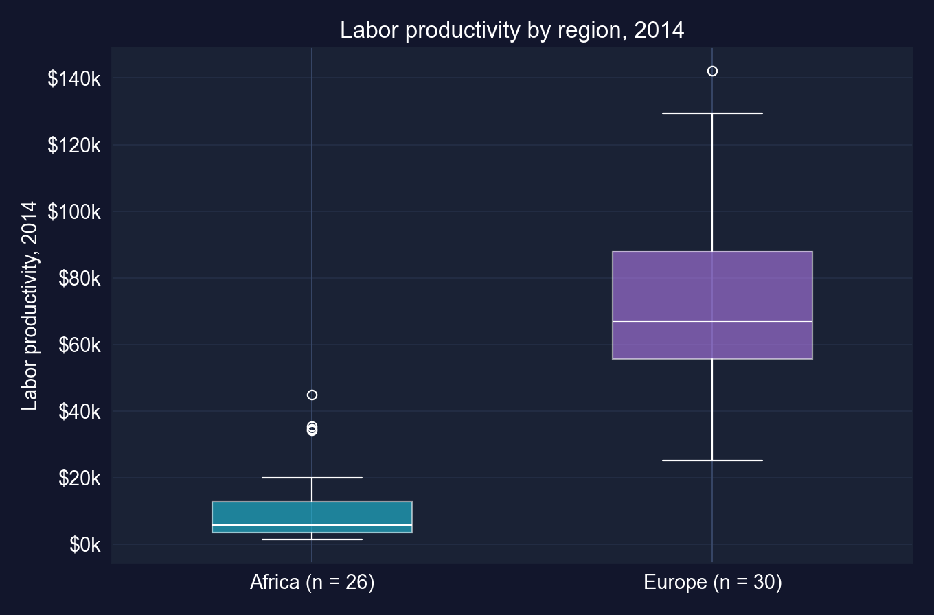
Reject equal means (\(p < 10^{-13}\)). The average European worker produces 6.5 times as much as the average African worker.

Computed for these slides. Is it real? Overwhelmingly. Does it matter? Enormously: the gap is larger than the mean of either Africa or the world. Could we tell? Easily: with an SE of $5,316 and a critical value of 2.02, any gap beyond about $10,700 would already be significant. Caveat: Africa’s distribution is very skewed (median $5,722 vs mean $11,211), with a few outliers above $30,000; the mean is not the typical African country.

Task 4 code: does the 2014 mean exceed $50,000?

# continues from the previous block
res_greater = stats.ttest_1samp(lp_2014, popmean=50000, alternative="greater")   # Ha: mu > 50,000
res_two = stats.ttest_1samp(lp_2014, popmean=50000, alternative="two-sided")     # Ha: mu != 50,000
res_less = stats.ttest_1samp(lp_2014, popmean=50000, alternative="less")         # for contrast only
print(f"mean {lp_2014.mean():,.0f}, t {res_greater.statistic:.3f}")              # t is negative
print(f"p (greater) {res_greater.pvalue:.4f}, p (two-sided) {res_two.pvalue:.4f}")  # chapter's
print(f"p (less) {res_less.pvalue:.4f}")    # never switch to this after seeing t

↗ Try it in Colab

The chapter’s Task 4 outline, written out. scipy’s ttest_1samp takes an alternative argument: “greater”, “less” or “two-sided”. The “less” line is added only to make the p-hacking point on the next slide.

Task 4 output: when the estimate points the wrong way

\(H_a\)	\(t\)	\(p\)-value	Decision at 5%
\(\mu > 50{,}000\) (the chapter’s claim)	−2.770	0.9967	do not reject
\(\mu \neq 50{,}000\)	−2.770	0.0066	reject
\(\mu < 50{,}000\) (not pre-specified)	−2.770	0.0033	—

Sample mean $40,977 · one-sided critical value 1.659 · computed for these slides

• The mean is below $50,000, so \(t < 0\) and the upper-tail \(p\) is \(1 - 0.0066/2 = 0.9967\), not half the two-sided \(p\)
• We cannot conclude productivity exceeds the benchmark; the two-sided test says it differs, on the low side
• Switching to \(H_a: \mu < 50{,}000\) after seeing the sign would be \(p\)-hacking

A one-sided \(p\)-value above 0.5 means the data point against the direction you hoped for.

This answers the chapter’s discussion question: here the one-sided p-value is larger than the two-sided one because the estimate falls on the side opposite to Ha. Type I error in this context: if the true mean were at or below $50,000, a 5% test would wrongly declare it above the benchmark at most 5% of the time.

Task 5 code: what share of countries grew?

# continues from the previous block
growth = (lp_2014.droplevel("year") > lp_1990.droplevel("year")).astype(int)   # 1 if lp rose
n = len(growth)                             # 108 countries
p_hat = growth.mean()                       # share of growth winners
se_p = np.sqrt(p_hat * (1 - p_hat) / n)     # SE at p-hat (for the CI)
ci = (p_hat - 1.96 * se_p, p_hat + 1.96 * se_p)       # 95% normal CI
z = (p_hat - 0.5) / np.sqrt(0.5 * 0.5 / n)  # z test of H0: p = 0.5
p_val = 2 * stats.norm.sf(abs(z))           # two-sided p-value
print(f"{growth.sum()} of {n}: p_hat {p_hat:.3f}, CI [{ci[0]:.3f}, {ci[1]:.3f}]")   # share
print(f"z {z:.2f}, p {p_val:.1e}")          # test of H0: p = 0.5

↗ Try it in Colab

Built from the chapter’s four hints. The droplevel step is the one the chapter’s hint warns about: comparing the raw Series fails because their (country, year) indexes differ.

Task 5 output: nine in ten countries grew

	Value
Countries with higher productivity in 2014	97 of 108
\(\hat{p}\)	0.898
95% CI	[0.841, 0.955]
\(z\) (vs 0.5)	8.28
\(p\)-value	< 10⁻¹⁵

Computed for these slides · \(n(1-\hat{p}) = 11\), just above the rule-of-thumb 10

The 11 countries where productivity fell: Cameroon, Central African Republic, Democratic Republic of Congo, Haiti, Honduras, Kyrgyz Republic, Nicaragua, Niger, Sierra Leone, Tajikistan, Togo.

Far more than half of countries grew, but all 11 that fell were in the poorer half in 1990: growth was not shared by everyone.

The fallers are concentrated in Sub-Saharan Africa, Central America and Central Asia; in 1990 all 11 ranked in the poorer half (6 of them in the poorest quarter), computed for these slides. With only 11 “failures” the normal approximation is borderline; the conclusion is far from the cutoff anyway. Caveat: the 108 countries are not a random sample of a larger population, so “inference” here is about a hypothetical super-population of countries that could have occurred.

Task 6 code: every region, every pair

# continues from the previous block (df_2014 from Task 3)
import itertools                            # all pairs of regions
by_region = df_2014.groupby("region")["lp"]                         # 5 regions
stats_r = by_region.agg(["count", "mean", "std"])                   # n, mean, s
stats_r["se"] = stats_r["std"] / np.sqrt(stats_r["count"])          # SE of each mean
stats_r["tc"] = stats.t.ppf(0.975, stats_r["count"] - 1)            # t critical, df = n - 1
for a, b in itertools.combinations(sorted(stats_r.index), 2):        # 10 pairs
    xa = df_2014.loc[df_2014["region"] == a, "lp"]                  # region a
    xb = df_2014.loc[df_2014["region"] == b, "lp"]                  # region b
    print(a, b, stats.ttest_ind(xa, xb, equal_var=False))           # Welch test
stats_r["lo"] = stats_r["mean"] - stats_r["tc"] * stats_r["se"]    # lower 95% bound
stats_r["hi"] = stats_r["mean"] + stats_r["tc"] * stats_r["se"]    # upper 95% bound
print(stats_r.round(0))                     # the CI table

↗ Try it in Colab

The chapter’s Task 6 suggested approach, implemented with a loop over itertools.combinations. With 5 regions there are 10 pairs.

Task 6 output: regional means and their CIs

Region	\(n\)	Mean	Std. error	95% CI
Africa	26	$11,211	$2,405	[$6,259, $16,164]
Americas	22	$32,836	$5,167	[$22,092, $43,581]
Asia	28	$38,725	$6,282	[$25,836, $51,615]
Europe	30	$72,572	$4,741	[$62,876, $82,268]
Oceania	2	$75,067	$10,980	[−$64,444, $214,577]

Oceania = Australia and New Zealand; with 1 degree of freedom, \(t_{1,\,0.025} = 12.7\) · computed for these slides

Four regions are estimated with useful precision; Oceania, with two countries, is not.

The chapter’s task text mentions Africa, Europe, Asia and Americas; the data also contain Oceania with only two countries. A t interval with 1 degree of freedom uses a critical value of 12.7, which is why it explodes.

Regional CIs at a glance: Oceania’s interval is useless

Mean labor productivity by region in 2014 with 95% CIs (the error-bar plot the chapter’s Task 6 asks for).

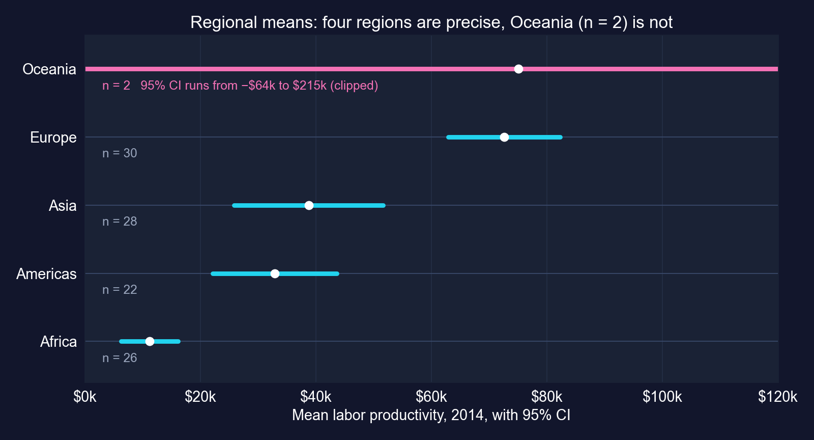
With two countries, Oceania’s interval even includes negative productivity. Its mean is not “known” in any useful sense.

Figure computed for these slides. Europe’s interval does not overlap those of Africa, the Americas or Asia; the Americas and Asia overlap heavily, matching the pairwise tests on the next slide.

Task 6 output: ten tests and the multiple-testing problem

Pair	Difference	\(t\)	\(p\)	5%?	Bonferroni (0.005)?
Africa − Europe	−$61,361	−11.54	< 0.0001	✓	✓
Americas − Europe	−$39,736	−5.67	< 0.0001	✓	✓
Asia − Europe	−$33,847	−4.30	0.0001	✓	✓
Africa − Asia	−$27,514	−4.09	0.0002	✓	✓
Africa − Americas	−$21,625	−3.79	0.0007	✓	✓
Americas − Asia	−$5,889	−0.72	0.473
Africa − Oceania	−$63,856	−5.68	0.095
Americas − Oceania	−$42,230	−3.48	0.110
Asia − Oceania	−$36,341	−2.87	0.119
Europe − Oceania	−$2,495	−0.21	0.861

Welch tests · computed for these slides

With 10 tests at 5%, the chance of at least one false alarm is up to 40%. Here the same 5 pairs survive the Bonferroni cutoff of 0.005.

Family-wise error rate for 10 independent tests: 1 − 0.95^10 = 0.401. Bonferroni divides α by the number of tests: 0.05/10 = 0.005. Every pair involving Oceania is insignificant despite gaps of up to $64,000, because two observations give almost no information: a large, possibly important, difference that we simply cannot detect. That is the “could we tell?” question again.

Case Study 1: what the six tasks add up to

• Change over time: mean productivity rose by about $17,800 (+76%); the paired test makes this unmistakable (\(t = 10.9\))
• Regional gaps: Europe is far ahead; Africa, the Americas and Asia are significantly behind it; Americas vs Asia cannot be told apart
• Breadth: 97 of 108 countries grew; all 11 that did not were in the poorer half in 1990
• Method lessons: pair when units repeat; one-sided tests can point the wrong way; many tests inflate false alarms; tiny groups give useless intervals

The right test depends on how the data were generated: same countries twice is not two independent samples.

On convergence: these tasks show large and persistent level gaps, and that the countries that fell back all started in the poorer half. A proper convergence test (does initial productivity predict growth?) needs regression, from Chapter 5 onward.

Case Study 2 · Is Bolivia’s development equal across departments?

DS4Bolivia · 333 municipalities · 9 departments · six tasks

Case Study 2 brings the chapter’s tools to subnational development in Bolivia. The chapter’s code cells for Tasks 1–6 are run here and their outputs reported; Cohen’s d and the Welch variant in Task 5 are computed for these slides.

The question: does municipal development differ across Bolivia’s departments?

Data. DS4Bolivia (ds4bolivia_v20250523.csv): 339 municipalities; 333 have complete data on the five variables used. Outcome: the Municipal Sustainable Development Index (IMDS), 0–100.

Task	Question	Tool
1	National mean IMDS?	95% CI
2	Is the average municipality at the midpoint, 50?	two-sided one-sample test
3	Which departments differ?	CI per department, forest plot
4	Is La Paz above the national mean?	one-sided test
5	How large is the gap between top and bottom departments?	two-sample test
6	What should a policy brief say?	summary table

Same toolkit, new question: statistical significance versus policy relevance.

The chapter’s text says the dataset covers 339 municipalities, which is correct for the file; the analysis sample after dropna() on mun, dep, imds, ln_NTLpc2017 and pop2017 has 333. Department sizes range from 11 (Tarija) to 87 (La Paz).

Code: load the data and summarize IMDS

import numpy as np                          # square roots
import pandas as pd                         # tabular data
from scipy import stats                     # t distribution
import matplotlib.pyplot as plt             # forest plot
url_bol = "https://raw.githubusercontent.com/quarcs-lab/ds4bolivia/master/ds4bolivia_v20250523.csv"
bol = pd.read_csv(url_bol)                  # 339 municipalities, 350+ columns
key_vars = ["mun", "dep", "imds", "ln_NTLpc2017", "pop2017"]   # variables used here
bol_key = bol[key_vars].dropna().copy()     # complete cases: 333 municipalities
print(bol_key["imds"].describe().round(2))  # IMDS summary statistics
print(bol_key["dep"].value_counts().sort_index())   # municipalities per department

↗ Try it in Colab

Self-contained; the chapter’s loading cell. All later blocks in this case study continue from it.

Output: IMDS centres just above 50

IMDS	Value
Municipalities	333
Mean	51.16
Std. dev.	6.76
Min	35.70
Median	50.80
Max	80.20

Department	\(n\)	Department	\(n\)
La Paz	87	Chuquisaca	29
Santa Cruz	55	Beni	18
Cochabamba	47	Pando	13
Potosí	38	Tarija	11
Oruro	35

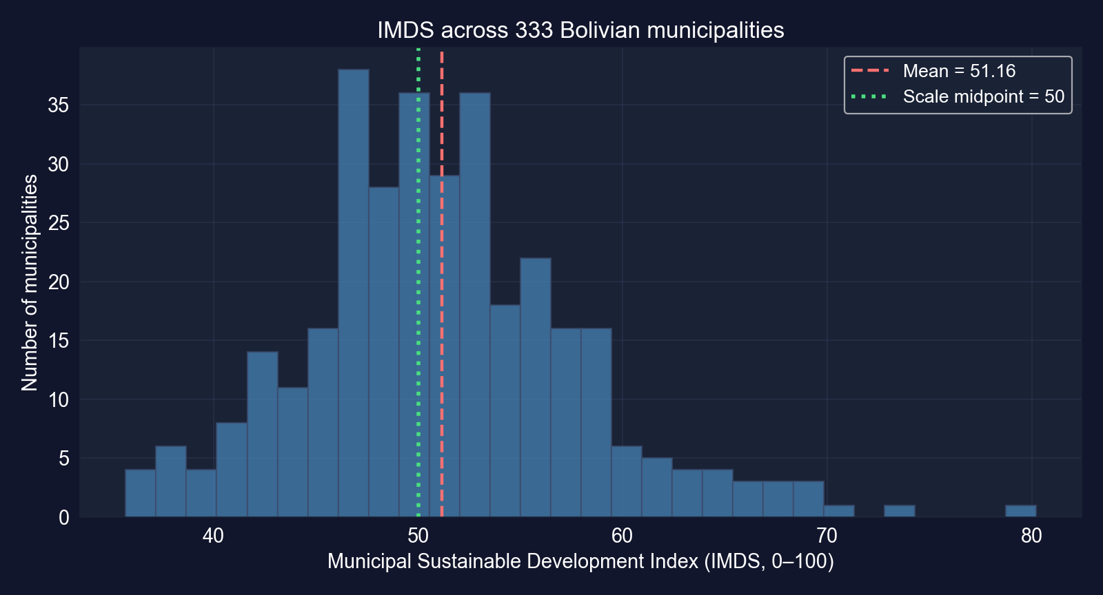
72% of municipalities score between 45 and 58. Department sizes vary eightfold, so department-level precision will vary too.

Quartiles: 47.1 and 55.0 (from the describe() output). The top score, 80.2, belongs to the municipality of La Paz (the city); the next are Cochabamba (73.7) and Tarija (70.6). Share between 45 and 58 computed for these slides.

Tasks 1–2 code: national CI and the midpoint test

# continues from the previous block
n = len(bol_key["imds"])                    # 333 municipalities
x_bar = bol_key["imds"].mean()              # national mean IMDS
se = bol_key["imds"].std() / np.sqrt(n)     # standard error
ci_low, ci_high = stats.t.interval(0.95, df=n - 1, loc=x_bar, scale=se)   # Task 1: 95% CI
t_stat, p_value = stats.ttest_1samp(bol_key["imds"], popmean=50)          # Task 2: H0: mu = 50
print(f"mean {x_bar:.4f}, se {se:.4f}, CI [{ci_low:.4f}, {ci_high:.4f}]")
print(f"t {t_stat:.4f}, p {p_value:.6f}")   # reject H0 if p < 0.05

↗ Try it in Colab

The chapter’s Task 1 and Task 2 cells combined. stats.t.interval builds x̄ ± t × se directly; ttest_1samp computes the same t statistic as section 4.4.

Tasks 1–2 output: significantly above 50, by about one point

Task	Result
1 · Mean IMDS	51.1580 (SE 0.3704)
1 · 95% CI	[50.43, 51.89]
2 · \(H_0: \mu = 50\)	\(t\) = 3.1258, \(p\) = 0.0019 → reject
2 · Gap from 50	1.16 points on a 0–100 scale

• Real? Yes: 50 lies outside the 95% CI, \(t = 3.13\)
• Does it matter? Barely: the average municipality is 1.2 points above the midpoint
• Could we tell? Easily: 333 municipalities give an SE of 0.37, so even a one-point gap stands out

Key Concept 4.12 in action: a large sample makes a small, policy-irrelevant gap statistically significant.

The chapter’s interpretation: we are 95% confident that the true mean municipal development index lies between 50.43 and 51.89. Caveat: the 333 municipalities are essentially the whole population of Bolivian municipalities, not a random sample; the “population” here is a conceptual one (the process generating municipal outcomes). Also, 50 is a scale midpoint, not a policy target, so rejecting it has limited meaning.

Task 3 code: a CI for each department

# continues from the previous block
dept_stats = (bol_key.groupby("dep")["imds"]                  # one row per department
              .agg(["mean", "std", "count"]).sort_values("mean"))   # mean, s, n
dept_stats["se"] = dept_stats["std"] / np.sqrt(dept_stats["count"])          # SE per department
dept_stats["t_crit"] = stats.t.ppf(0.975, df=dept_stats["count"] - 1)        # df = n - 1 each
dept_stats["ci_low"] = dept_stats["mean"] - dept_stats["t_crit"] * dept_stats["se"]    # lower
dept_stats["ci_high"] = dept_stats["mean"] + dept_stats["t_crit"] * dept_stats["se"]   # upper
print(dept_stats[["mean", "se", "ci_low", "ci_high", "count"]].round(2))     # the table

↗ Try it in Colab

The chapter’s Task 3 cell (its forest-plot code is shown as a figure on the next slide). Each department gets its own critical value because the degrees of freedom differ: t(10) = 2.23 for Tarija, t(86) = 1.99 for La Paz.

Task 3 output: two departments above, three below the national mean

Department	\(n\)	Mean	95% CI
Tarija	11	60.60	[56.91, 64.29]
Santa Cruz	55	54.31	[53.01, 55.62]
Cochabamba	47	52.50	[50.01, 55.00]
La Paz	87	50.98	[49.83, 52.12]
Beni	18	50.79	[48.59, 52.98]
Oruro	35	50.68	[48.96, 52.41]
Chuquisaca	29	47.80	[45.28, 50.31]
Potosí	38	47.57	[45.05, 50.09]
Pando	13	45.92	[42.39, 49.46]

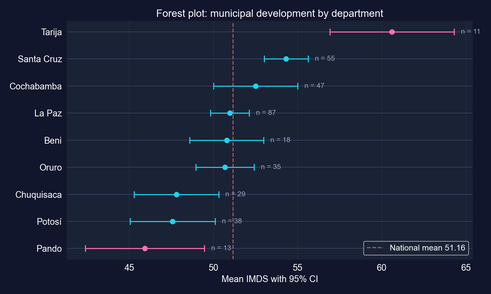
Tarija and Santa Cruz sit clearly above the national mean of 51.16; Chuquisaca, Potosí and Pando sit clearly below it.

Reading a forest plot: non-overlapping intervals imply a significant difference, but overlapping intervals do NOT imply no difference (two 95% CIs can overlap a little while the two-sample test still rejects). Use the forest plot to spot candidates, then test the comparison you care about. Small departments (Tarija 11, Pando 13) have the widest intervals: Key Concept 4.13.

Task 4 code: is La Paz above the national mean?

# continues from the previous block
la_paz = bol_key[bol_key["dep"] == "La Paz"]["imds"]   # 87 municipalities
national_mean = bol_key["imds"].mean()      # 51.16, treated as a fixed benchmark
t_stat_lp, p_two = stats.ttest_1samp(la_paz, popmean=national_mean)   # two-sided first
p_one = p_two / 2 if t_stat_lp > 0 else 1 - p_two / 2   # one-sided, Ha: mu_LP > national
print(f"La Paz mean {la_paz.mean():.4f}, t {t_stat_lp:.4f}, one-sided p {p_one:.4f}")

↗ Try it in Colab

The chapter’s Task 4 cell. The line computing p_one implements the direction check from section 4.6: halve the two-sided p only when t points the way Ha predicts.

Task 4 output: the capital department is not above average

	Value
La Paz municipalities	87
La Paz mean IMDS	50.98
National mean (benchmark)	51.16
\(t\)	−0.312
One-sided \(p\) (\(H_a\): above)	0.622
Two-sided \(p\)	0.756

• La Paz’s mean is slightly below the national mean, so the one-sided \(p\) exceeds 0.5: no evidence La Paz is more developed
• Caveat: the benchmark includes La Paz itself (87 of 333 municipalities, 26%) and is treated as a known constant; a two-sample comparison of La Paz versus the rest would be cleaner

Housing the seat of government does not make the department’s municipalities more developed on average.

Most of La Paz’s 87 municipalities are rural; the cities of La Paz and El Alto count as just two of them. A department mean weights every municipality equally, regardless of population, so it describes the typical municipality, not the typical person.

Task 5 code: the top department versus the bottom one

# continues from the previous block
dept_means = bol_key.groupby("dep")["imds"].mean()   # mean IMDS by department
top_dept, bot_dept = dept_means.idxmax(), dept_means.idxmin()   # Tarija and Pando
top_values = bol_key[bol_key["dep"] == top_dept]["imds"]         # 11 municipalities
bot_values = bol_key[bol_key["dep"] == bot_dept]["imds"]         # 13 municipalities
t_stat_2s, p_value_2s = stats.ttest_ind(top_values, bot_values)  # pooled-variance test (chapter)
t_w, p_w = stats.ttest_ind(top_values, bot_values, equal_var=False)   # Welch, for comparison
n1, n2 = len(top_values), len(bot_values)   # group sizes
pooled_var = ((n1 - 1) * top_values.var() + (n2 - 1) * bot_values.var()) / (n1 + n2 - 2)
sp = np.sqrt(pooled_var)                    # pooled standard deviation
gap = top_values.mean() - bot_values.mean() # the development gap
print(f"gap {gap:.2f}, t {t_stat_2s:.3f}, p {p_value_2s:.1e}")   # chapter's test
print(f"Welch t {t_w:.3f}, p {p_w:.1e}, Cohen's d {gap / sp:.2f}")   # added checks

↗ Try it in Colab

The chapter’s Task 5 cell uses stats.ttest_ind with its default equal_var=True (pooled variance). The Welch version and Cohen’s d (the gap in pooled-SD units, suggested in the chapter’s Task 6 cell) are computed for these slides.

Task 5 output: a 14.7-point gap between Tarija and Pando

	Tarija (top)	Pando (bottom)
Municipalities	11	13
Mean IMDS	60.60	45.92
Std. dev.	5.50	5.85

Comparison	Value
Gap	14.68 points
\(t\) (pooled) / \(p\)	6.292 / 0.0000025
\(t\) (Welch) / \(p\)	6.326 / 0.0000024
Cohen’s \(d\)	2.58 SDs

Welch and Cohen’s \(d\) computed for these slides

Real and large: the gap is about 2.6 within-department standard deviations, more than twice the national SD of IMDS.

The chapter’s code labels gaps above 10 points as “substantial”: a rule of thumb, not a statistical criterion. Caveat: the two departments were picked because they are the extremes among 9 departments (36 possible pairs). Picking the largest gap after looking inflates its significance; here the gap is so large that the conclusion survives any reasonable correction, but the habit matters.

Task 6: what the policy brief should say

• Differences are real: Tarija (60.6) and Santa Cruz (54.3) lead; Pando (45.9), Potosí (47.6) and Chuquisaca (47.8) lag, with CIs excluding the national mean of 51.2
• Some are not policy-relevant: the national mean is significantly above 50, but by only 1.2 points
• Precision is uneven: Tarija and Pando rest on 11 and 13 municipalities; their CIs are about 7 points wide
• Limits: municipalities are not people (no population weights); the 333 are nearly the whole country; IMDS is a composite index; 36 possible department pairs invite false alarms

A good brief reports the gap, its CI and its policy meaning, and says what the test cannot tell us.

The chapter’s Task 6 asks for a 200–300 word brief; its code cell builds the department summary table shown on the Task 3 slide. Tarija’s CI is 7.4 points wide and Pando’s 7.1. Key Concepts 4.12 and 4.13 both apply.

Reading it right

Act III · The resolution

Synthesis: put every test on one ruler, revisit the thread (real? matters? could we tell?), choose the right test, and leave with a checklist.

Every test in the deck on one ruler

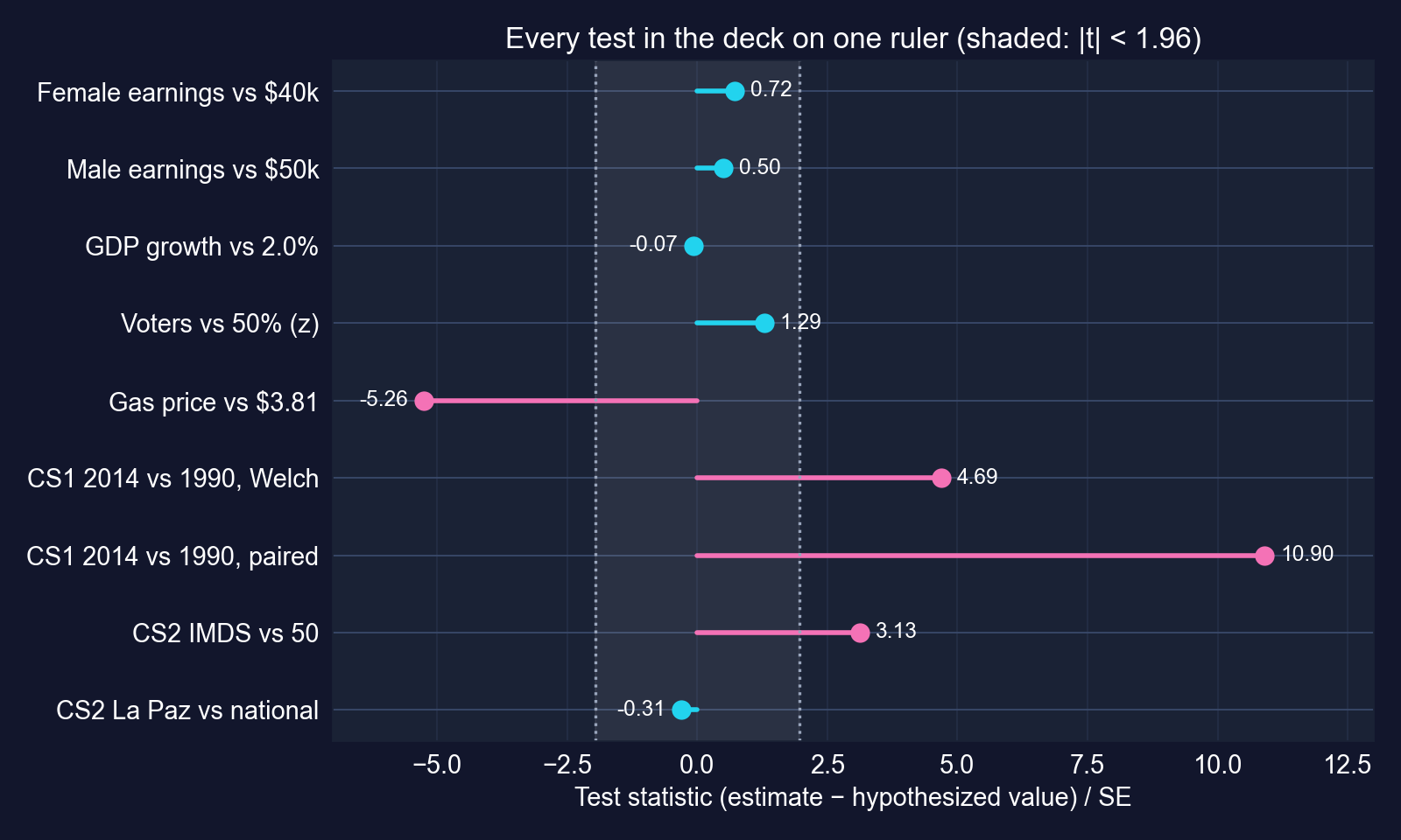
Test statistics from sections 4.4–4.7 and both case studies. Inside the shaded band, \(\lvert t \rvert < 1.96\): no rejection at 5%.

The same ±1.96 band decides every verdict. What changes is what the gap means.

All numbers are from the slides above. Note the two bars for Case Study 1, Task 2: the same mean change gives t = 4.69 when the two years are wrongly treated as independent samples and t = 10.90 when they are correctly paired.

The thread, case by case: real? matters? could we tell?

Test	Real?	Matters?	Could we tell?
Gas vs $3.81	yes, \(t = -5.26\)	yes, ≈ $109/year	yes: tiny SE
Female earnings vs $40k	no, \(t = 0.72\)	possibly	no: power 0.11 at $41,413
Male earnings vs $50k	no, \(t = 0.50\)	possibly	no: SE $4,706 from heavy tails
GDP growth vs 2%	no, \(t = -0.07\)	yes, 1 pp compounds	less than it looks: autocorrelation 0.87
Poll vs 50%	no, \(z = 1.29\)	yes, elections are close	not at \(n = 921\); just at 2,500
CS1 2014 vs 1990	yes, paired \(t = 10.9\)	yes, +$17,753	yes, once paired
CS2 IMDS vs 50	yes, \(t = 3.13\)	barely: 1.2 points	yes: \(n = 333\)
CS2 Tarija vs Pando	yes, \(t = 6.29\)	yes, 14.7 points	yes, despite \(n\) = 11, 13

Significance answers only the first column. A complete answer fills in all three.

The recurring thread of the deck in one table. Note the two “no” rows in the third column: when we cannot tell, a non-rejection is uninformative, and the confidence interval is the honest summary.

Choosing the right test

Situation	Test	Python	Example
One mean vs a value	one-sample \(t\)	stats.ttest_1samp	earnings vs $40,000
Directional claim, fixed in advance	one-sided \(t\)	alternative="greater"	La Paz vs national mean
Two independent groups	Welch two-sample \(t\)	stats.ttest_ind(…, equal_var=False)	Africa vs Europe
Same units measured twice	paired \(t\)	stats.ttest_rel	1990 vs 2014, same countries
Yes/no outcome	proportion \(z\)	stats.norm	voters, growth winners
Many comparisons	adjust \(\alpha\)	Bonferroni \(\alpha/k\)	10 regional pairs
Dependent over time	HAC SEs (Ch. 12, 17)	—	GDP growth

Match the test to how the data were generated: independence, pairing, direction and the number of tests all matter.

Welch’s version is a safe default for two groups; the pooled version assumes equal variances. The last row is a pointer: the chapter’s GDP test assumes independence that the data do not have.

The tempting mistakes — and the corrections

Objection. “\(p < 0.05\), so the effect is real and important; \(p > 0.05\), so there is no effect.”

Response. Bolivia’s mean IMDS differs “significantly” from 50 by 1.2 points: real but unimportant. Female earnings were not significantly above $40,000, yet the test had an 11% chance of detecting a $1,400 gap: no rejection, but no evidence of no effect either.

Report the estimate and its confidence interval first; the \(p\)-value is a footnote to them.

The chapter’s “Common Mistakes to Avoid”: a p-value is not the probability that H0 is true; statistical significance is not practical importance; a one-sided test needs prior justification.

Five questions to ask of any test

1. What exactly is \(H_0\), and is the claim of interest in \(H_a\)? Was the direction fixed in advance?
2. Are the observations independent? Repeated units call for pairing; time series and clusters need other SEs
3. How big is the gap, in units that matter (dollars, points, percentage points)?
4. How wide is the CI, and what is the power? Could the test have detected a gap that matters?
5. How many tests were run? Ten tests at 5% raise the chance of a false alarm to about 40%

These five questions turn a \(p\)-value from a verdict into evidence.

A checklist students can apply to every inference table in the rest of the book. Questions 2 and 4 are the ones the chapter’s own GDP and earnings examples needed most.

What to carry forward

• The standard error \(s/\sqrt{n}\) drives every interval and test, and it shrinks only with \(\sqrt{n}\)
• Use the \(t\) distribution when \(\sigma\) is estimated; by \(n \approx 100\) it is close to the normal
• A 95% CI is the set of values a two-sided 5% test would not reject; read it as a repeated-sampling statement
• \(t = (\text{estimate} - \text{hypothesized value})/\text{SE}\): the recipe for every test in Chapters 7–17
• Fail to reject ≠ accept: check power and the CI before concluding “no effect”
• Real, matters, could we tell? Ask all three of every result

Recap of the chapter’s Key Takeaways, updated with what the deck verified: power, pairing, multiple testing and dependence.

Estimate the mean, bound it with a CI, then test the claim you care about, and ask whether it matters.