The question

Act I · The tension

Do bigger houses really sell for more — and by how much?

A dataset of house sales: for each house we see two numbers — its size and its price.

Eyeballing one house tells us nothing. The relationship between the two columns is the story — and we want to measure it, not just sense it.

Open with the concrete question. We have bivariate data: two measurements per observation. The whole chapter is about summarizing the link between them with a number and a line.

Where we’re going

• See the relationship — scatterplots and two-way tables
• Measure its strength — correlation and covariance
• Model it — the ordinary-least-squares (OLS) regression line
• Judge the fit — \(R^2\) and the standard error of the regression
• Interpret it honestly — association is not causation

Three ideas carry the whole chapter

Association — do \(x\) and \(y\) tend to move together, and in which direction?

Correlation \(r\) — a single, unit-free number in \([-1, 1]\) for the strength of a linear link.

Regression — a line \(\hat{y} = b_1 + b_2 x\) that predicts \(y\) from \(x\).

Summarizing a relationship means turning a cloud of points into a direction, a number, and a line.

These three terms recur in every later chapter. Correlation measures; regression predicts.

Seeing and measuring the link

Act II · The investigation

Start by looking: price rises with size — but not perfectly

Each dot is a house. The upward drift is the association; the scatter around it is everything size doesn’t explain.

A scatterplot is the first summary of bivariate data — direction and spread, before any number.

Point out the clear positive slope and the vertical spread at any given size — other factors (lot, age, location) move price too.

Draw the scatterplot in a few lines

import pandas as pd                          # tabular data
import matplotlib.pyplot as plt               # plotting

url = "https://raw.githubusercontent.com/quarcs-lab/data-open/master/AED/AED_HOUSE.DTA"
houses = pd.read_stata(url)                  # load the 29 Davis, CA house sales

fig, ax = plt.subplots(figsize=(10, 6))      # create one figure + axes
ax.scatter(houses["size"], houses["price"],  # x = size, y = price
           s=80, alpha=0.7, color="#22d3ee") # marker size, transparency, colour
plt.show()                                   # render the scatter plot

↗ Try it in Colab

matplotlib is the workhorse plotting library. One scatter call turns the two columns into the picture on the previous slide.

Correlation measures strength; covariance only gives the sign

Covariance

• sign tells the direction
• carries the units of \(x \times y\) (dollars × sq ft)
• scale is not comparable across datasets

Correlation \(r\)

• unit-free, always in \([-1, 1]\)
• \(r = s_{xy} / (s_x s_y)\)
• comparable across any pair of variables

Covariance says which way; correlation says how strongly — on a scale anyone can read.

\(r\) captures linear strength — and can miss a curve

Same idea, four strengths: strong, moderate, none, and negative. Correlation ranks the first three by how tightly points hug a line.

\(r\) near \(\pm 1\) means a tight line; \(r \approx 0\) means no linear link — not necessarily no link at all.

Zero correlation can still hide a strong non-linear relationship (e.g. a U-shape). r only sees the straight-line part. For our house data r = 0.7858.

Measure the link: correlation and covariance in pandas

import pandas as pd                          # tabular data

url = "https://raw.githubusercontent.com/quarcs-lab/data-open/master/AED/AED_HOUSE.DTA"
houses = pd.read_stata(url)                  # load the 29 Davis, CA house sales

cov = houses[["price", "size"]].cov()        # covariance matrix (carries units: $ × sq ft)
corr = houses[["price", "size"]].corr()      # correlation matrix (unit-free, in −1…1)

r = corr.loc["price", "size"]                # pull out the single correlation number
print(f"r = {r:.4f}")                        # → r = 0.7858

↗ Try it in Colab

.corr() and .cov() are pandas DataFrame methods. The off-diagonal cell is the number we want; correlation standardizes covariance by the two standard deviations.

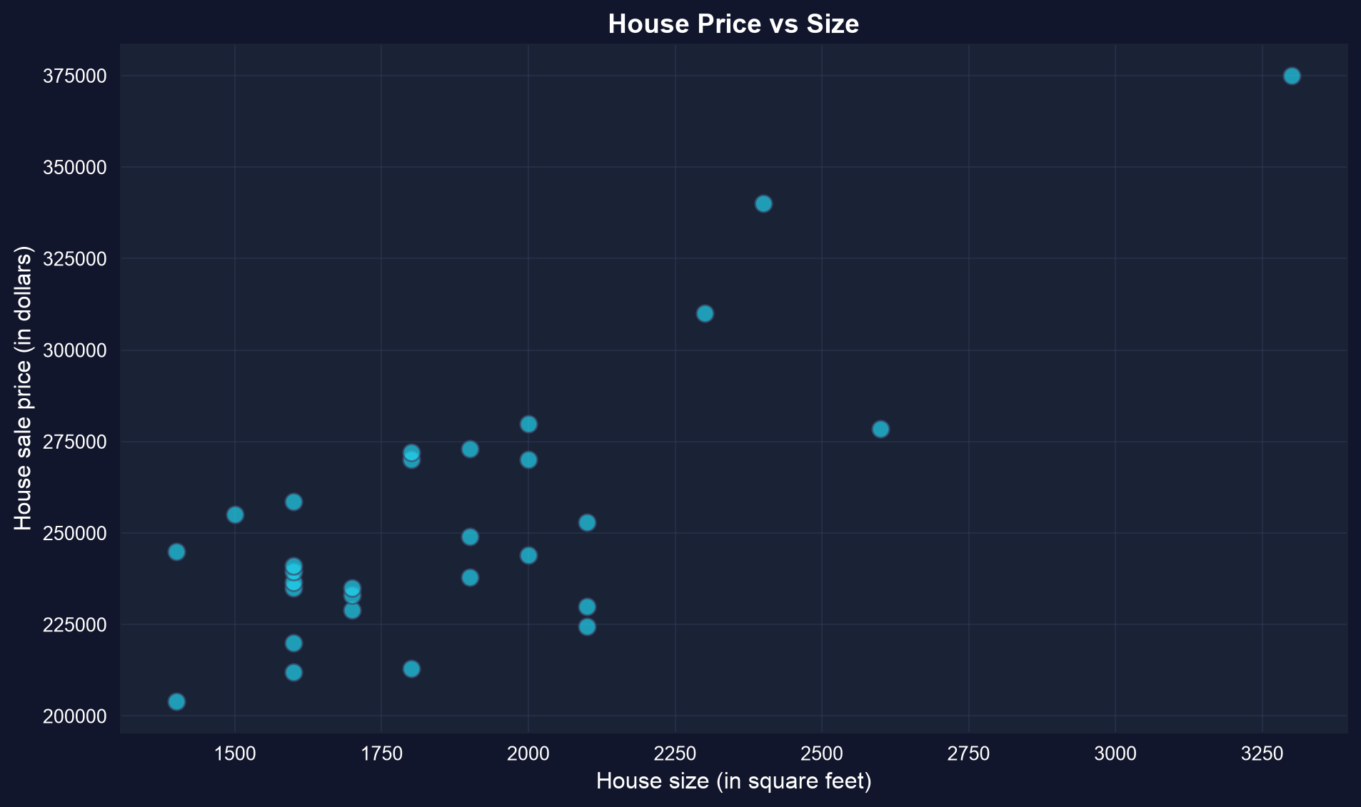
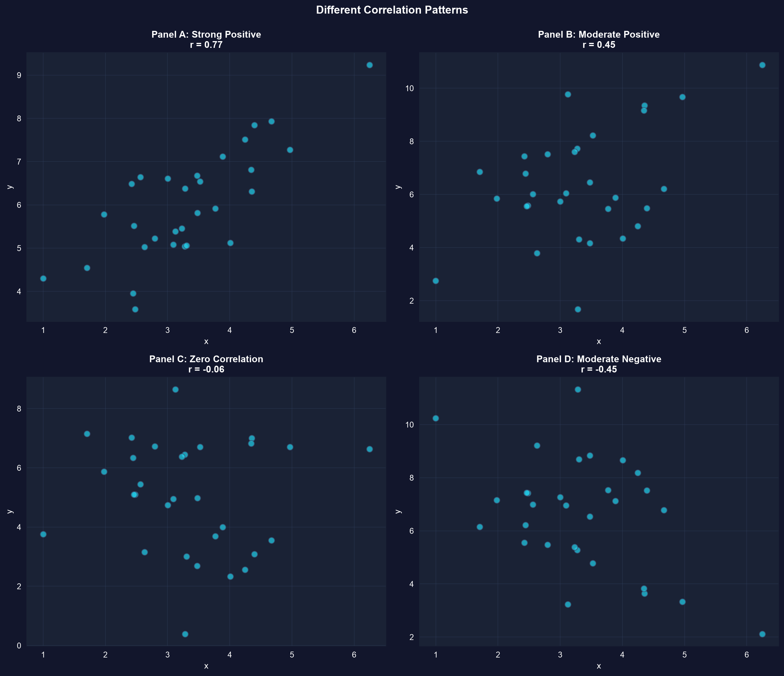
The regression line turns the cloud into a prediction

\[\hat{y} = b_1 + b_2\, x\]

\(b_1\) is the intercept (predicted \(y\) when \(x = 0\)); \(b_2\) is the slope — the predicted change in \(y\) for a one-unit increase in \(x\). OLS picks \(b_1, b_2\) to minimize the sum of squared residuals.

Define residual e_i = y_i − ŷ_i. OLS minimizes Σ e_i². This generalizes the sample mean: an intercept-only regression returns ȳ.

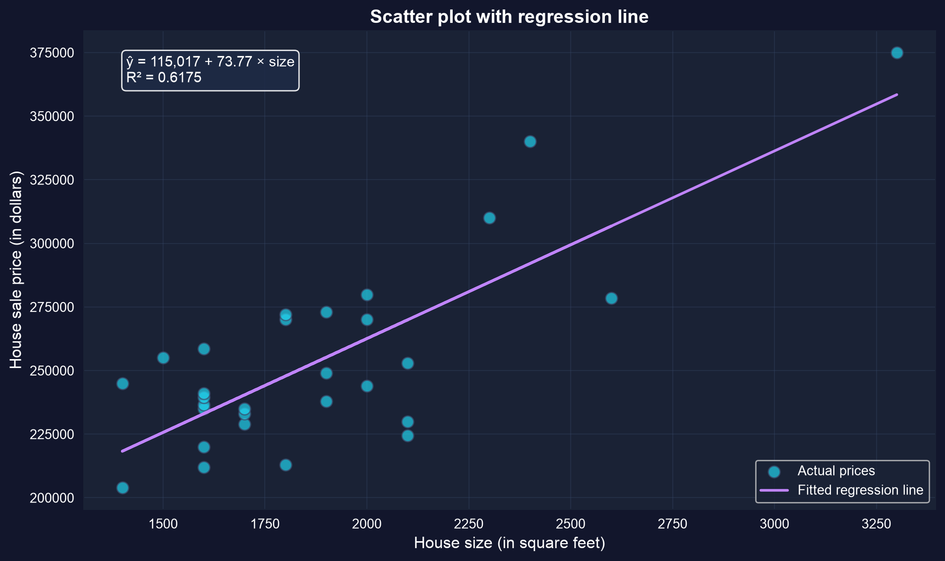
OLS draws the single best-fitting line through the cloud

The fitted line: ŷ = 115,017 + 73.77 × size. Each extra square foot predicts about $74 more.

Slope \(b_2 = \$73.77\) per sq ft; intercept \(b_1 = \$115{,}017\) — a house 100 sq ft larger is predicted to cost about $7,377 more.

The slope is the economically meaningful number. The intercept here is an out-of-range extrapolation (no 0-sq-ft houses), so don’t over-interpret it.

Fit the regression line in Python

!pip install -q pyfixest                   # install pyfixest in Colab (-q = quiet; not preinstalled)

import pandas as pd                         # pandas → load & handle tabular data
import pyfixest as pf                        # pyfixest → fast OLS regression + tidy output

# dataset: 29 house sales in Davis, CA (price, size, bedrooms, …)
url = "https://raw.githubusercontent.com/quarcs-lab/data-open/master/AED/AED_HOUSE.DTA"
houses = pd.read_stata(url)                 # read the Stata .dta file into a DataFrame

m = pf.feols("price ~ size", data=houses)   # fit OLS: regress price on size
m.summary()                                 # report intercept b1, slope b2, SEs, R²

↗ Try it in Colab

Self-contained — paste it into an empty Colab cell and it runs end to end: load the AED house data straight from the project’s open-data repo, then fit and report the regression. pyfixest is the project’s estimation package. (The deck itself doesn’t execute; this is the runnable workflow.)

\(R^2\) splits total variation into explained and left-over

\[R^2 = \frac{\text{explained SS}}{\text{total SS}} = 1 - \frac{\text{residual SS}}{\text{total SS}}\]

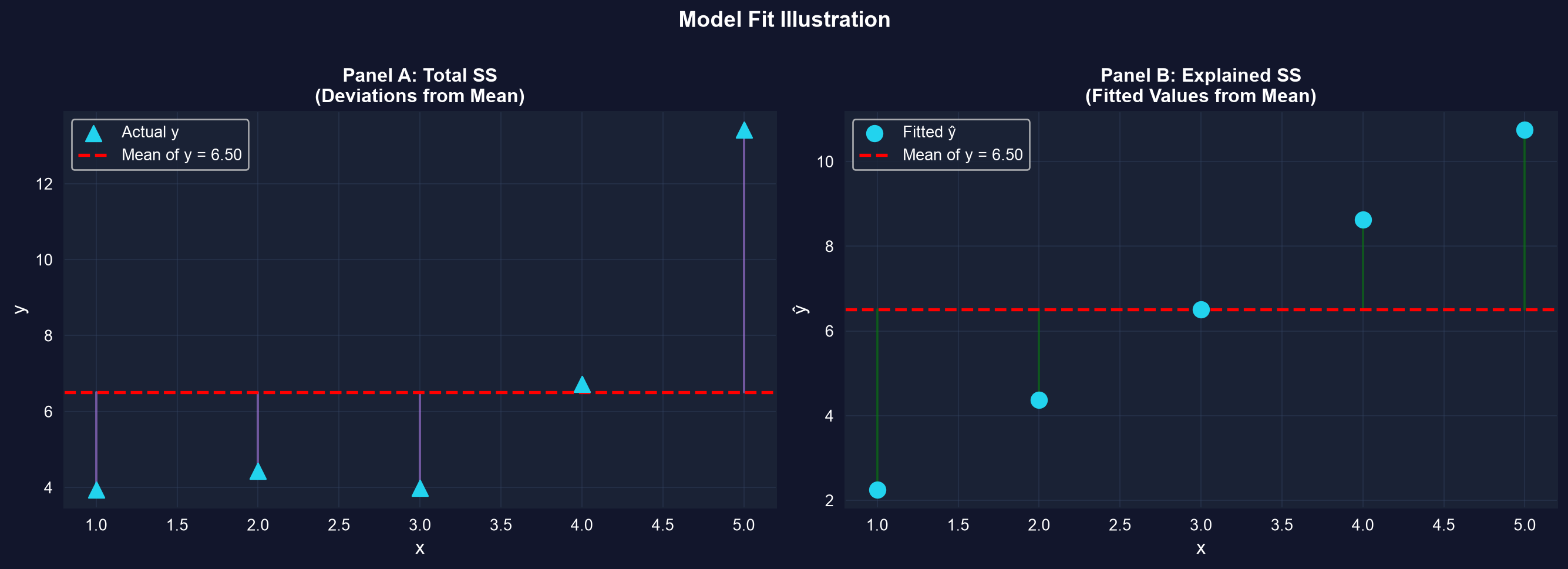
Total variation in price = what the line explains + what it leaves in the residuals.

Here \(R^2 = 0.617\): size explains about 62% of the variation in price, leaving 38% to everything else. (And \(R^2 = r^2 = 0.7858^2\).)

For simple regression R² always equals r². The standard error of the regression, s_e, measures the typical residual in the units of y (dollars).

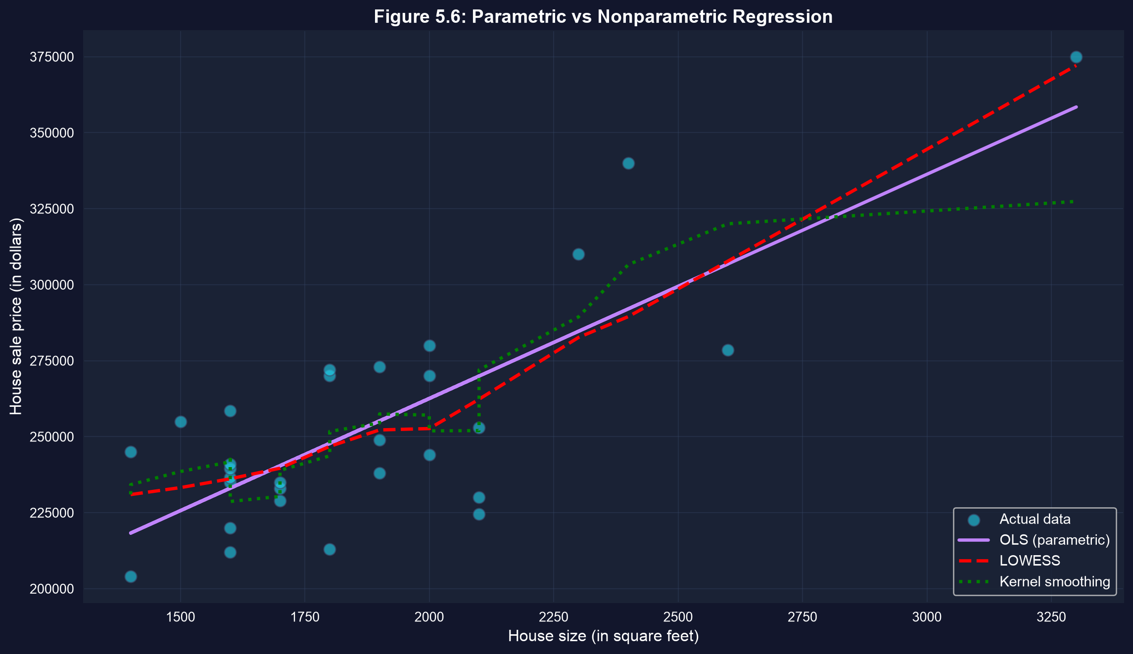
A flexible curve checks the straight-line assumption

Nonparametric regression lets the data choose the shape — if it tracks the OLS line, linearity is a fair summary.

Fit a flexible curve first; if it hugs the straight line, the simple linear summary is trustworthy.

Nonparametric regression imposes no functional form. Comparing it to the OLS line is a quick, honest check that the linear model isn’t hiding curvature.

Reading it right

Act III · The resolution

The tempting mistake — and the correction

Objection. “Size and price have \(r = 0.79\), so larger size causes higher price.”

Response. Association is not causation. Confounders (location; lot size, though only weakly linked to size and price here), reverse causality, and selection can all create a correlation. A line summarizes; it does not identify a cause.

A correlation earns a causal reading only with a design that rules out the alternatives.

What to carry forward

• A scatterplot is the first, honest summary of two variables.
• Correlation \(r \in [-1, 1]\) measures linear strength, unit-free; covariance gives only the sign.
• OLS fits \(\hat{y} = b_1 + b_2 x\) by minimizing squared residuals; the slope is the headline.
• \(R^2\) reports the share of variation explained — and \(R^2 = r^2\) for simple regression.
• Association \(\neq\) causation — always the last word on interpretation.

Measure the relationship, model it with a line — then resist calling it a cause.