The question

Act I · The tension

We fit one line — but the truth lives in a population we never see

Chapter 5 showed us how to fit a regression. But our line \(\hat{y} = b_1 + b_2 x\) comes from one noisy sample. Behind it sits a population line \(\beta_1 + \beta_2 x\) we can never observe.

So why should we trust an estimate we know is wrong? This chapter answers that — with the statistical properties that make OLS the default estimator in econometrics.

The whole chapter is about the gap between the sample line we compute and the population line we want. Properties like unbiasedness tell us how to reason about that gap.

Where we’re going

• Population vs sample — the line we want (\(\beta_1+\beta_2x\)) vs the line we get (\(b_1+b_2x\))
• Sampling variability — why every sample gives a different line
• Unbiasedness — why OLS is right on average, shown by Monte Carlo
• Standard errors — how to measure the precision of a single estimate
• BLUE & normality — why OLS is the best choice, and why \(t\)-tables work

Six ideas anchor this chapter

• Conditional mean \(E[Y\mid X]\) — the population line; the systematic part of \(Y\) given \(X\)
• Error \(u\) vs residual \(e\) — the unobserved shock vs the observed miss from \(\hat{y}\)
• Homoskedasticity — the error spread \(\operatorname{Var}[u\mid x]=\sigma_u^2\) is constant in \(x\)
• \(s_e\) — the standard error of the regression, \(\sqrt{\text{RSS}/(n-2)}\): typical residual size
• BLUE — under the four assumptions, OLS has the smallest variance of any linear unbiased rule
• Asymptotic normality — as \(n\) grows, \(b_2\) is approximately normal, so \(t\)-tables apply

OLS is wrong in every sample — but right on average, and we can say exactly how wrong.

Population vs sample

Act II · The investigation

A known truth: data generated from \(y = 1 + 2x + u\)

To study OLS, the chapter uses generated data where we know the answer:

\[y = \underbrace{1 + 2x}_{E[y\mid x]} + u, \qquad u \sim N(0,\ \sigma_u^2=4)\]

True intercept \(\beta_1=1\), true slope \(\beta_2=2\). The column Eygivenx is the population line exactly; u is the random shock that pulls each observed y off it.

Step 1 — fit the sample line with pyfixest, compare to the truth

!pip install -q pyfixest                     # install pyfixest in Colab (-q = quiet; not preinstalled)

import pandas as pd                          # tabular data
import pyfixest as pf                         # pyfixest → OLS, R-style formulas

url = "https://raw.githubusercontent.com/quarcs-lab/data-open/master/AED/AED_GENERATEDDATA.DTA"
data = pd.read_stata(url)                    # 5 points generated from y = 1 + 2x + u

fit = pf.feols("y ~ x", data=data)           # OLS: regress observed y on x
fit.coef()                                   # sample estimates b1, b2
fit.summary()                                # full table: coefs, SEs, t, p, R2

↗ Try it in Colab

Fitting observed y (not Eygivenx) gives b1 = 2.81, b2 = 1.05, R2 = 0.769 — off from the true 1 and 2 because n = 5 and the errors happened to pull the line. That gap is the whole point.

One sample misses: \(\hat{y} = 2.81 + 1.05x\) vs the true \(1 + 2x\)

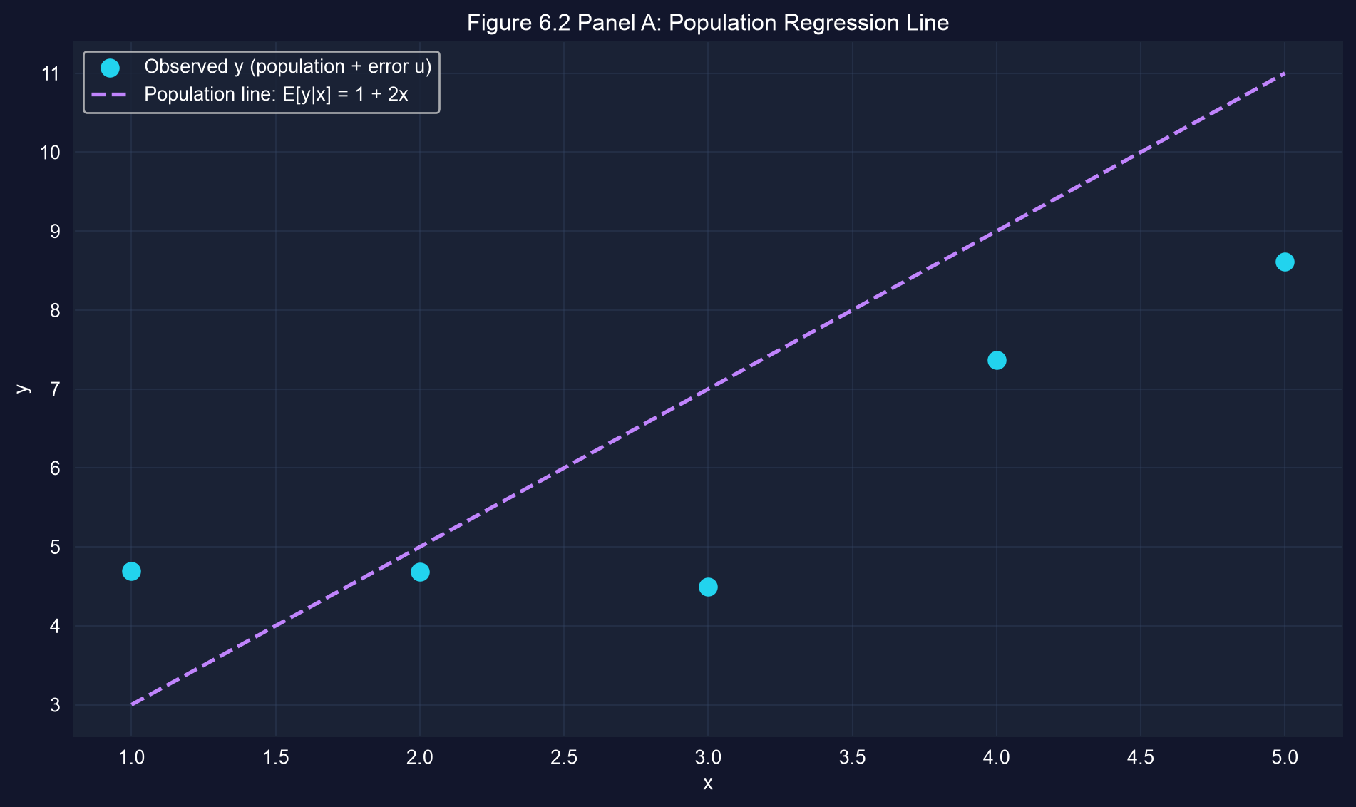
Observed points (cyan) scatter around the true population line (purple dashed). The sample line fit to them need not match it.

With only \(n=5\), the estimate (\(b_2=1.05\)) lands far from the truth (\(\beta_2=2\)). This is not a bug — it is sampling variability.

Same process, three samples, three different lines

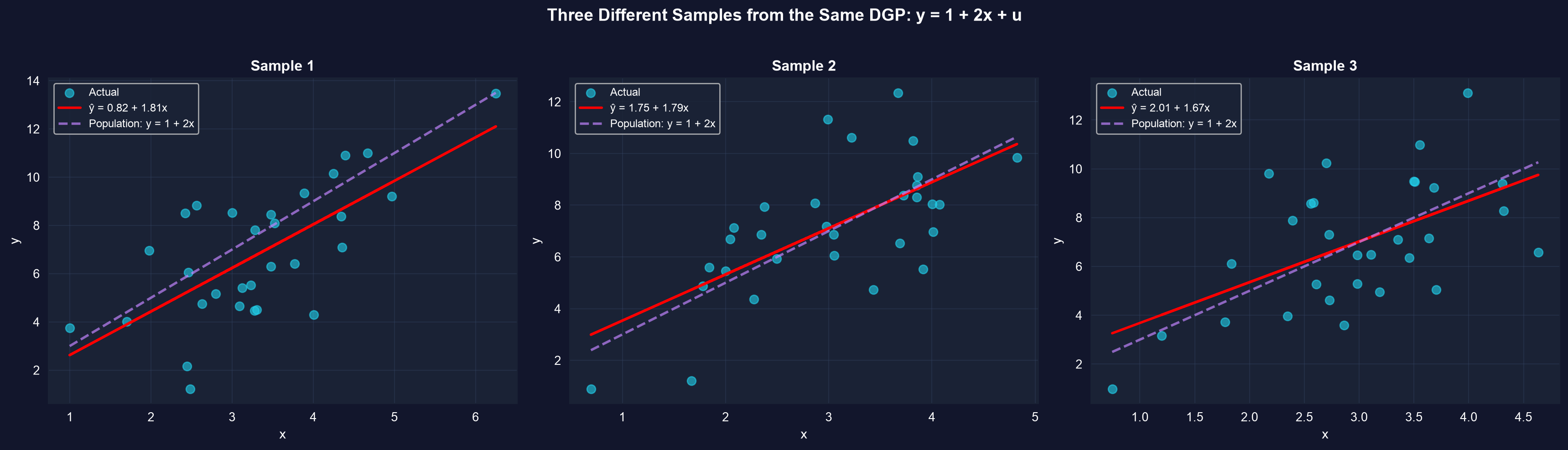
Three independent samples from the identical DGP \(y=1+2x+u\) yield three different fitted lines — all near the true population line, none on it.

Slopes came out 1.81, 1.79, 1.67; intercepts 0.82, 1.75, 2.01. One sample never reveals the truth — it only gives one draw from a distribution of estimates.

Step 2 — simulate 1,000 samples to see the estimator’s behavior

import numpy as np                           # random draws + arrays
import pyfixest as pf                         # OLS on each simulated sample

np.random.seed(42)                           # reproducible simulation
n, n_sims = 30, 1000                         # 1,000 samples of n = 30
b1_true, b2_true, sigma_u = 1, 2, 2          # the known DGP y = 1 + 2x + u

slopes = []                                  # collect b2 from each sample
for _ in range(n_sims):
    x = np.random.normal(3, 1, n)            # draw regressors
    u = np.random.normal(0, sigma_u, n)      # draw mean-zero errors
    y = b1_true + b2_true * x + u            # build y from the true model
    slopes.append(pf.feols("y ~ x", data=pd.DataFrame({"x": x, "y": y})).coef()["x"])

np.mean(slopes)                              # ≈ 2.00  → unbiased
np.std(slopes)                               # ≈ 0.38  → sampling variability

↗ Try it in Colab

Monte Carlo = repeat the study 1,000 times on the computer. Mean slope 1.9944, SD 0.3836; mean intercept 0.9960, SD 1.2069. The average lands on the truth even though no single sample does.

Right on average: the estimates center on the true \(\beta_2 = 2\)

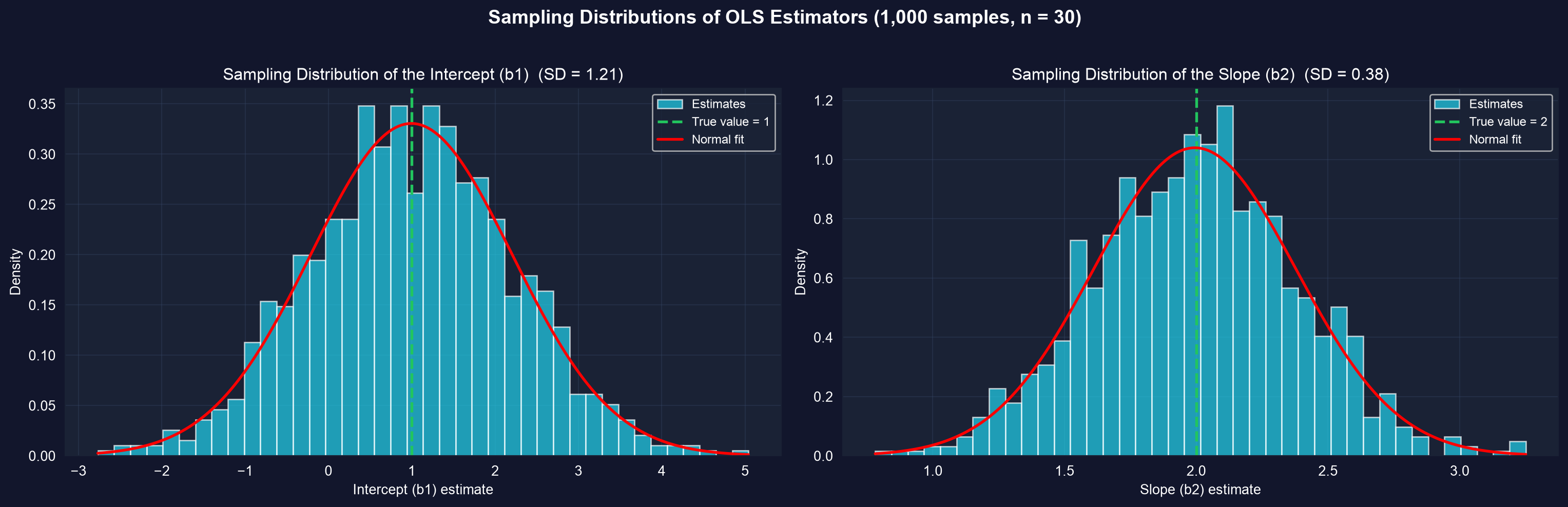
Across 1,000 samples, the slope and intercept estimates form bell curves centered on the true values, tracking a normal fit.

Mean slope \(=1.994\) (true \(2\)), SD \(=0.38\); mean intercept \(=0.996\) (true \(1\)). Unbiasedness and asymptotic normality, seen directly.

6.4 — precision has a formula: the standard error of the slope

For a single sample we can’t average over worlds — but we can estimate the spread:

\[s_e=\sqrt{\frac{\text{RSS}}{n-2}}, \qquad se(b_2)=\frac{s_e}{\sqrt{\sum_i (x_i-\bar{x})^2}}\]

Divide RSS by \(n-2\) because two parameters (\(b_1,b_2\)) are estimated. The slope is precise when \(s_e\) is small (good fit) and the \(x\)’s are widely spread.

Step 3 — compute the standard errors by hand, verify against the model

import numpy as np                           # arrays + math
import pyfixest as pf                         # to check our hand calculation

data = pd.DataFrame({"x": [1, 2, 3, 4, 5],   # artificial 5-point dataset
                     "y": [1, 2, 2, 2, 3]})
fit = pf.feols("y ~ x", data=data)           # fitted line: y_hat = 0.8 + 0.4x

b1, b2 = fit.coef()["Intercept"], fit.coef()["x"]
data["resid"] = data["y"] - (b1 + b2 * data["x"])   # residuals e = y - y_hat
RSS = np.sum(data["resid"] ** 2)             # residual sum of squares
Sxx = np.sum((data["x"] - data["x"].mean()) ** 2)   # spread of x

s_e   = np.sqrt(RSS / (len(data) - 2))       # standard error of the regression
se_b2 = s_e / np.sqrt(Sxx)                   # standard error of the slope

print(se_b2, fit.se()["x"])                  # hand value == model value ✓

↗ Try it in Colab

Standard errors aren’t magic — RSS → s_e → se(b2) from transparent formulas, and the hand number matches pyfixest’s reported SE exactly. This demystifies the regression table.

Three levers control precision

• Model fit (\(s_e\)) — smaller residuals shrink every standard error.
• Sample size (\(n\)) — \(se(b_2)\propto 1/\sqrt{n}\): quadruple \(n\) to halve the SE.
• Spread of \(x\) — a wide \(\sum(x_i-\bar{x})^2\) pins the slope down; clustered \(x\) leaves it loose.

In the 108-country convergence data, capital per worker is spread almost as wide as its mean — exactly the condition that estimates the slope precisely.

Reading it right

Act III · The resolution

“My estimate is wrong — so OLS failed.” Not quite.

Objection. “My slope is 1.05 but the truth is 2.0. The method is broken.”

Response. A single wrong estimate is expected, not a failure. Under the four assumptions (correct model, mean-zero errors, homoskedasticity, independence) OLS is unbiased — right on average — and BLUE, the tightest linear unbiased rule. One sample is one draw; the standard error tells you how far it might be off.

Don’t ask “is my estimate exactly right?” Ask “how precise is it?” — that’s what the standard error reports.

What to carry forward

• The population line \(\beta_1+\beta_2x\) is the target; the sample line \(b_1+b_2x\) is one noisy estimate of it.
• OLS is unbiased: \(E[b_2]=\beta_2\) — Monte Carlo centers 1,000 estimates on the truth.
• Standard errors quantify sampling variability; \(se(b_2)=s_e/\sqrt{\sum(x_i-\bar{x})^2}\).
• Precision improves with better fit, larger \(n\), and wider spread in \(x\).
• Under the four assumptions OLS is BLUE and asymptotically normal — the license for \(t\)-tests and intervals.

Fit the line, report its standard error — the estimate is a draw, not the truth.