One sample, one slope: how much should we trust it?

Act I · The tension

This chapter turns a regression slope into a statement about the population. Chapter 6 gave us the point estimate; Chapter 7 tells us how precise it is, which values of the true slope the data rule out, and how to test claims about it. The same toolkit then gets applied to two real case studies: 108 countries and 333 Bolivian municipalities.

A slope estimate is never the whole story

Chapter 6 gave us a number: in 29 houses sold in Davis, California, each extra square foot goes with $73.77 more in price. A different sample of 29 houses would give a different number.

So the real question is not “what is the slope?” but “how much should we trust it?” Inference turns one estimate into a range (a confidence interval) and a verdict (a hypothesis test).

Every result in this deck answers three questions: Is it precise? Is it real? Does it matter? And a fourth one underneath: is the standard error honest?

The estimate b2 = 73.77 is one draw from a sampling distribution. Inference describes that distribution using only the one sample we have. The four questions are the recurring thread of the deck: precision (SE and CI), statistical significance (tests), economic significance (magnitude in context), and honest uncertainty (classical vs heteroskedasticity-robust SEs). They come back as a scorecard at the end of each part and in the synthesis.

Where we are going: click any part to jump to it

Part	Question	Tool	Headline result
7.1	Do bigger houses sell for more?	OLS, 29 houses	\(b_2 = 73.77\) $/sq ft
7.2	How far is the slope from zero, in noise units?	\(t\)-statistic	\(t = 6.60\)
7.3	Which slopes can the data not rule out?	Confidence interval	[50.84, 96.70]
7.4	Does size matter at all?	Test of \(\beta_2 = 0\)	reject, \(p < 0.001\)
7.5	Is the slope $90 per square foot?	Two-sided test	do not reject, \(p = 0.158\)
7.6	Is it less than $90?	One-sided test	do not reject at 5%, \(p = 0.079\)
7.7	Are the standard errors honest?	HC1 robust SEs	11.17 → 11.33
Case 1	Capital and productivity, 108 countries	All of the above	robust SE 48% larger
Case 2	Nighttime lights and development, Bolivia	All of the above	slope 3.37, robust SE 18% larger
Synthesis	What carries over to every regression?	Scorecard	—

The part labels are links: click one to jump to its divider. Press M for the menu (every slide title) or O for the overview grid. Sections 7.1–7.7 all use the same 29 houses, so each step adds one tool to the same regression. The two case studies then apply every tool to new data, task by task, with the chapter’s own code and the real output.

The population model behind every test

\[y_i = \beta_1 + \beta_2 x_i + u_i \qquad\text{estimated by}\qquad \hat y_i = b_1 + b_2 x_i\]

1. Linearity: the population model is \(y = \beta_1 + \beta_2 x + u\)
2. Zero conditional mean: \(E[u_i \mid x_i] = 0\)
3. Constant variance (homoskedasticity): \(\operatorname{Var}[u_i \mid x_i] = \sigma_u^2\)
4. Independence: \(u_i\) is independent of \(u_j\) for \(i \neq j\)

Assumptions 1–2 make \(b_2\) unbiased. Assumptions 3–4 are what the classical standard error needs; robust SEs (7.7) drop assumption 3.

These are the chapter’s assumptions 1–4. It helps to sort them by what they buy: 1 and 2 are about the coefficient (unbiasedness); 3 and 4 are about its standard error. If 3 fails (heteroskedasticity), the coefficient is still fine but the classical SE is wrong; heteroskedasticity-robust SEs fix that. If 4 fails (clustered or time-series data), we need cluster or HAC SEs, which later chapters use. If 2 fails, no standard error can save the estimate: that is a problem for research design, not inference.

Six ideas anchor this chapter

• Null hypothesis \(H_0: \beta_2 = 0\): the default claim that \(x\) has no linear effect on \(y\)
• Standard error \(\operatorname{se}(b_2)\): how much the slope would vary from sample to sample
• \(t\)-statistic \(t = (b_2 - \beta_2^{*})/\operatorname{se}(b_2)\): distance from the null value in SE units
• Critical value \(t_{n-2,\,\alpha/2}\): the cutoff that triggers rejection
• Margin of error \(t_{n-2,\,\alpha/2}\times\operatorname{se}(b_2)\): the half-width of the confidence interval
• Test of significance: is the coefficient distinguishable from zero, given sampling noise?

Statistical significance is not economic significance. Keep both in view from the first slide to the last.

These are the chapter’s six Key Concepts. Every later slide is built from three numbers: the estimate b2, its standard error, and the degrees of freedom n − 2. The critical value and the margin of error follow from them, and so do the t-statistic, the p-value and the interval.

Act II-a · One regression, seven tools

Sections 7.1–7.7 · 29 houses in Davis, California

Sections 7.1 to 7.7 all work with the same regression of house price on house size. Each section adds one inference tool: the t-statistic, the confidence interval, the significance test, tests of a specific value, one-sided tests and robust standard errors.

7.1 · Do bigger houses sell for more?

The example · OLS on 29 house sales

Section 7.1: the motivating example and the full regression output. Every number we test later is on this one table.

The data: 29 houses sold in Central Davis in 1999

Data. AED_HOUSE.DTA: sale price and characteristics of 29 houses sold in Central Davis, California, in 1999.

Variable	Meaning	Mean	SD	Min	Max
price	sale price, dollars	253,910	37,391	204,000	375,000
size	house size, square feet	1,883	398	1,400	3,300

Other columns (bedrooms, bathrooms, lotsize, age, monthsold, list) wait for multiple regression in Chapters 10–11.

\[\text{price}_i = \beta_1 + \beta_2\,\text{size}_i + u_i\]

\(\beta_2\) is the population slope: the expected price difference between houses that differ by one square foot.

29 observations is a small sample, which is exactly why this chapter insists on the t-distribution rather than the normal. Average price is about 253,910 dollars and average size about 1,883 square feet. Size ranges from 1,400 to 3,300 square feet, and the 3,300 square-foot house is far from the others, so it carries a lot of weight in the slope. The slope is an association across houses, not the price a builder would get by adding a square foot to a given house.

Code: load the data and fit the regression

!pip install -q pyfixest                     # pyfixest is not preinstalled in Colab
import pandas as pd                          # tabular data
import pyfixest as pf                        # OLS with R-style formulas
from scipy import stats                      # t-distribution: critical values, p-values
url = "https://raw.githubusercontent.com/quarcs-lab/data-open/master/AED/AED_HOUSE.DTA"
data_house = pd.read_stata(url)              # 29 house sales, Davis CA, 1999
print(data_house[["price", "size"]].describe())  # mean, SD, min, max of the two variables
model_basic = pf.feols("price ~ size", data=data_house)  # OLS, classical (iid) SEs
model_basic.summary()                        # coefficients, SEs, t, p, 95% CIs, R²

↗ Try it in Colab

Self-contained: paste into an empty Colab cell. Without a vcov argument, pyfixest reports classical standard errors that assume homoskedasticity, exactly as the chapter’s Table 7.1. We switch to robust SEs in Section 7.7.

Output: $73.77 per square foot, 6.6 standard errors from zero

Variable	Coef.	SE	\(t\)	\(p\)	95% CI
Intercept	115,017.283	21,489.360	5.35	< 0.001	[70,924.76, 159,109.81]
size	73.771	11.175	6.60	< 0.001	[50.84, 96.70]

N = 29 · classical (iid) SEs · \(R^2 = 0.617\) · degrees of freedom \(n - 2 = 27\)

• Coefficient: each extra square foot goes with $73.77 more in price, on average
• SE 11.175: the slope would typically move by about $11 from one sample of 29 houses to another
• \(t\) = 6.60 and CI [50.84, 96.70]: zero is far outside the range of plausible slopes

One table already answers the chapter’s questions. The rest of 7.1–7.7 explains where each column comes from and how to read it.

Estimated equation: price = 115,017 + 73.77 × size. R² = 0.617: size alone accounts for about 62% of the variation in price. The intercept is the predicted price of a zero-square-foot house, an extrapolation far outside the data (the smallest house has 1,400 square feet), so it has no economic meaning; it just anchors the line. The p-value for size is 4.4 × 10⁻⁷, printed as 0.000 by most software.

The line fits, but the houses scatter around it

Each dot is a house; the line is the OLS fit. The vertical gaps are the residuals, and their size drives the standard error.

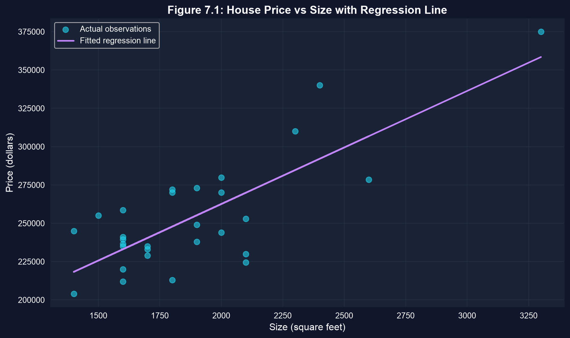
Inference quantifies the scatter: the larger the vertical gaps, the less precisely the slope is pinned down.

Direction: positive. Form: roughly linear. Scatter: residuals range from about −45,400 to +47,900 dollars. Note the one large house at 3,300 square feet: points far from the mean of x have high leverage and pull the line toward them. With only 29 houses, a single point like that matters for both the slope and its standard error.

7.2 · The t-statistic: signal over noise

Standard error of the slope · the \(T(n-2)\) distribution

Section 7.2: the standard error of the slope, what makes it large or small, and the t-statistic that standardizes the estimate.

The slope is a random variable

• Population: \(E[y \mid x] = \beta_1 + \beta_2 x\), with unknown \(\beta_2\)
• Sample: OLS gives \(b_2 = 73.77\), one draw from the sampling distribution of \(b_2\)
• Under assumptions 1–4: \(\;E[b_2] = \beta_2\) and \(\operatorname{Var}[b_2] = \dfrac{\sigma_u^2}{\sum_{i=1}^{n}(x_i - \bar x)^2}\)
• We never know \(\sigma_u^2\), so we replace it with \(s_e^2 = \dfrac{1}{n-2}\sum_{i=1}^{n}(y_i - \hat y_i)^2\)

\[\operatorname{se}(b_2) = \frac{s_e}{\sqrt{\sum_{i=1}^{n}(x_i - \bar x)^2}}\]

Standard deviation describes the spread of the data; standard error describes the spread of the estimate across samples.

The key distinction: SD is a property of the observations, SE is a property of the estimator. The variance formula is the classical one, valid under homoskedasticity and independence. We divide by n − 2 because two parameters (intercept and slope) were estimated from the same data, which uses up two degrees of freedom.

Three knobs set the standard error

\[\operatorname{se}(b_2) = \frac{s_e}{\sqrt{\sum (x_i - \bar x)^2}} \approx \frac{s_e}{\sqrt{n}\;s_x}\]

Knob	Turn it up	Effect on \(\operatorname{se}(b_2)\)
Residual spread \(s_e\)	worse fit, more noise	larger
Sample size \(n\)	more houses	smaller, at rate \(1/\sqrt n\): quadruple \(n\) to halve the SE
Spread of \(x\), \(s_x\)	wider range of sizes	smaller: extreme \(x\) values pin down the slope

A precise slope needs a tight fit, many observations and a wide spread in \(x\). All three are design choices, not luck.

The seesaw intuition from the chapter: the line pivots around the point of means. If the x values are spread widely, a small change in slope makes a big difference at the ends, so the data pin the slope down. If x values are bunched together, many slopes fit almost equally well. The approximation with √n·s_x is the chapter’s shortcut; the exact denominator is √(n−1)·s_x when s_x uses n − 1.

Code: build the standard error by hand

!pip install -q pyfixest                     # pyfixest is not preinstalled in Colab
import numpy as np                           # square roots and sums
import pandas as pd                          # tabular data
import pyfixest as pf                        # OLS with R-style formulas
url = "https://raw.githubusercontent.com/quarcs-lab/data-open/master/AED/AED_HOUSE.DTA"
data_house = pd.read_stata(url); model_basic = pf.feols("price ~ size", data=data_house)
n = len(data_house)                          # 29 houses
e = model_basic.resid()                      # residuals y - y_hat
s_e = np.sqrt((e**2).sum() / (n - 2))        # standard error of the regression
x = data_house["size"]                       # the regressor
sxx = ((x - x.mean())**2).sum()              # total variation in x
se_formula = s_e / np.sqrt(sxx)              # classical se(b2), exact
se_shortcut = s_e / (np.sqrt(n) * x.std())   # chapter's shortcut with sqrt(n)
print(s_e, np.sqrt(sxx), se_formula, se_shortcut, model_basic.se()["size"])

↗ Try it in Colab

Self-contained. resid() returns the OLS residuals. The exact formula reproduces pyfixest’s standard error to every decimal; the shortcut is slightly smaller because it uses √n where the exact expression implies √(n − 1).

Output: the formula reproduces the table exactly

Ingredient	Value
\(s_e\), standard error of the regression	23,550.66
\(\sqrt{\sum (x_i - \bar x)^2}\)	2,107.46
\(s_x\), SD of size	398.27
\(\operatorname{se}(b_2) = s_e / \sqrt{\sum (x_i - \bar x)^2}\)	11.175
Shortcut \(s_e / (\sqrt{n}\, s_x)\)	10.98
pyfixest se()["size"]	11.175

\(23{,}550.66 / 2{,}107.46 = 11.175\): nothing in the regression table is a black box.

The typical house is about 23,551 dollars away from the fitted line. Dividing by the square root of the total variation in size gives the standard error of 11.175 dollars per square foot. The shortcut gives 10.98 because √29 × 398.27 is a bit larger than √28 × 398.27 = √Σ(x − x̄)². The chapter’s claim that with R² = 0.10 instead of 0.62 the SE would be about 1.5 times larger checks out: √(0.90/0.383) = 1.53, holding the variance of price fixed.

The \(t\)-statistic standardizes the estimate

\[t = \frac{b_2 - \beta_2^{*}}{\operatorname{se}(b_2)} \;\sim\; T(n-2) \quad\text{under } H_0: \beta_2 = \beta_2^{*}\]

• If we knew \(\sigma_u\), the ratio would be standard normal, \(N(0,1)\)
• Estimating \(\sigma_u\) by \(s_e\) adds extra uncertainty, so the ratio follows Student’s \(t\) with \(n - 2\) degrees of freedom
• For \(H_0: \beta_2 = 0\): \(\;t = \dfrac{73.77}{11.17} = 6.60\)

\(t = 6.60\) means the slope sits 6.6 of its own standard errors above zero.

Degrees of freedom: 29 observations minus 2 estimated parameters = 27. This is the bivariate counterpart of the univariate t-statistic from Chapter 4, (x̄ − μ)/se(x̄) ~ T(n − 1). The only difference is that one more parameter is estimated, so one more degree of freedom is used up.

Code: extract the ingredients of \(t\)

# continues from the previous block (model_basic already fitted)
coef_size = model_basic.coef()["size"]       # b2
se_size = model_basic.se()["size"]           # se(b2)
t_stat_size = model_basic.tstat()["size"]    # t for H0: beta2 = 0
p_value_size = model_basic.pvalue()["size"]  # two-sided p-value
print(f"t = b2 / se(b2) = {coef_size:.4f} / {se_size:.4f} = {t_stat_size:.4f}")
print(f"p-value: {p_value_size:.6f}")        # prints 0.000000 at 6 decimals

↗ Try it in Colab

Output: \(t = 73.7710 / 11.1749 = 6.6015\); \(p = 4.4 \times 10^{-7}\), which prints as 0.000000.

coef(), se(), tstat() and pvalue() each return a pandas Series indexed by variable name. The p-value is so small that six decimal places show only zeros; it is not literally zero, so write p < 0.001 rather than p = 0.000.

Scorecard after 7.2

Question	Answer for the house slope
Is it precise?	\(\operatorname{se}(b_2) = 11.17\): about 15% of the estimate
Is it real?	\(t = 6.60\), far beyond any conventional cutoff
Does it matter?	to be judged in 7.4
Is the SE honest?	classical SE so far; checked in 7.7

Precision is relative: an SE of 11 is small next to a slope of 74, and it would be huge next to a slope of 5.

The scorecard is the deck’s recurring thread. It fills in as we go: by 7.7 every row will be answered for the house slope, and the two case studies get their own scorecards. The ratio of the SE to the estimate, 11.17/73.77 = 0.15, is the inverse of the t-statistic.

7.3 · Confidence intervals: the slopes the data cannot rule out

Estimate ± critical value × standard error

Section 7.3: building, computing and correctly interpreting a confidence interval for the slope, and why the t-distribution rather than the normal.

A confidence interval is estimate ± margin of error

\[b_2 \;\pm\; t_{n-2,\,\alpha/2}\times\operatorname{se}(b_2)\]

\[73.77 \;\pm\; 2.052 \times 11.17 \;=\; 73.77 \pm 22.93 \;=\; [50.84,\ 96.70]\]

• \(t_{27,\,0.025} = 2.052\): the value that leaves 2.5% in each tail of \(T(27)\)
• Margin of error 22.93: the half-width of the interval
• Quick approximation: \(b_2 \pm 2\times\operatorname{se}(b_2)\)

The interval spans $46 per square foot: size clearly matters, but its price is pinned down only to “somewhere between $51 and $97”.

The general recipe from Chapter 4 carries over: estimate ± critical value × standard error. With 27 degrees of freedom the 95% critical value is 2.052 rather than 1.96. The width, 2 × 22.93 = 45.86 dollars, is the honest summary of how much 29 houses can tell us.

Code: the interval from pyfixest and by hand

!pip install -q pyfixest                     # pyfixest is not preinstalled in Colab
import pandas as pd, pyfixest as pf          # data and OLS
from scipy import stats                      # Student's t quantiles
url = "https://raw.githubusercontent.com/quarcs-lab/data-open/master/AED/AED_HOUSE.DTA"
data_house = pd.read_stata(url); model_basic = pf.feols("price ~ size", data=data_house)
print(model_basic.confint())                 # 95% CIs for intercept and slope
df = len(data_house) - 2                     # 27 degrees of freedom
t_crit = stats.t.ppf(0.975, df)              # 2.5% in the upper tail
b2, se2 = model_basic.coef()["size"], model_basic.se()["size"]
ci_lower, ci_upper = b2 - t_crit * se2, b2 + t_crit * se2   # estimate ± margin
print(t_crit, t_crit * se2, ci_lower, ci_upper)
z_lo, z_hi = b2 - 1.96 * se2, b2 + 1.96 * se2  # normal-based interval, for comparison

↗ Try it in Colab

Self-contained. stats.t.ppf(0.975, 27) is the 97.5th percentile of T(27). The last line is not in the chapter: it computes the interval we would get by wrongly using the normal critical value, to show the difference on the next slide.

Output: the manual interval matches confint() exactly

Quantity	\(t(27)\)-based	Normal-based (for comparison)
Critical value	2.052	1.960
Margin of error	22.93	21.90
95% CI for \(\beta_2\)	[50.84, 96.70]	[51.87, 95.67]

confint() returns [50.84, 96.70] for size and [70,924.76, 159,109.81] for the intercept · normal column computed for these slides

With 27 degrees of freedom, the correct interval is 4.7% wider than the normal one: a small but real penalty for estimating \(\sigma_u\).

2.052/1.960 = 1.047, so the t-based margin is 4.7% wider (the chapter rounds this to 5%). Software always uses the t-distribution; the normal column is only there to show what is at stake. In large samples the two columns converge.

Small samples need heavier tails

Standard normal vs \(T(27)\) and \(T(3)\), with their 5% two-sided critical values.

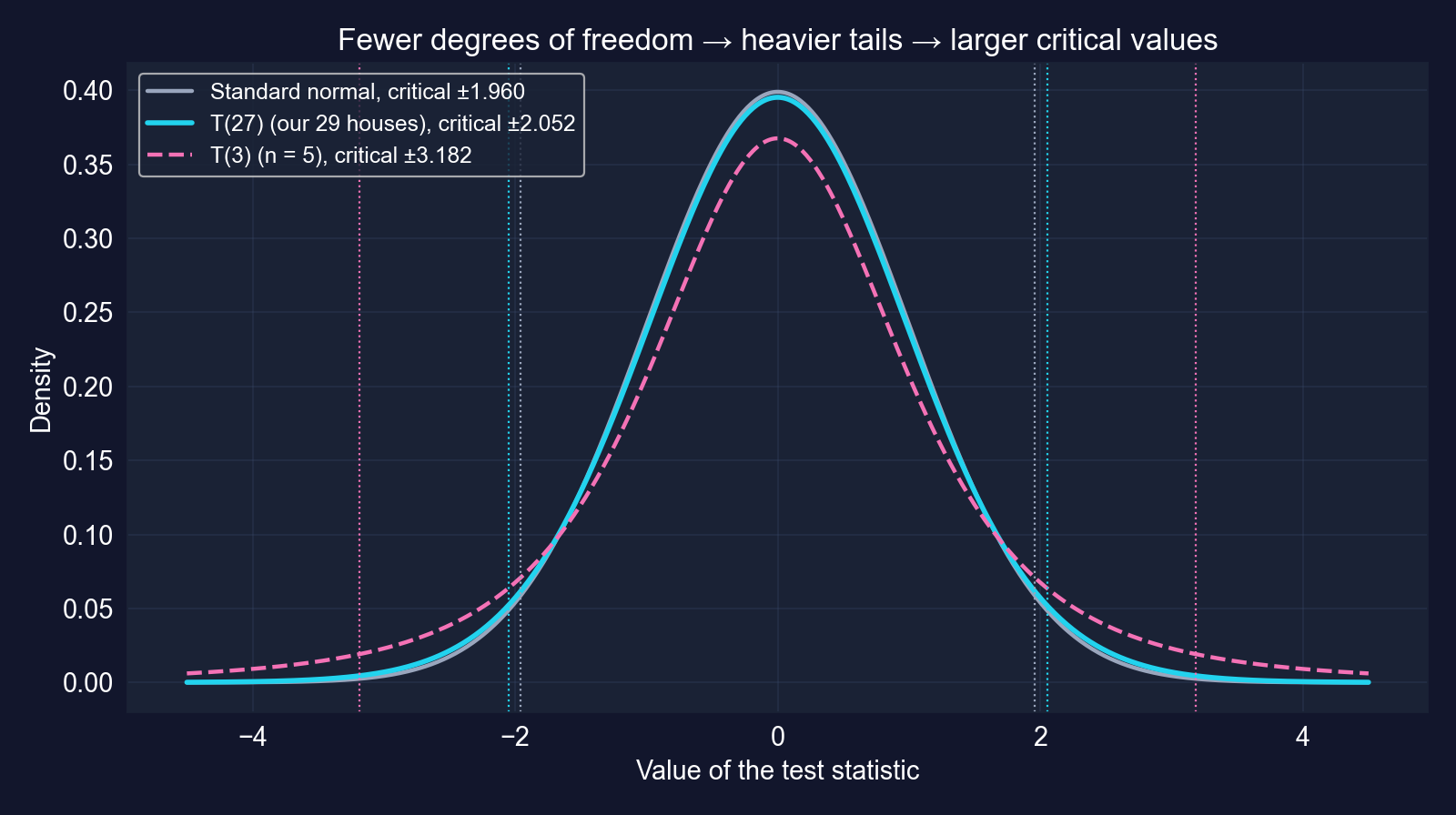
\(n\)	df	\(t_{\text{df},\,0.025}\)	vs 1.960
5	3	3.182	+62%
10	8	2.306	+18%
29	27	2.052	+5%
30	28	2.048	+5%
100	98	1.984	+1%
\(\infty\)	—	1.960	0%

Fewer degrees of freedom mean heavier tails, larger critical values and wider intervals. Above about 100 observations the difference is negligible.

The t-distribution is symmetric and bell-shaped like the normal, with variance df/(df − 2) > 1, so more probability sits in the tails. As df grows it converges to the normal. Rule from the chapter: always use t, because software does and it is correct for any n; it matters most below about 30 observations. The chapter’s table lists n = 30 with 2.048 (+4%); computed exactly, 2.048/1.960 = 1.045, so the slide rounds it to +5%.

The confidence level trades certainty for width

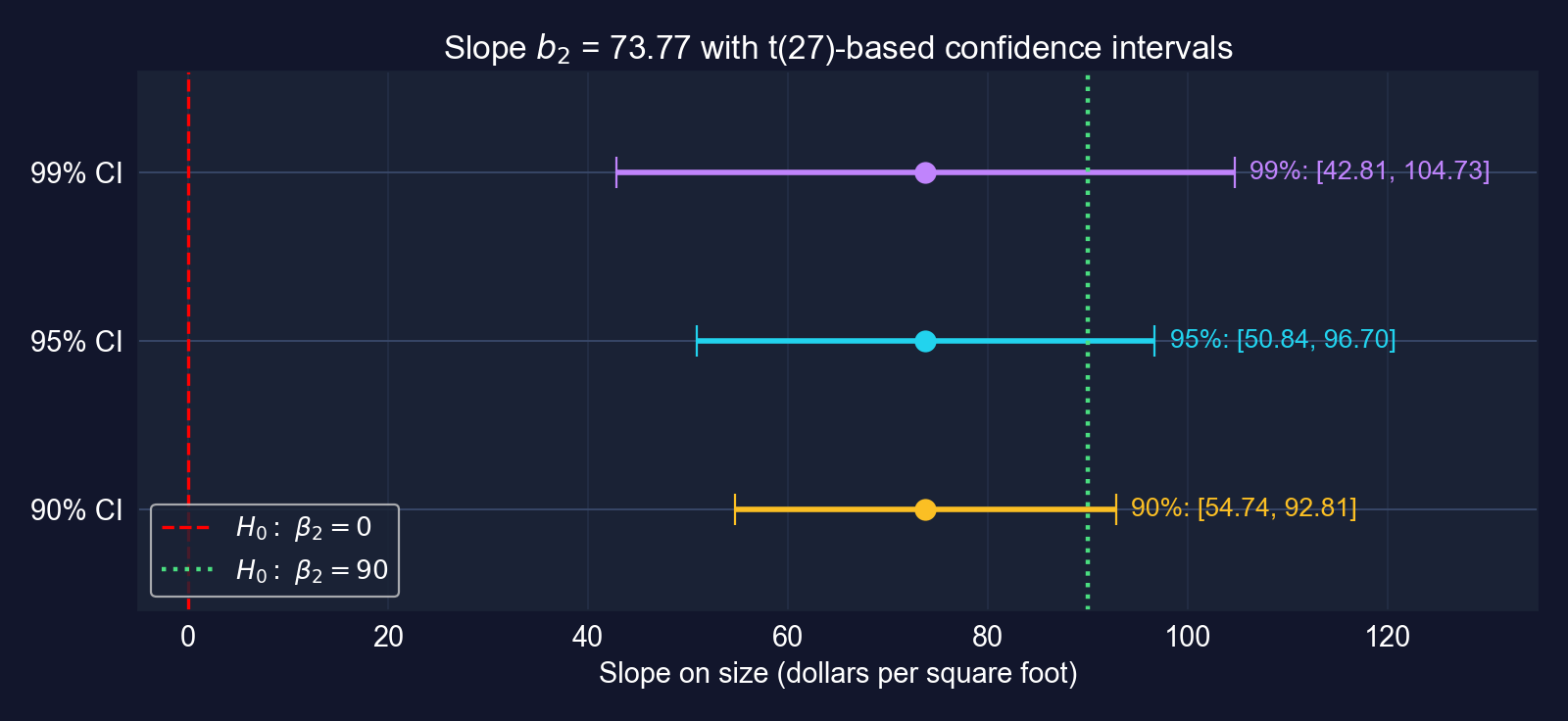
The same slope with 90%, 95% and 99% intervals. Zero is outside all three; 90 is inside all three.

90%: [54.74, 92.81] · 95%: [50.84, 96.70] · 99%: [42.81, 104.73]. Asking for more confidence buys a wider, less informative range.

Critical values: 1.703 for 90%, 2.052 for 95%, 2.771 for 99%, all with 27 df. The 90% and 99% intervals are computed for these slides from the same estimate and SE. Notice that $90 per square foot is inside every interval, which previews the test in Section 7.5. Notice also that the 90% interval’s upper end, 92.81, is close to 90, which previews the one-sided test in 7.6.

What “95% confidence” does and does not mean

• Wrong: “there is a 95% probability that \(\beta_2\) lies between 50.84 and 96.70”
• Right: if we drew many samples and built an interval from each, about 95% of those intervals would contain \(\beta_2\)
• \(\beta_2\) is a fixed number; the interval is what varies from sample to sample
• Our interval [50.84, 96.70] either contains \(\beta_2\) or it does not; 95% describes the procedure’s long-run success rate

Width depends on three things: the confidence level, the sample size (through both the SE and the critical value) and the residual noise.

This is the chapter’s Key Concept 7.2. The frequentist interpretation is subtle, and the wrong version is very common, even in published work. A useful way to say it in words: “the procedure that produced this interval captures the true slope 95% of the time”. The next slide makes the idea visible with a simulation.

100 samples, 100 intervals: about 95 cover the truth

Simulated illustration, not chapter data: 100 samples of 29 houses drawn from a population whose true slope is 73.77, each with its 95% interval.

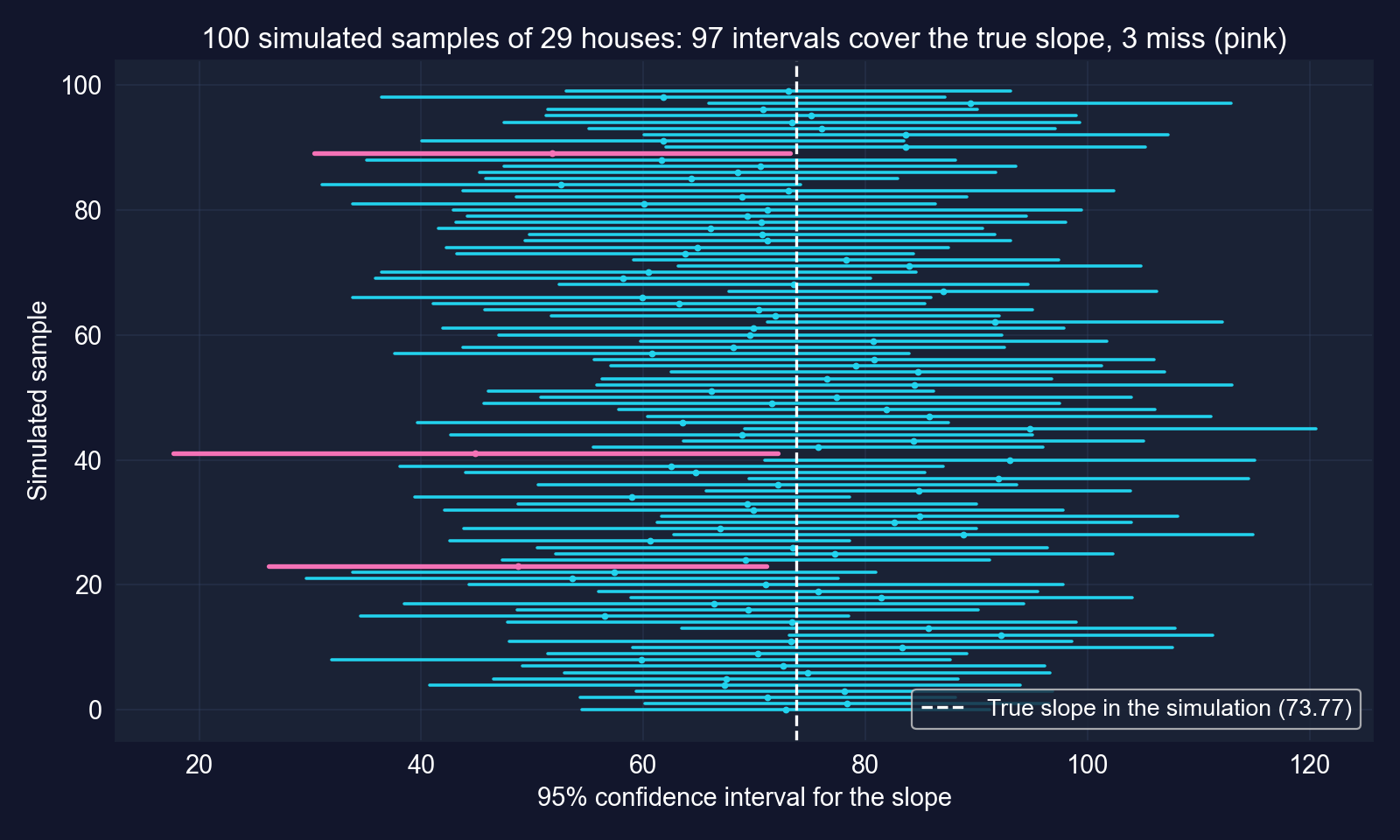
In this simulation, 97 of 100 intervals contain the true slope and 3 miss it. The 95% is a property of the procedure.

Built for these slides. The simulation keeps the 29 house sizes, sets the true intercept and slope equal to the chapter’s estimates, draws normal errors with SD equal to s_e = 23,551, re-estimates the regression 100 times and builds a t-based 95% interval each time. 97 cover the truth; with a different seed you would get a number near 95. In real life we see only one of these lines and never know whether it is one of the misses.

With five observations, the interval balloons

# continues from the previous block (pd, pf, stats already imported)
df_artificial = pd.DataFrame({"x": [1, 2, 3, 4, 5],    # the chapter's artificial data
                              "y": [1, 2, 2, 2, 3]})
model_artificial = pf.feols("y ~ x", data=df_artificial)   # OLS on 5 points
coef_x, se_x = model_artificial.coef()["x"], model_artificial.se()["x"]
t_crit_art = stats.t.ppf(0.975, 5 - 2)                 # only 3 degrees of freedom
print(coef_x, se_x, t_crit_art)                        # slope, SE, critical value
print(coef_x - t_crit_art * se_x, coef_x + t_crit_art * se_x)  # 95% CI

↗ Try it in Colab

\(b_2\)	SE	\(t\)	\(t_{3,\,0.025}\)	95% CI
0.400	0.115	3.46	3.182	[0.03, 0.77]

Even with \(t = 3.46\), the interval runs from almost zero to almost double the estimate: with 3 degrees of freedom the critical value is 3.182, not 1.96.

The chapter’s artificial example. The slope 0.40 is significant at 5% (p = 0.041) but only just: the interval’s lower end is 0.03. Compare with the house data, where the critical value is 2.052. Small samples are doubly penalized: a larger standard error and a larger critical value.

7.4 · Is the slope different from zero?

Tests of statistical significance · \(p\)-values · economic significance

Section 7.4: the test of statistical significance, the p-value and the critical-value rules, and the crucial difference between statistical and economic significance.

The test of statistical significance

\[H_0: \beta_2 = 0 \qquad\text{vs.}\qquad H_a: \beta_2 \neq 0, \qquad t = \frac{b_2}{\operatorname{se}(b_2)} \sim T(n-2) \text{ under } H_0\]

• \(p\)-value rule: reject \(H_0\) at level \(\alpha\) if \(p = \Pr\big[\,|T_{n-2}| > |t|\,\big] < \alpha\)
• Critical-value rule: reject \(H_0\) if \(|t| > t_{n-2,\,\alpha/2}\)
• The two rules always agree; \(\alpha\) is the probability of a Type I error (rejecting a true \(H_0\))
• Never “accept” \(H_0\): we either reject it or fail to reject it

A regressor “matters” statistically when its coefficient is too far from zero to blame on sampling noise.

The five-step workflow from Key Concept 7.3: state H0 and Ha, choose α (usually 0.05), compute the test statistic, find the p-value, decide, and then translate the decision into plain language. The null is the claim we try to overturn; the burden of proof is on the data.

Code: run the test both ways

!pip install -q pyfixest                     # pyfixest is not preinstalled in Colab
import pandas as pd, pyfixest as pf; from scipy import stats
url = "https://raw.githubusercontent.com/quarcs-lab/data-open/master/AED/AED_HOUSE.DTA"
data_house = pd.read_stata(url); model_basic = pf.feols("price ~ size", data=data_house)
t_stat_size = model_basic.tstat()["size"]    # b2 / se(b2)
p_value_size = model_basic.pvalue()["size"]  # Pr[|T27| > |t|]
t_crit = stats.t.ppf(0.975, len(data_house) - 2)       # 5% two-sided cutoff
print(t_stat_size, p_value_size, t_crit)
print("Reject H0" if p_value_size < 0.05 else "Fail to reject H0")

↗ Try it in Colab

Self-contained. The p-value approach compares p with α; the critical-value approach compares |t| with 2.052. Both lead to the same decision because they are the same comparison expressed on two scales.

Output: size is significant at any conventional level

\(H_0\)	\(t\)	\(p\) (two-sided)	Critical value, 5%	Decision
\(\beta_2 = 0\)	6.60	\(4.4\times 10^{-7}\)	±2.052	reject

• \(|t| = 6.60 > 2.052\), and \(p < 0.001\): reject at 5%, 1% and far beyond
• Reading the \(p\)-value: if \(\beta_2\) were really 0, a \(|t|\) this large would occur in fewer than 1 in a million samples
• It is not the probability that \(H_0\) is true, and it does not measure how large the effect is

Conclusion in words: in Davis in 1999, larger houses sold for more, and the association is far too strong to be a fluke of this sample.

p = 4.4 × 10⁻⁷, so the probability is about 0.44 in a million under the null. Software that prints 0.000 is rounding. The chapter’s p-value table labels 0.01 < p ≤ 0.05 “significant” and 0.05 < p ≤ 0.10 “marginally significant”; these are conventions, not laws, and p = 0.049 and p = 0.051 carry essentially the same evidence (Key Concept 7.8).

Statistically significant does not mean important

Statistical significance

• Is the effect distinguishable from zero?
• Driven by \(t = b_2/\operatorname{se}(b_2)\), so by \(n\), noise and spread in \(x\)
• With a huge \(n\), even a trivial effect is “significant”

Economic significance

• Is the effect large enough to matter?
• Driven by the magnitude of \(b_2\), in context
• Needs domain knowledge, not a table of critical values

Report the magnitude and its confidence interval, not just the stars. The interval answers both questions at once.

Key Concept 7.4. Two failure modes: a precisely estimated but tiny effect (statistically significant, economically trivial), and a large but imprecise effect (economically important, statistically insignificant). The chapter’s job-training example: a wage gain of 50 cents an hour (p = 0.001) is about 1,000 dollars a year at 2,000 hours, which is worth it if the programme costs 500 dollars and not if it costs 10,000.

Is $73.77 per square foot economically large?

Comparison	Implied price difference	Using the 95% CI
10 extra square feet	$738	—
100 extra square feet	$7,377	[$5,084, $9,670]
One SD of size (398 sq ft)	$29,381	11.6% of the mean price

100 sq ft rows: chapter · CI and one-SD rows computed for these slides from \(b_2\) and its interval

Even the lower end of the interval, about $5,100 per 100 square feet, is a meaningful sum on a $254,000 house: the effect is both statistically and economically significant.

The chapter computes 7,377 dollars for 100 square feet and about 738 dollars for 10 square feet. Multiplying the CI by 100 gives the range 5,084 to 9,670. A one-SD difference in size (398 square feet) goes with 29,381 dollars, about 11.6% of the mean price of 253,910 dollars. Economic significance is a judgment; these comparisons give the judgment something concrete to work with. Remember this is an association across houses, not the value of adding a room.

7.5 · Is the slope $90 per square foot?

Two-sided tests of a specific value · the CI–test duality

Section 7.5: testing whether the slope equals a specific non-zero value, and why that is the same as asking whether the value lies inside the confidence interval.

Testing a specific value: same recipe, new null

\[H_0: \beta_2 = 90 \qquad\text{vs.}\qquad H_a: \beta_2 \neq 90\]

\[t = \frac{b_2 - 90}{\operatorname{se}(b_2)} = \frac{73.77 - 90}{11.17} = -1.452\]

• Two-sided \(p = \Pr\big[\,|T_{27}| > 1.452\,\big]\)
• Reject at 5% only if \(|t| > 2.052\)
• Where could 90 come from? A realtor’s rule of thumb, a building-cost benchmark, a previous study

Only the numerator changes: the test asks how many standard errors the estimate is from the claimed value.

The test of significance is the special case β2* = 0. Any economically interesting benchmark can be tested the same way. The sign of t tells you which side of the claim the estimate falls on: here the estimate is 16.23 dollars below 90.

Code: test \(H_0: \beta_2 = 90\)

!pip install -q pyfixest                     # pyfixest is not preinstalled in Colab
import pandas as pd, pyfixest as pf; from scipy import stats
url = "https://raw.githubusercontent.com/quarcs-lab/data-open/master/AED/AED_HOUSE.DTA"
data_house = pd.read_stata(url); model_basic = pf.feols("price ~ size", data=data_house)
null_value, df = 90, len(data_house) - 2     # claimed slope; 27 degrees of freedom
coef_size, se_size = model_basic.coef()["size"], model_basic.se()["size"]
t_stat_90 = (coef_size - null_value) / se_size              # distance from 90 in SEs
p_value_90 = 2 * (1 - stats.t.cdf(abs(t_stat_90), df))      # two-sided p-value
print(t_stat_90, p_value_90, stats.t.ppf(0.975, df))        # t, p, critical value
print(model_basic.confint().loc["size"])                    # is 90 inside the CI?

↗ Try it in Colab

Self-contained. stats.t.cdf gives the probability below |t|; one minus that, doubled, is the two-sided tail area. The last line prints the interval so the duality can be checked by eye.

Output: $90 per square foot is consistent with the data

	Value
\(t\)	−1.452
\(p\) (two-sided)	0.158
Critical value	±2.052
95% CI	[50.84, 96.70]
Decision at 5%	do not reject

Left: \(t = 6.60\) lands deep in the rejection region. Right: \(t = -1.45\) does not; the hatched area is the \(p\)-value.

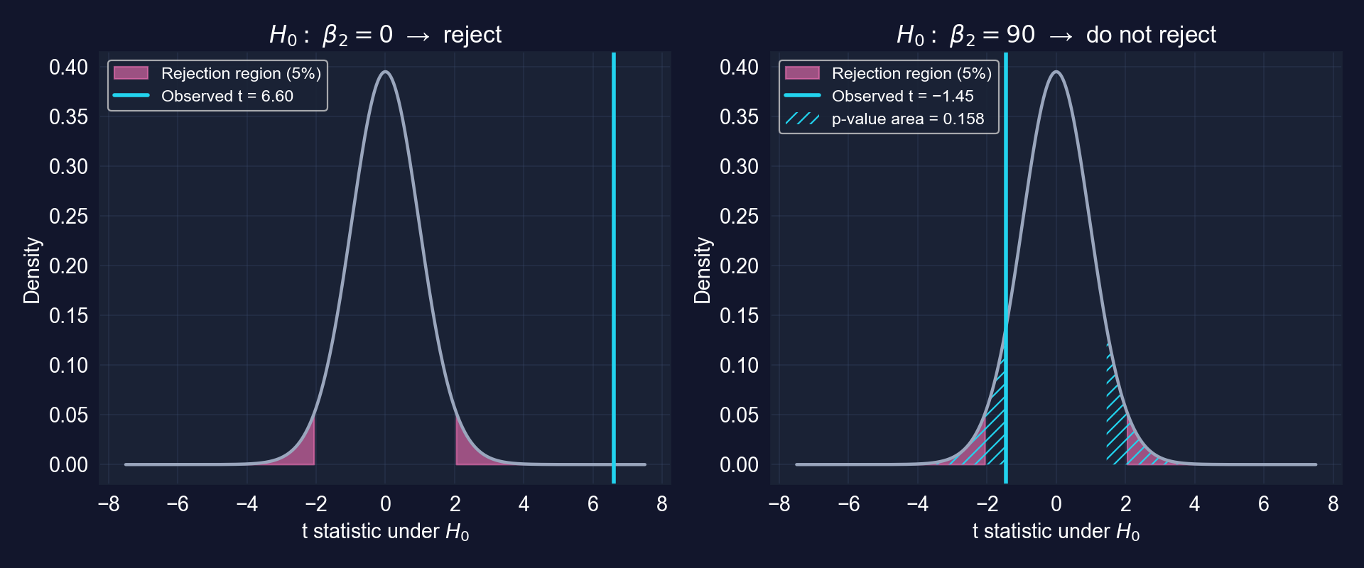
\(p = 0.158 > 0.05\) and 90 lies inside [50.84, 96.70]: two ways of saying the same thing.

If the true slope were 90, an estimate at least 16.23 dollars away from 90 (in either direction) would occur in about 16% of samples, which is not unusual. The figure puts the two tests side by side on the same T(27) density: the test of zero rejects overwhelmingly, the test of 90 does not.

A confidence interval is a family of tests

• Reject \(H_0: \beta_2 = \beta_2^{*}\) at 5% exactly when \(\beta_2^{*}\) is outside the 95% CI
• 0 is outside [50.84, 96.70] → reject; 90 is inside → do not reject
• But 60, 75 and 95 are inside too: the data are consistent with all of them
• “Do not reject \(\beta_2 = 90\)” does not mean “\(\beta_2 = 90\)”

Failing to reject is a statement about the data’s power, not proof of the null. Report the interval and every plausible value is visible at once.

Key takeaway 4 of the chapter. The duality makes confidence intervals more informative than a single test: one interval answers every two-sided test at once. A common mistake is to read “fail to reject” as “accept”: with 29 houses the data cannot distinguish 90 from 60. Key Concept 7.9: never conclude “proved β2 = 90”.

7.6 · Is the slope less than $90?

One-sided directional tests

Section 7.6: directional hypotheses, where the rejection region sits in only one tail, and the conditions under which the two-sided p-value can be halved.

One-sided tests put the claim in the alternative

Test	\(H_0\)	\(H_a\) (the claim)	Reject when	\(p\)-value
Upper tail	\(\beta_2 \le \beta_2^{*}\)	\(\beta_2 > \beta_2^{*}\)	\(t > t_{n-2,\,\alpha}\)	\(\Pr[T_{n-2} > t]\)
Lower tail	\(\beta_2 \ge \beta_2^{*}\)	\(\beta_2 < \beta_2^{*}\)	\(t < -t_{n-2,\,\alpha}\)	\(\Pr[T_{n-2} < t]\)

• The claim you want to demonstrate goes in \(H_a\), so the data must prove it
• The whole 5% sits in one tail: \(t_{27,\,0.05} = 1.703\) instead of 2.052
• Choose the direction before seeing the data, from theory

A one-sided test has more power in the predicted direction, and none at all in the other.

Key Concept 7.5. One-sided tests are appropriate when theory predicts the direction and you only care about deviations in that direction. Journals usually expect two-sided tests, partly because choosing the direction after looking at the estimate is a form of fishing.

Code: both one-sided tests of 90

!pip install -q pyfixest                     # pyfixest is not preinstalled in Colab
import pandas as pd, pyfixest as pf; from scipy import stats
url = "https://raw.githubusercontent.com/quarcs-lab/data-open/master/AED/AED_HOUSE.DTA"
data_house = pd.read_stata(url); model_basic = pf.feols("price ~ size", data=data_house)
df = len(data_house) - 2                     # 27 degrees of freedom
t_stat_90 = (model_basic.coef()["size"] - 90) / model_basic.se()["size"]
p_value_upper = 1 - stats.t.cdf(t_stat_90, df)   # Ha: beta2 > 90 (right tail)
p_value_lower = stats.t.cdf(t_stat_90, df)       # Ha: beta2 < 90 (left tail)
t_crit_one = stats.t.ppf(0.95, df)               # one-sided 5% critical value
print(t_stat_90, p_value_upper, p_value_lower, t_crit_one)

↗ Try it in Colab

Self-contained. Same t-statistic as the two-sided test; only the tail area changes. The chapter’s cell runs both directions to show the asymmetry.

Output: the direction of the claim decides everything

	Lower tail	Upper tail
\(H_a\)	\(\beta_2 < 90\)	\(\beta_2 > 90\)
\(t\)	−1.452	−1.452
\(p\)	0.079	0.921
Cutoff, 5%	−1.703	+1.703
Decision	do not reject	do not reject

Left: the claim \(\beta_2 < 90\); the estimate leans its way but not far enough. Right: the claim \(\beta_2 > 90\); the estimate points the other way.

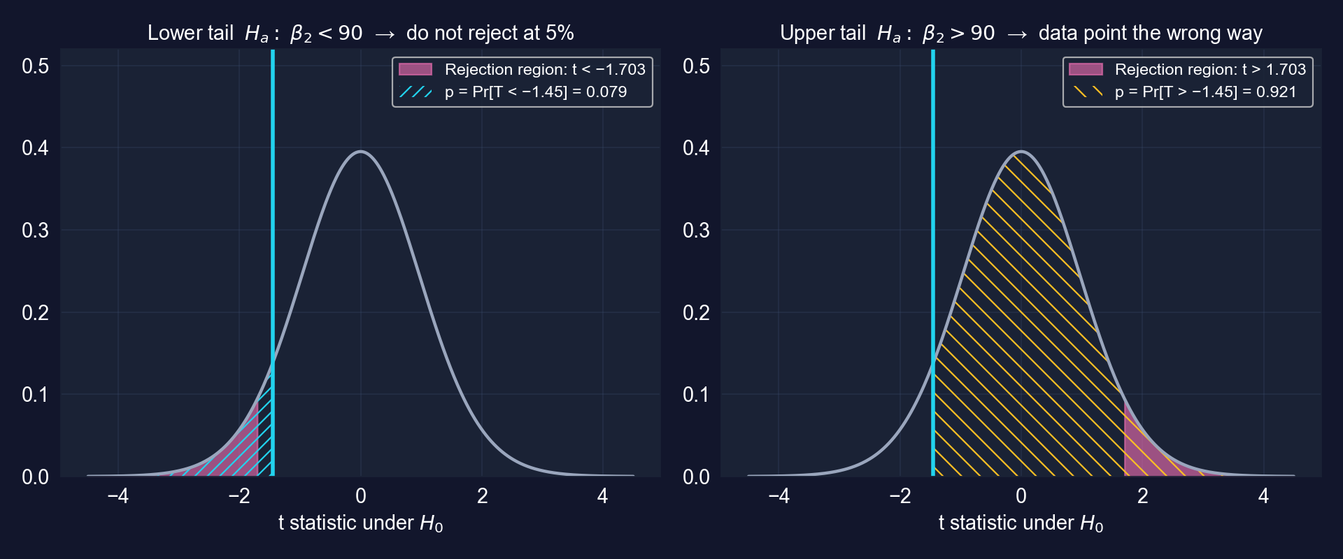
The evidence that the slope is below $90 is suggestive (\(p = 0.079\)): not enough at 5%, enough at 10%. The evidence that it is above $90 is nil (\(p = 0.921\)).

The lower-tail p-value 0.079 is half the two-sided 0.158, because the estimate (73.77) lies on the side of the claim (below 90). The upper-tail p-value is 1 − 0.079 = 0.921, above 0.5, because the estimate lies on the wrong side of the claim. Halving the two-sided p-value is valid only in the first situation.

Halve the \(p\)-value only when the estimate points your way

• Software reports two-sided \(p\)-values for \(H_0: \beta_2 = 0\)
• One-sided test of significance: if \(b_2\) has the predicted sign, one-sided \(p\) = two-sided \(p\) / 2
• If \(b_2\) has the wrong sign, one-sided \(p > 0.5\): rejection is impossible
• House example: \(H_a: \beta_2 > 0\) gives \(p = 2.2\times 10^{-7}\), half of \(4.4\times 10^{-7}\)

An earlier version of this deck halved the \(p\)-value for \(H_a: \beta_2 > 90\). That is wrong: with \(b_2 = 73.77 < 90\) the correct one-sided \(p\) is 0.921.

The halving rule has a condition attached, and dropping the condition is a common slip. The chapter states it correctly (“if sign is correct”) and its code computes both tails. Practical advice: decide the direction from theory before estimation, and when in doubt report the two-sided test.

7.7 · Are the standard errors honest?

Heteroskedasticity · HC1 robust standard errors · residual diagnostics

Section 7.7: what happens to inference when the error variance is not constant, and how heteroskedasticity-robust standard errors fix it.

Heteroskedasticity breaks the classical standard error

Assumption 3 says \(\operatorname{Var}[u_i \mid x_i] = \sigma_u^2\) for every observation. Heteroskedasticity: \(\operatorname{Var}[u_i \mid x_i] = \sigma_i^2\) varies with \(i\).

What	Under heteroskedasticity
Coefficient \(b_2\)	still unbiased and consistent
Classical \(\operatorname{se}(b_2)\)	wrong, too small or too large
\(t\), \(p\), confidence intervals	invalid (wrong size, wrong coverage)

The fix leaves the estimate alone and repairs the uncertainty: a heteroskedasticity-robust standard error.

Heteroskedasticity is common in cross-sections: spending varies more among rich households, sales vary more among large firms, house prices vary more among large houses. The direction of the bias in the classical SE depends on the pattern, so we cannot predict it without knowing the form. Robust SEs are valid whether or not heteroskedasticity is present, but this is a large-sample result: with only n = 29 houses they are approximately valid.

Classical vs robust: one formula, one change

\[\operatorname{se}(b_2) = \frac{s_e}{\sqrt{\sum (x_i - \bar x)^2}} \qquad\qquad \operatorname{se}_{\text{HC0}}(b_2) = \frac{\sqrt{\sum e_i^2\,(x_i - \bar x)^2}}{\sum (x_i - \bar x)^2}\]

• Classical: one pooled residual variance \(s_e^2\) for every observation
• Robust (White / Huber–White): each squared residual \(e_i^2\) is weighted by that observation’s leverage \((x_i - \bar x)^2\)
• HC1 = HC0 × \(\sqrt{n/(n-k)}\), a degrees-of-freedom correction; with \(n = 29\), \(k = 2\) the factor is 1.036
• Variants: HC2 (leverage-weighted), HC3 (more conservative); HAC for time series, cluster-robust for grouped data

The chapter prints the HC0 formula (10.93 for the house slope), but its code and tables use HC1 (vcov="HC1", 11.33), which matches Stata’s robust.

Large residuals at extreme x values are exactly what the classical formula misses. HC1 multiplies the HC0 variance by n/(n − k); for the house data, HC0 = 10.932 and HC1 = 10.932 × √(29/27) = 11.330. This deck labels the formula as HC0 and reports HC1 numbers, so the two are not confused.

Code: re-estimate with HC1 robust standard errors

!pip install -q pyfixest                     # pyfixest is not preinstalled in Colab
import pandas as pd, pyfixest as pf          # data and OLS
url = "https://raw.githubusercontent.com/quarcs-lab/data-open/master/AED/AED_HOUSE.DTA"
data_house = pd.read_stata(url)
model_basic = pf.feols("price ~ size", data=data_house)              # classical SEs
robust_results = pf.feols("price ~ size", data=data_house, vcov="HC1")  # robust SEs
comparison_df = pd.DataFrame({
    "Coefficient": model_basic.coef(),            # identical in both fits
    "Std. Error": model_basic.se(),               # classical
    "Robust SE": robust_results.se(),             # HC1
    "t-stat (standard)": model_basic.tstat(),
    "t-stat (robust)": robust_results.tstat(),
})
print(comparison_df); robust_results.summary()   # full table reports "Inference: HC1"

↗ Try it in Colab

Self-contained. pyfixest’s default is classical (iid) standard errors; vcov=“HC1” requests heteroskedasticity-robust ones. The coefficients are computed exactly as before; only the variance estimate changes.

Output: the slope’s SE barely moves

Variable	Coef.	Classical SE	Robust SE	Change	Robust \(t\)	Robust 95% CI
Intercept	115,017.3	21,489.4	20,298.7	−5.5%	5.67	[73,368, 156,667]
size	73.771	11.175	11.330	+1.4%	6.51	[50.52, 97.02]

N = 29 · HC1 SEs · robust \(p < 0.001\) for both coefficients · \(R^2 = 0.617\) (unchanged)

Same coefficient, two standard errors: the 95% intervals almost coincide, and both contain 90.

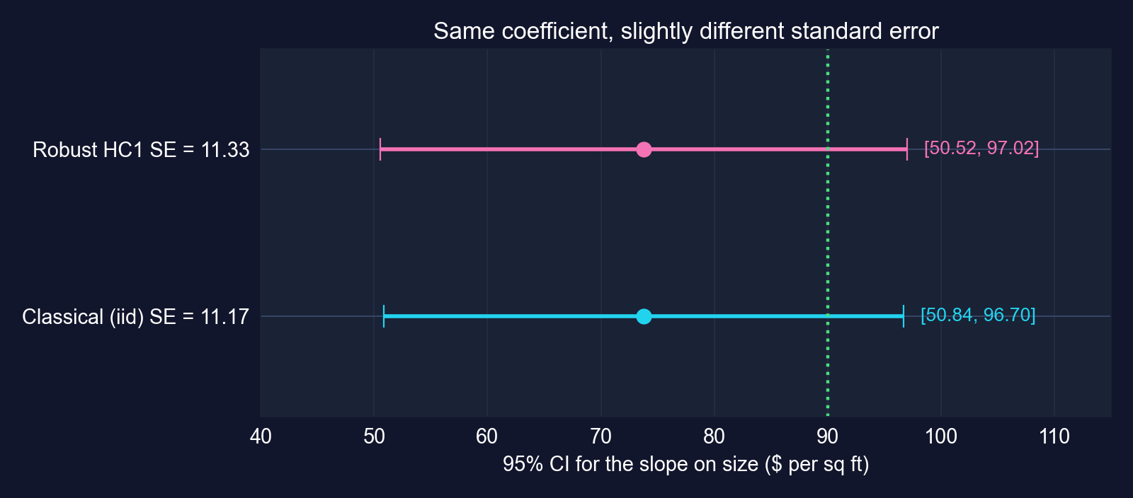
Robust inference reaches the same verdicts: size is significant (\(t = 6.51\)), and $90 is still not rejected (robust \(t = -1.43\), \(p = 0.163\)).

The robust SE is 1.4% larger for the slope and 5.5% smaller for the intercept: robust SEs are usually but not always larger. The robust test of 90 (computed for these slides) gives t = −1.432 and p = 0.163, against −1.452 and 0.158 with classical SEs. With such a small change, heteroskedasticity is not distorting inference here. Rule of thumb from the chapter: differences under 10% suggest little heteroskedasticity; differences over 20% demand robust SEs.

Residual check: no strong funnel, but only 29 points

Residuals against fitted values (chapter Figure 7.3).

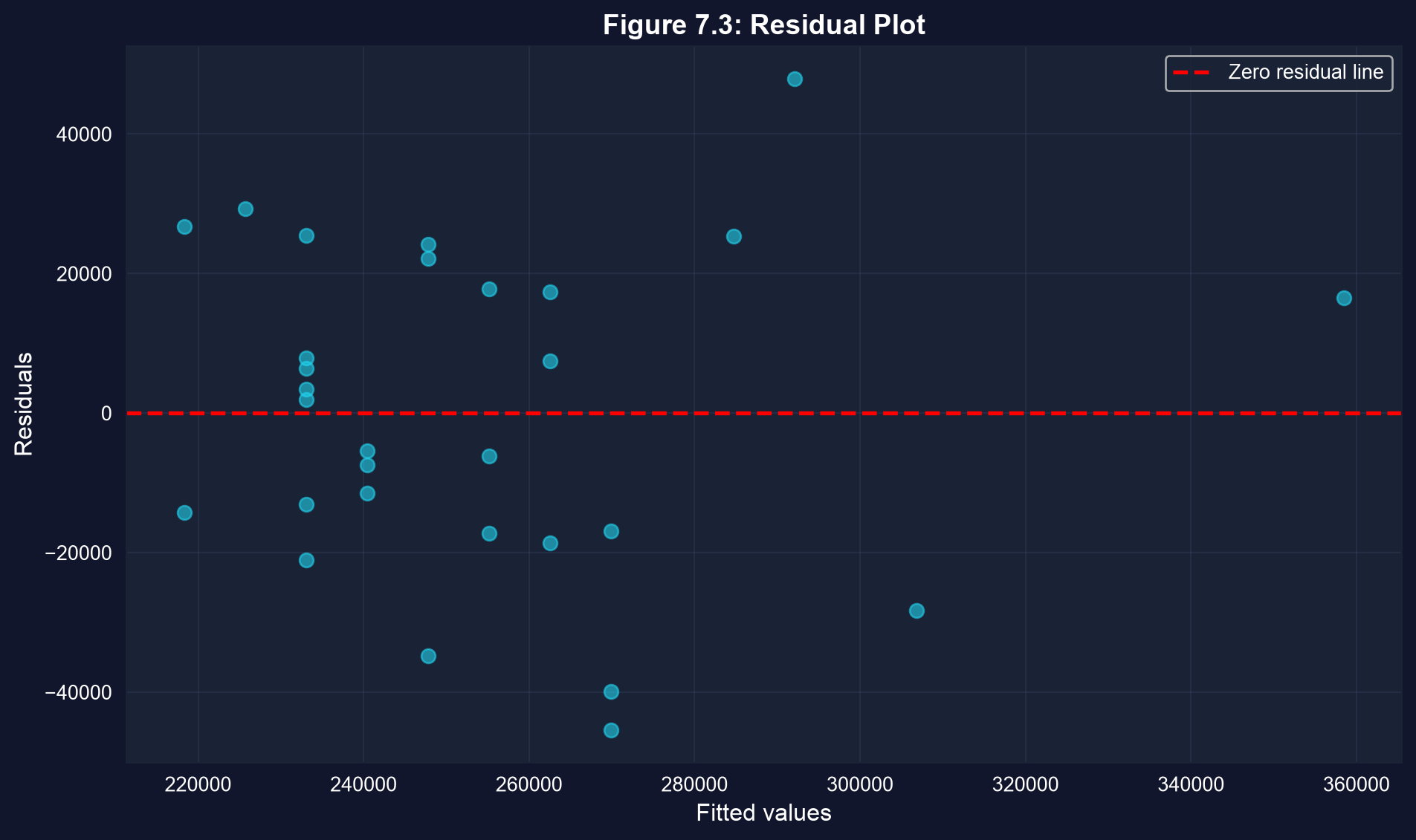
Fitted value	Houses	Residual SD
at or below median	16	$19,258
above median	13	$27,670

Split computed for these slides; ties at the median make the halves unequal.

The spread is somewhat larger for expensive houses, but there is no clear funnel, and the robust SE agrees with the classical one. With 29 points, the eye cannot settle the question; the robust SE can.

An earlier version of this deck called the residuals “patternless”. A more careful reading: residuals scatter around zero with no trend, the spread is a bit wider at high fitted values (SD 27,670 vs 19,258), and one large house at 3,300 square feet sits far to the right. That is exactly the situation where a robust SE is cheap insurance: if the pattern mattered, the robust and classical SEs would diverge, and they do not.

Best practice: decide on the SE before you look at the results

• Cross-section: heteroskedasticity-robust (vcov="HC1") by default
• Time series: HAC (Newey–West) SEs; grouped data: cluster-robust SEs
• Do not pre-test for heteroskedasticity and then choose; just use robust SEs
• Never switch between classical and robust SEs to obtain significance: that is \(p\)-hacking
• If robust SEs are much larger than classical ones, investigate the model, not just the SE

Robust SEs are cheap insurance: when errors are homoskedastic they stay close to classical SEs; when they are not, they keep inference honest in large samples.

From the chapter’s practical guide. A big gap between robust and classical SEs is a symptom: it can signal a misspecified functional form (for example, a relationship that should be estimated in logs), not just unequal variances. We will see a gap of 48% in Case Study 1.

Scorecard: the house slope after 7.1–7.7

Question	Answer
Is it precise?	SE 11.17 (classical), 11.33 (robust); 95% CI about $46 wide
Is it real?	\(t = 6.60\) (robust 6.51), \(p < 0.001\): reject \(\beta_2 = 0\)
Which values are plausible?	[50.84, 96.70]: $90 not rejected two-sided (\(p = 0.158\)) or one-sided at 5% (\(p = 0.079\))
Does it matter?	$7,377 per 100 sq ft; even the lower CI end ($5,084) is sizeable
Is the SE honest?	robust SE within 1.4% of classical; residuals show no strong funnel

A complete answer reports all five rows, not only the stars: magnitude, precision, tests, plausible range and the SE used.

This is the model write-up the chapter recommends: “each additional square foot is associated with a 73.77 dollar higher price (robust SE = 11.33, t = 6.51, p < 0.001); the robust and classical SEs are nearly identical; the 95% CI is [50.52, 97.02].” Next, the same five rows for two real case studies.

Act II-b · Two case studies, every task

The full toolkit on new data: 108 countries · 333 municipalities

The chapter closes with two case studies, each with six tasks. Every task is run here with the chapter’s code (filled in where the chapter gives only hints), with the real output and its interpretation. Results that do not appear in the chapter are labelled “computed for these slides”.

Case Study 1 · Capital and labor productivity across 108 countries

Convergence Clubs data (Mendez 2020) · 2014 cross-section · Tasks 1–6

Case Study 1 uses the Convergence Clubs dataset: 108 countries, with labor productivity (GDP per worker) and physical capital per worker for 2014.

The question: how tightly is productivity tied to capital?

Research question. In 2014, how much higher is output per worker in countries with more capital per worker, and how precisely can we say it?

\[\text{productivity}_i = \beta_1 + \beta_2\,\text{capital}_i + u_i\]

• productivity = lp, real GDP per worker (dollars); capital = kl, physical capital per worker (dollars)
• 108 countries: Europe 30, Asia 28, Africa 26, Americas 22, Oceania 2
• The chapter frames this as background to convergence; strictly, a cross-section of levels does not test convergence, which is about growth rates (Key Concept 7.7)

What we can test here is the strength and precision of a cross-country association, with the tools of 7.1–7.7.

Key Concept 7.7 defines absolute convergence as a negative relation between initial income and subsequent growth. This regression has no growth rates in it: it relates productivity levels to capital levels in one year. It is a useful exercise in inference, and it is the building block of growth accounting, but it is not a convergence test. The slides keep that distinction explicit.

Code: load the 2014 cross-section

!pip install -q pyfixest                     # pyfixest is not preinstalled in Colab
import pandas as pd, pyfixest as pf          # data and OLS
from scipy import stats                      # t-distribution for manual tests
url_cc = "https://raw.githubusercontent.com/quarcs-lab/mendez2020-convergence-clubs-code-data/master/assets/dat.csv"
data_convergence = pd.read_csv(url_cc)       # 108 countries x 25 years (1990-2014)
data_2014 = data_convergence[data_convergence["year"] == 2014].copy()  # one cross-section
data_2014["productivity"] = data_2014["lp"]  # labor productivity: GDP per worker
data_2014["capital"] = data_2014["kl"]       # physical capital per worker
print(f"Sample: {len(data_2014)} countries in 2014")
print(data_2014["region"].value_counts())    # regional composition
data_2014[["productivity", "capital"]].describe()   # summary statistics

↗ Try it in Colab

Self-contained: the first block of Case Study 1. The dataset is a long panel (country × year); filtering on year == 2014 gives one observation per country. The region count line is added for these slides.

Output: enormous dispersion across countries

Variable	Mean	SD	Min	Median	Max
productivity ($ per worker)	40,977	33,853	1,371	32,781	142,220
capital ($ per worker)	165,854	158,299	2,482	108,046	552,395

N = 108 countries, 2014

Output per worker varies about 100-fold and capital per worker about 200-fold: plenty of variation in \(x\), which makes the slope precise, and a hint that the error variance may not be constant.

The average country has about 166,000 dollars of capital and 41,000 dollars of output per worker, as the chapter says. Means exceed medians for both variables: the distributions are right-skewed, with a long tail of rich, capital-intensive countries. When the outcome’s scale varies this much, the spread of the errors usually varies too.

Task 1 code: estimate the relationship

# continues from the previous block (data_2014 already built)
model_convergence = pf.feols("productivity ~ capital", data=data_2014)  # classical SEs
beta2 = model_convergence.coef()["capital"]       # slope
se_beta2 = model_convergence.se()["capital"]      # classical SE
t_stat = model_convergence.tstat()["capital"]     # t for H0: beta2 = 0
p_value = model_convergence.pvalue()["capital"]   # two-sided p-value
ci_95 = model_convergence.confint().loc["capital"]  # 95% CI
model_convergence.summary()                       # full table

↗ Try it in Colab

Task 1 (guided) in the chapter: estimate, interpret the coefficient, build the 95% CI, test significance and judge economic significance. The chapter’s code uses classical SEs here and switches to robust SEs in Task 3, mirroring Sections 7.1–7.7.

Task 1 output: 20 cents of output per dollar of capital

Variable	Coef.	SE	\(t\)	\(p\)	95% CI
Intercept	7,894.468	1,713.521	4.61	< 0.001	[4,497.25, 11,291.69]
capital	0.1995	0.0075	26.63	< 0.001	[0.1846, 0.2143]

N = 108 · classical (iid) SEs · \(R^2 = 0.870\) · df = 106

• (a) Coefficient: a country with $1,000 more capital per worker has, on average, about $199 more output per worker
• (b) CI: the slope is pinned down to 0.185–0.214, a narrow range
• (c) Significance: \(t = 26.63\), so \(p\) is essentially zero: reject \(\beta_2 = 0\)

(d) Economically large: a one-SD difference in capital ($158,299) goes with $31,576 more output per worker, 77% of the mean.

R² = 0.87: capital per worker alone accounts for 87% of the cross-country variation in output per worker. The one-SD comparison is computed for these slides (0.1995 × 158,299 = 31,576; divided by the mean productivity of 40,977 = 77%). For reference, the ratio of average output to average capital is 0.247, a bit above the slope. Everything here is an association: countries with more capital also have more human capital, better technology and stronger institutions.

Task 2 code: test three hypotheses about the slope

# continues from the previous block (beta2, se_beta2, t_stat, p_value defined)
df_c = int(model_convergence._N) - len(model_convergence.coef())  # 108 - 2 = 106
t_test_05 = (beta2 - 0.5) / se_beta2                               # (b) H0: beta2 = 0.5
p_value_05 = 2 * (1 - stats.t.cdf(abs(t_test_05), df=df_c))        # two-sided
null_value_c = 0.30                                                 # (c) pessimist's bound
t_test_pessimist = (beta2 - null_value_c) / se_beta2                # distance from 0.30
p_value_pessimist_lower = stats.t.cdf(t_test_pessimist, df=df_c)    # Ha: beta2 < 0.30
print(t_stat, p_value, t_test_05, p_value_05)                       # (a) and (b)
print(t_test_pessimist, p_value_pessimist_lower)                    # (c)

↗ Try it in Colab

Task 2 (semi-guided): (a) significance, (b) a two-sided test of the chapter’s benchmark of 0.5, and (c) a one-sided test of a pessimist’s claim that capital contributes less than 0.30. The pessimist’s claim goes into the alternative, so the lower tail is the right one.

Task 2 output: the data reject 0.5 and back the pessimist

Hypotheses	\(t\)	\(p\)	Decision at 5%
(a) \(H_0: \beta_2 = 0\) vs \(\beta_2 \neq 0\)	26.63	< 0.001	reject: capital matters
(b) \(H_0: \beta_2 = 0.5\) vs \(\beta_2 \neq 0.5\)	−40.12	< 0.001	reject: slope is far below 0.5
(c) \(H_0: \beta_2 \ge 0.30\) vs \(H_a: \beta_2 < 0.30\)	−13.42	\(6.7\times 10^{-25}\)	reject \(H_0\): evidence for \(\beta_2 < 0.30\)

df = 106 · classical SEs, as in the chapter’s Task 2

The pessimist’s claim is not rejected; it is supported. Rejecting \(H_0: \beta_2 \ge 0.30\) is how a one-sided test confirms a claim placed in \(H_a\).

The chapter’s prompt asks “do you reject the pessimist’s claim?”. Because the claim is in the alternative, the answer is no: the test rejects the null in the claim’s favour, and the chapter’s code prints “Evidence supports β2 < 0.30”. On the 0.5 benchmark: a cross-country slope is not a marginal product of capital in the production-function sense, because it mixes capital with everything that moves with it (technology, education, institutions), so rejecting 0.5 says the association is weaker than that benchmark, not that theory is wrong.

Task 3 code: robust standard errors

# continues from the previous block (classical fit and tests done)
robust_model = pf.feols("productivity ~ capital", data=data_2014, vcov="HC1")
se_beta2_robust = robust_model.se()["capital"]          # HC1 SE
t_stat_robust = robust_model.tstat()["capital"]         # robust t
pct_change = 100 * (se_beta2_robust - se_beta2) / se_beta2   # % change in SE
ci_95_robust = robust_model.confint().loc["capital"]    # robust 95% CI
print(se_beta2, se_beta2_robust, pct_change, t_stat, t_stat_robust)
print(ci_95.values, ci_95_robust.values)                # classical vs robust CI

↗ Try it in Colab

Task 3 (semi-guided): compare classical and HC1 SEs, re-test significance, and compare the intervals. The chapter’s code flags any difference above 10% as evidence of heteroskedasticity.

Task 3 output: the robust SE is 48% larger

Variable	Coef.	Classical SE	Robust SE	Change	Robust \(t\)	Robust 95% CI
Intercept	7,894.468	1,713.521	1,356.336	−20.8%	5.82	[5,205.40, 10,583.54]
capital	0.1995	0.0075	0.0111	+48.4%	17.94	[0.1774, 0.2215]

N = 108 · HC1 SEs · robust \(p < 0.001\) for both · classical CI for the slope: [0.1846, 0.2143]

• The slope’s SE grows by half: \(t\) falls from 26.63 to 17.94, and the interval widens by 48%
• The verdict on \(\beta_2 = 0\) does not change, but the precision we claimed in Task 1 was overstated
• Robust re-tests (computed for these slides): \(\beta_2 = 0.5\) gives \(t = -27.03\); \(\beta_2 = 0.30\) gives \(t = -9.04\); same decisions

A 48% gap is a loud signal of heteroskedasticity. Report the robust SE; the classical one claims precision the data do not have.

Following the chapter’s rule (difference above 20%: must use robust SEs). Here the classical SE is too small for the slope and too large for the intercept, illustrating that the direction of the bias depends on the pattern of heteroskedasticity. With t near 18, no conclusion flips, but in a borderline case a 48% understatement would turn an insignificant result into a “significant” one.

Where the heteroskedasticity comes from

Residuals of the full-sample regression against fitted output per worker (Task 5c, computed for these slides).

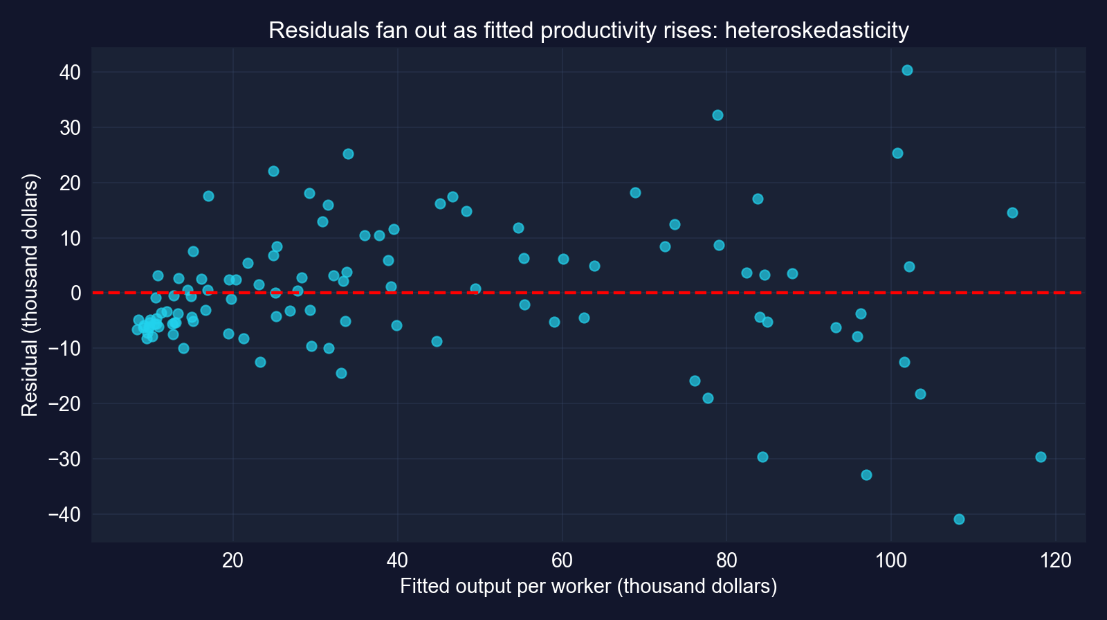
Residuals fan out: residual SD is $6,822 for the lower half of fitted values and $15,795 for the upper half. Poor countries also cluster below the line, a sign the straight line misses some curvature.

This is the residual plot that Task 5(c) asks for; the chapter’s code does not draw it, so it is computed here. Two patterns: a clear funnel (spread more than doubles from low to high fitted values), and a run of negative residuals among the poorest countries, which suggests the relationship is not linear in levels. Both are reasons why the classical SE is unreliable; the second also suggests a log specification, which later chapters use.

Task 4 code: does the slope differ by income group?

# continues from the previous block
threshold = data_2014["productivity"].median()             # the chapter's split
high_income = data_2014[data_2014["productivity"] > threshold].copy()
developing = data_2014[data_2014["productivity"] <= threshold].copy()
robust_high = pf.feols("productivity ~ capital", data=high_income, vcov="HC1")
robust_dev = pf.feols("productivity ~ capital", data=developing, vcov="HC1")
for name, res in [("High-income", robust_high), ("Developing", robust_dev)]:
    b, se = res.coef()["capital"], res.se()["capital"]
    t_05 = (b - 0.5) / se; dfx = int(res._N) - len(res.coef())   # test beta2 = 0.5
    print(name, int(res._N), b, se, res.tstat()["capital"], t_05, 2 * stats.t.sf(abs(t_05), dfx))

↗ Try it in Colab

Task 4 (more independent): split the sample at median productivity, estimate the regression in each half with robust SEs, test β2 = 0.5 in each group. This is the chapter’s own code. Watch the first line: the split is on the outcome, which matters for interpretation (two slides ahead).

Task 4 output: a flatter slope among high-productivity countries

Group	N	Slope	Robust SE	\(t\)	95% CI	\(t\) for \(\beta_2 = 0.5\)	\(R^2\)
High productivity	54	0.1541	0.0172	8.97	[0.1196, 0.1886]	−20.13	0.680
Low productivity	54	0.2059	0.0209	9.84	[0.1639, 0.2479]	−14.06	0.722
Full sample	108	0.1995	0.0111	17.94	[0.1774, 0.2215]	−27.03	0.870

HC1 SEs · split at median productivity, $32,781 · df = 52 in each half · all \(p < 0.001\)

Both slopes are significant and both are far below 0.5. Taken at face value, capital goes with less extra output in richer countries, consistent with diminishing returns.

The chapter’s table. Both group slopes reject zero and reject 0.5. The two intervals overlap only slightly (0.164 to 0.189). The chapter offers two readings in Key Concept 7.9: complementarity (rich countries’ slope higher) or diminishing returns (developing countries’ slope higher); the data point to the second. But the next slide shows that the way the sample was split biases this comparison.

Caveat: splitting on the outcome distorts the slopes

Group slopes with HC1 95% CIs. Rows marked * split the sample on capital instead of productivity.

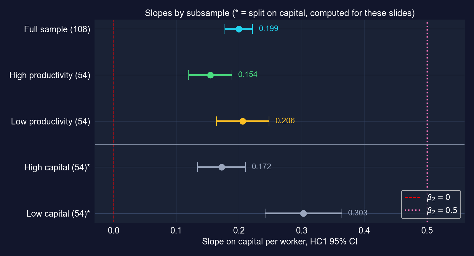
Split on capital*	Slope	Robust SE
High capital (54)	0.1720	0.0190
Low capital (54)	0.3026	0.0305

* computed for these slides · split at median capital, $108,046

Selecting on \(y\) truncates the outcome within each group and flattens both slopes. Splitting on \(x\) avoids that, and the low-capital slope comes out about 47% steeper than the chapter’s 0.206.

Why: within the “high productivity” group, every country has y above 32,781 by construction, so countries with high capital but unluckily low output are excluded; the same happens in reverse in the other group. That truncation pushes both slopes toward zero. Splitting on the regressor does not truncate the outcome, so it is the standard way to compare slopes across groups. Same estimator, same SEs, only the split variable changes. The diminishing-returns reading survives (0.303 vs 0.172), and the gap is larger. Still an association, not a causal marginal product.

Task 5: one picture of the full analysis

Productivity against capital per worker, coloured by the chapter’s median-productivity split, with the full-sample OLS line.

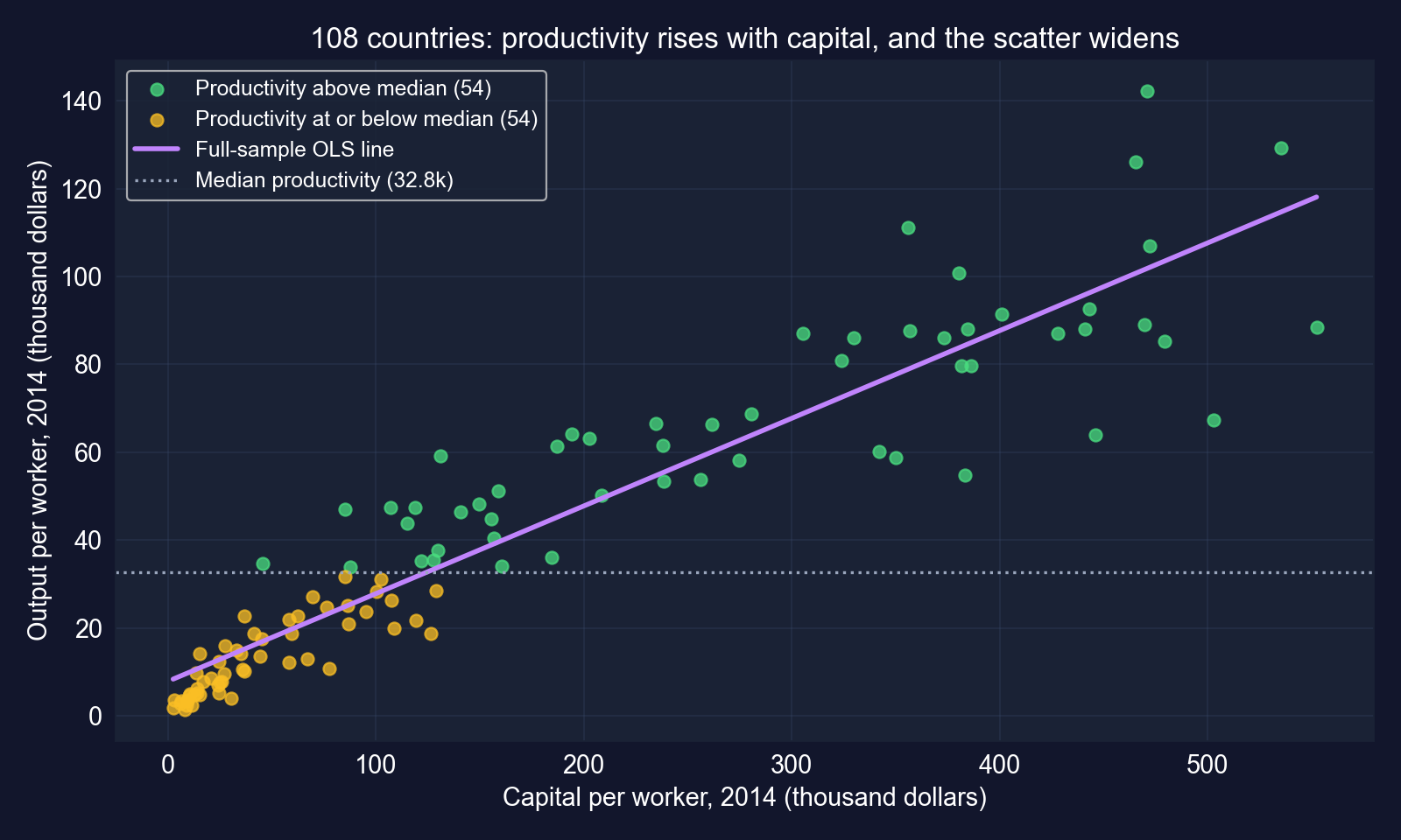
The picture shows everything the tables said: a strong positive slope, a widening scatter (heteroskedasticity) and a split that slices the cloud horizontally, along \(y\).

Task 5 asks for (a) a scatter with groups and the regression line, (b) a coefficient plot and (c) a residual plot. All three are on the last four slides: this scatter, the coefficient plot, and the residual plot. Notice how the dotted median line cuts the cloud horizontally: that is the selection-on-the-outcome problem made visible.

Task 5 code: the diagnostic plot the chapter leaves open

# continues from the previous block (model_convergence already fitted)
import matplotlib.pyplot as plt              # plotting
import numpy as np                           # array handling
fitted = model_convergence.predict()         # fitted productivity
resid = model_convergence.resid()            # residuals
plt.scatter(fitted, resid, alpha=0.7)        # residuals vs fitted (Task 5c)
plt.axhline(0, color="red", linestyle="--"); plt.xlabel("Fitted"); plt.ylabel("Residual"); plt.show()
low = fitted <= np.median(fitted)            # split by fitted value, not by y
print(np.std(resid[low], ddof=1), np.std(resid[~low], ddof=1))   # residual SD by half

↗ Try it in Colab

Output: residual SD $6,822 (lower half of fitted values) vs $15,795 (upper half), the numbers behind the fan shape shown under Task 3.

Task 5(c) in the chapter has no code; this block fills it in with the chapter’s methods only (a residual plot, plus a two-group SD comparison). The chapter’s own Task 5 code draws the two scatter panels and the coefficient plot; those plots are reproduced as the slide figures.

Task 6: the research summary, with the real numbers

Using a 2014 cross-section of 108 countries, I estimate the association between output per worker and physical capital per worker. Each additional $1,000 of capital per worker is associated with $199 more output per worker (HC1 robust SE = 0.011, \(t = 17.9\), \(p < 0.001\); 95% CI [0.177, 0.222]); capital explains 87% of the cross-country variation. The robust SE is 48% larger than the classical one, and residuals fan out with fitted productivity, so only robust inference is reported. The slope is far below the 0.5 benchmark (\(t = -27.0\)). Splitting the sample by capital per worker, the slope is 0.30 among capital-poor countries and 0.17 among capital-rich ones, consistent with diminishing returns. These are associations: capital moves with technology, human capital and institutions, and a levels regression does not test convergence.

A good summary reports magnitude, robust precision, the tests that matter and the limits of the design, in that order.

Task 6 asks for a 200–300 word summary covering question, data and methods, findings, inference, economic interpretation and limitations. This version uses only numbers verified for these slides; the capital-split slopes are labelled as computed for the slides in the deck. Students should write their own; this is a model of the structure.

Scorecard: Case Study 1

Question	Answer
Is it precise?	robust SE 0.0111; CI [0.177, 0.222]
Is it real?	robust \(t = 17.94\): reject \(\beta_2 = 0\)
Which values are plausible?	not 0.5 (\(t = -27.0\)); below 0.30 (\(p < 0.001\), one-sided)
Does it matter?	one SD of capital ↔︎ $31,576 output per worker (77% of the mean)
Is the SE honest?	no with classical SEs: robust SE is 48% larger; residuals fan out

Same toolkit as the houses, opposite lesson on the fourth row: here the robust SE is not optional.

Contrast with the house scorecard: there, classical and robust SEs agreed within 1.4%; here they differ by 48%. In both cases the coefficient is identical under either SE choice; what changes is how much we may claim to know.

Case Study 2 · Do nighttime lights track development in Bolivia?

DS4Bolivia · 339 municipalities · Tasks 1–6

Case Study 2 returns to the DS4Bolivia project from Chapter 1: can satellite nighttime lights tell us how developed a municipality is? Chapter 7 asks whether that association is statistically significant and how precisely it is estimated.

The question: is the light–development association real, and how big?

Research question. Across Bolivia’s municipalities, is the association between nighttime lights and development statistically significant, and how precisely can we estimate it?

\[\text{imds}_i = \beta_1 + \beta_2\,\ln(\text{NTL per capita})_i + u_i\]

• imds: Municipal Sustainable Development Index, 0–100
• ln_NTLpc2017: log of nighttime lights per capita, 2017
• 339 municipalities in 9 departments; 333 have both variables

Because \(x\) is in logs, \(\beta_2\) is the change in IMDS points when lights per capita are multiplied by \(e \approx 2.72\); doubling lights adds \(\beta_2 \ln 2 \approx 0.69\,\beta_2\) points.

A level-log model: the outcome is in index points, the regressor in logs. A one-unit increase in log NTL means lights per capita are 2.72 times higher, a 172% increase, as the chapter’s Task 6 notes. Doubling lights is a 0.693 increase in the log. Six municipalities lack the lights variable and drop out of the regression.

Code: load the DS4Bolivia data

!pip install -q pyfixest                     # pyfixest is not preinstalled in Colab
import pandas as pd, pyfixest as pf          # data and OLS
from scipy import stats                      # t-distribution for manual tests
url_bol = "https://raw.githubusercontent.com/quarcs-lab/ds4bolivia/master/ds4bolivia_v20250523.csv"
bol = pd.read_csv(url_bol)                   # 339 municipalities, 351 columns
bol_key = bol[["mun", "dep", "imds", "ln_NTLpc2017"]].copy()   # keep what we need
reg_data = bol_key[["imds", "ln_NTLpc2017"]].dropna()          # complete cases only
print(f"Total municipalities: {len(bol_key)}")
print(f"Complete cases for regression: {len(reg_data)}")
reg_data.describe().round(3)                 # summary statistics

↗ Try it in Colab

Self-contained: the first block of Case Study 2. dropna() keeps the 333 municipalities with both variables. Always report how many observations a regression loses to missing data.

Output: 333 municipalities, a wide spread of development

Variable	Mean	SD	Min	Max
imds (0–100)	51.16	6.76	35.70	80.20
ln_NTLpc2017	13.88	1.18	9.06	17.06

N = 333 complete cases out of 339 municipalities

IMDS spans 44.5 points; log lights span 8 units, which means lights per capita differ by a factor of about 3,000 between the dimmest and the brightest municipality.

exp(17.06 − 9.06) = exp(8.0) ≈ 2,980. The range of IMDS, 35.7 to 80.2, is the yardstick the chapter uses for economic significance in Task 6. Note that the dimmest municipalities in terms of log lights are not all the least developed: the relationship is noisy.

Task 1 code: estimate and test the slope

# continues from the previous block (reg_data already built)
model = pf.feols("imds ~ ln_NTLpc2017", data=reg_data)   # classical SEs
model.summary()                                          # full table
t_stat = model.tstat()["ln_NTLpc2017"]                   # t for H0: beta2 = 0
p_value = model.pvalue()["ln_NTLpc2017"]                 # two-sided p-value
print(model.coef()["ln_NTLpc2017"], model.se()["ln_NTLpc2017"], t_stat, p_value)
print("Reject H0" if p_value < 0.05 else "Fail to reject H0")
print(model._r2)                                         # R-squared

↗ Try it in Colab

Task 1 (guided): OLS of IMDS on log lights, extract t and p, test H0: β2 = 0 at 5%.

Task 1 output: 3.4 IMDS points per log unit of light

Variable	Coef.	SE	\(t\)	\(p\)
Intercept	4.377	3.544	1.24	0.218
ln_NTLpc2017	3.370	0.254	13.25	< 0.001

N = 333 · classical SEs · \(R^2 = 0.347\)

Reject \(H_0: \beta_2 = 0\): \(t = 13.25\).

IMDS against log lights per capita, with the OLS line.

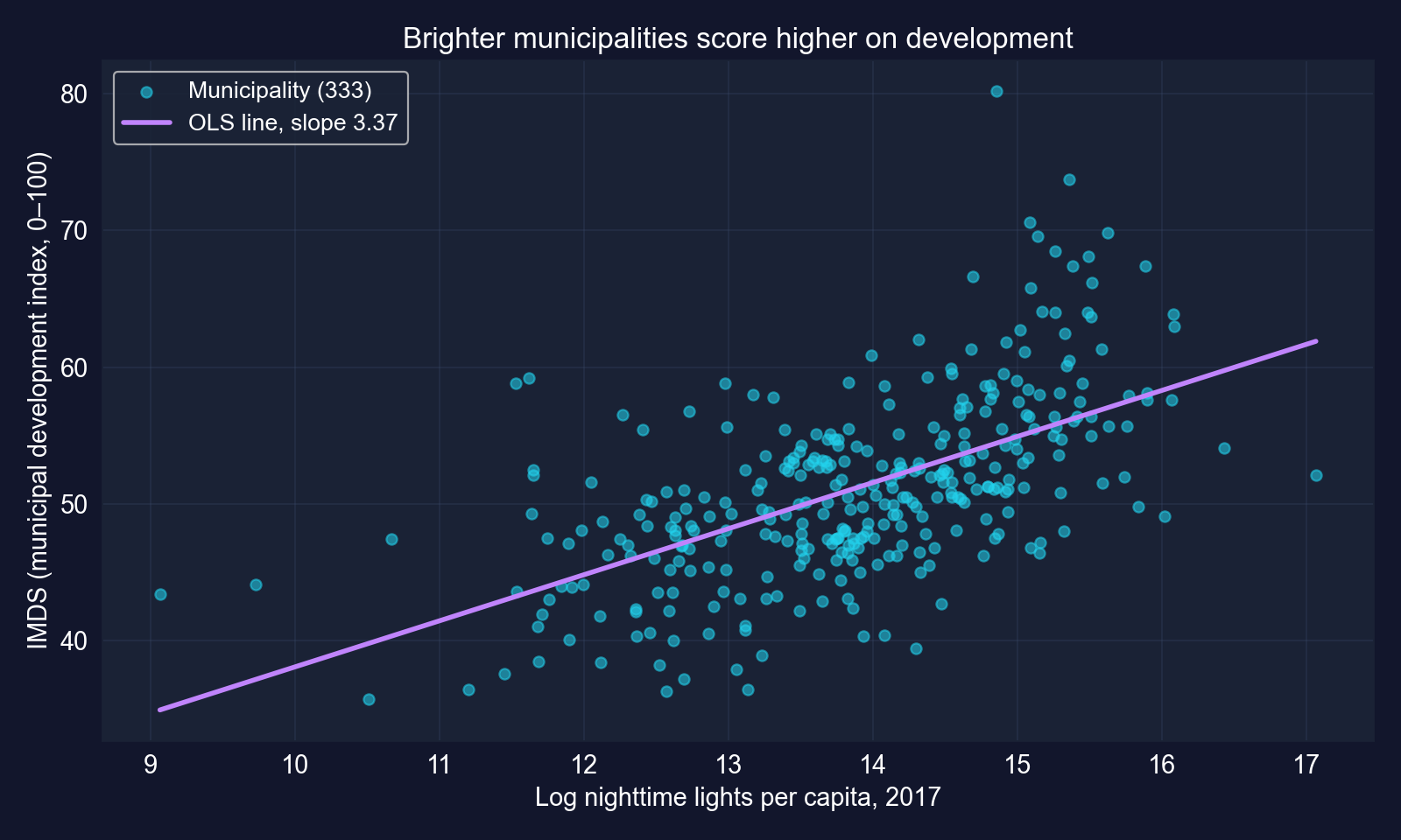
Brighter municipalities are measurably more developed, but lights explain only 35% of the variation in IMDS.

The slope is 13 standard errors from zero. The intercept is the predicted IMDS at log lights = 0, far outside the data (minimum 9.06), and is not interpretable; its insignificance is irrelevant. R² = 0.347 leaves 65% of the variation to other factors, which is why the chapter later adds satellite embeddings in multiple regression.

Task 2: a 95% confidence interval for the slope

# continues from the previous block (model already fitted)
ci = model.confint()                                     # 95% CIs, classical SEs
ci_lower = ci.loc["ln_NTLpc2017"].iloc[0]                # lower bound
ci_upper = ci.loc["ln_NTLpc2017"].iloc[1]                # upper bound
print(ci_lower, ci_upper, ci_lower <= 0 <= ci_upper)     # does it contain zero?

↗ Try it in Colab

Point estimate	95% CI	Contains 0?
3.370	[2.87, 3.87]	no

Correct reading: intervals built this way capture the true slope 95% of the time, and this one runs from 2.87 to 3.87 IMDS points per log unit of light. Zero is far outside it.

Task 2 (guided). The chapter’s prompt suggests “we are 95% confident that…”, a common shorthand; the precise reading is about the procedure (Section 7.3). The interval is narrow relative to the estimate because n = 333 and log lights vary a lot.

Task 3 code: robust standard errors

# continues from the previous block
model_robust = pf.feols("imds ~ ln_NTLpc2017", data=reg_data, vcov="HC1")   # HC1 SEs
se_d, se_r = model.se()["ln_NTLpc2017"], model_robust.se()["ln_NTLpc2017"]
print(se_d, se_r, se_r / se_d)                           # SE ratio robust / default
print(model.tstat()["ln_NTLpc2017"], model_robust.tstat()["ln_NTLpc2017"])
print(model_robust.confint().loc["ln_NTLpc2017"])        # robust 95% CI
print(model_robust.se()["Intercept"], model_robust.pvalue()["Intercept"])

↗ Try it in Colab

Task 3 (semi-guided): compare default and HC1 standard errors, and discuss why robust SEs matter for municipality-level data. The chapter prints the SE ratio; the robust CI and the intercept line are added for these slides.

Task 3 output: the robust SE is 18% larger

Variable	Coef.	Default SE	Robust SE	Ratio	Robust \(t\)	Robust 95% CI
Intercept	4.377	3.544	4.135	1.167	1.06	[−3.76, 12.51]
ln_NTLpc2017	3.370	0.254	0.299	1.175	11.27	[2.78, 3.96]

N = 333 · HC1 SEs · robust \(p < 0.001\) for the slope, 0.291 for the intercept

Residuals against fitted IMDS (computed for these slides).

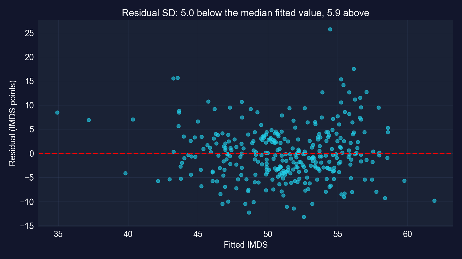
Moderate heteroskedasticity: the slope’s SE rises 17.5% and \(t\) falls from 13.25 to 11.27. Every conclusion survives; use the robust numbers from here on.

Following the chapter’s thresholds, a 17.5% difference sits between “small” (under 10%) and “must use robust” (over 20%); the chapter’s best practice is to report robust SEs regardless. The residual plot shows a slightly wider spread above the median fitted value (residual SD 5.9 vs 5.0). A standard caveat not covered in Chapter 7: municipalities in the same department may share shocks (spatial correlation), which HC1 does not address; cluster-robust SEs, introduced later in the book, would.

Task 4: is the slope exactly 5?

# continues from the previous block (model_robust already fitted)
beta_hat = model_robust.coef()["ln_NTLpc2017"]           # 3.370
se_robust = model_robust.se()["ln_NTLpc2017"]            # robust SE
df = int(model_robust._N) - len(model_robust.coef())     # 333 - 2 = 331
t_manual = (beta_hat - 5) / se_robust                    # H0: beta2 = 5
p_two_sided = 2 * stats.t.sf(abs(t_manual), df=df)       # two-sided p-value
print(t_manual, df, p_two_sided)

↗ Try it in Colab

\(H_0\)	\(t\)	df	\(p\)	Decision
\(\beta_2 = 5\)	−5.45	331	\(9.8\times 10^{-8}\)	reject

A slope of 5 is ruled out: it lies well above the robust interval [2.78, 3.96]. The test and the interval tell the same story.

Task 4 (semi-guided), using robust SEs as the chapter instructs. stats.t.sf is the survival function, 1 − cdf, so 2 × sf(|t|) is the two-sided p-value. With classical SEs (computed for these slides) the test gives t = −6.41, an even stronger rejection. The CI–test duality from 7.5 applies with robust SEs too: 5 is outside the robust interval, so it is rejected at 5%.

Task 5: is the association positive?

# continues from the previous block
t_onesided = model_robust.tstat()["ln_NTLpc2017"]        # robust t for H0: beta2 = 0
p_onesided = stats.t.sf(t_onesided, df=df)               # right tail: Ha beta2 > 0
print(t_onesided, p_onesided)

↗ Try it in Colab

\(H_0\)	\(H_a\)	Robust \(t\)	One-sided \(p\)	Decision
\(\beta_2 \le 0\)	\(\beta_2 > 0\)	11.27	\(1.8\times 10^{-25}\)	reject

Overwhelming evidence of a positive association. A one-sided test is legitimate here because the direction was stated before estimation, and the estimate points that way.

Task 5 (independent). The one-sided p-value is half the two-sided one because the estimate has the predicted sign (Section 7.6). “Strong evidence for a positive relationship” is a statement about association: the chapter’s Task 6 asks students to discuss whether significance proves causation, and it does not.

Task 6 code: put the magnitude in context

# continues from the previous block
imds_range = reg_data["imds"].max() - reg_data["imds"].min()   # 44.5 points
imds_std = reg_data["imds"].std()                               # 6.76 points
beta = model_robust.coef()["ln_NTLpc2017"]                      # 3.370
print(beta, 100 * beta / imds_range, 100 * beta / imds_std)     # per log unit
print(beta * 0.693, 100 * beta * 0.693 / imds_range)            # doubling lights
ci_r = model_robust.confint().loc["ln_NTLpc2017"]               # robust CI
print(ci_r.iloc[0] * 0.693, ci_r.iloc[1] * 0.693)               # CI for doubling
sd_x = reg_data["ln_NTLpc2017"].std()                           # 1.18 log units
print(beta * sd_x, beta * sd_x / imds_std, model._r2)           # one-SD contrast, R²

↗ Try it in Colab

Task 6 (independent) asks for a discussion of statistical vs practical significance. The chapter’s code computes the range, the SD and the doubling effect; the CI for the doubling effect and the one-SD contrast are added for these slides.

Task 6 output: significant beyond doubt, modest in size

Comparison	IMDS change	Relative to
+1 log unit of lights (×2.72)	3.37	7.6% of the IMDS range; 50% of its SD
Doubling lights (+0.693)	2.34	5.2% of the range · robust CI [1.93, 2.74]
+1 SD of log lights (1.18)	3.98	0.59 SD of IMDS

Range = 44.5 points, SD = 6.76 · CI for doubling and one-SD row computed for these slides · \(R^2 = 0.347\)

• Significant at 1%, 5% and 10%: robust \(p < 0.001\)
• Practically: doubling a municipality’s lights goes with about 2.3 more IMDS points, a modest step on a 0–100 scale
• Not causal: urbanization, electrification, roads and market access drive both lights and development

Statistical significance here is beyond doubt; economic significance is moderate; causality is not established. Three different questions, three different answers.

Key Concept 7.13 uses a hypothetical effect of 5 points (11% of the range); the actual estimate is 3.37, or 7.6% of the range. Doubling lights is a large change, yet it predicts only about 2.3 points. Policy reading: a programme that “doubles lights” would not by itself transform development; lights are a proxy for economic activity, not a lever. Omitted variables are the main threat to any causal reading.

Scorecard: Case Study 2

Question	Answer
Is it precise?	robust SE 0.299; CI [2.78, 3.96]
Is it real?	robust \(t = 11.27\): reject \(\beta_2 = 0\); positive one-sided, \(p < 0.001\)
Which values are plausible?	not 5 (\(t = -5.45\))
Does it matter?	doubling lights ↔︎ +2.3 IMDS points (5.2% of the range): moderate
Is the SE honest?	robust SE 17.5% larger: report it; department-level correlation not yet addressed

Same five rows, a third pattern: precise and real, but modest, and the SE still has a caveat (spatial correlation) that HC1 cannot fix.

Across the three datasets the coefficient never changes with the SE choice, but the honest uncertainty does: +1.4% for the houses, +48% for the countries, +17.5% for the municipalities. The next part compares them side by side.

Reading it right

Act III · Synthesis

Act III pulls the three datasets together, confronts the most common misreadings, and lists what to carry forward to multiple regression.

Three datasets, one toolkit

	Houses (7.1–7.7)	Countries (Case 1)	Municipalities (Case 2)
N	29	108	333
Slope \(b_2\)	73.771	0.1995	3.370
Classical SE	11.175	0.0075	0.254
Robust (HC1) SE	11.330	0.0111	0.299
Robust / classical	1.014	1.484	1.175
Robust \(t\)	6.51	17.94	11.27
Robust 95% CI	[50.52, 97.02]	[0.1774, 0.2215]	[2.78, 3.96]
\(R^2\)	0.617	0.870	0.347

Every slope is highly significant, yet the SE correction ranges from 1% to 48%. Whether heteroskedasticity matters is an empirical question, so the robust SE should be the default.

The highest R² (countries) comes with the largest heteroskedasticity problem, which shows that fit and honest uncertainty are separate questions. The smallest sample (houses) has the least heteroskedasticity. None of the verdicts on β2 = 0 change, but in all three the classical SE would have misstated precision by between 1% and 48%.

Seven misreadings to avoid

1. “95% chance \(\beta_2\) is in the interval”: no, 95% of intervals cover \(\beta_2\)
2. “\(p < 0.001\), so the effect is large”: \(p\) measures evidence against \(H_0\), not size
3. “We fail to reject, so \(\beta_2 = 90\)”: the data are also consistent with 60 and 95
4. “Halve the \(p\)-value for any one-sided test”: only when the estimate points toward \(H_a\)
5. “Robust SEs only when a test finds heteroskedasticity”: use them by default
6. “Split the sample by the outcome to compare slopes”: that truncates \(y\) and biases both slopes
7. “Significant, so causal”: every slope in this deck is an association

Each one is a real trap, and each has a slide in this deck that shows the correct reading with the chapter’s own numbers.

1: Section 7.3 and the coverage simulation. 2: Section 7.4 and Task 6 of Case 2. 3: Section 7.5. 4: Section 7.6; the previous version of this deck halved the p-value for the wrong tail. 5: Section 7.7. 6: Case Study 1, Task 4. 7: all three examples, especially the nighttime-lights case.

The tempting shortcut, and the correction

Objection. “\(t = 17.9\), \(p < 0.001\), \(R^2 = 0.87\): capital clearly drives productivity, and we know the effect to the third decimal.”

Response. The classical SE overstated precision by 48%, the residuals fan out and curve, the sample split biased the group slopes, and nothing in a cross-section of levels identifies a causal effect. Significance tells you the association is not noise. It does not tell you how big it is, how precise it truly is, or why it exists.

Read every regression table with four questions: how big, how precise (with an honest SE), how plausible are the alternatives, and what would make it causal.

Steelman the objection: the association really is strong and robust to the SE choice. But every adjective in the objection overreaches: “drives” is causal, “know to the third decimal” ignores the 48% understatement of uncertainty. Chapters 10–13 add controls, and Chapter 13 adds research designs, precisely because significance cannot answer the “why”.

What to carry forward

• \(t = (b_2 - \beta_2^{*})/\operatorname{se}(b_2) \sim T(n-2)\): every test is “estimate minus claim, in SE units”
• A 95% CI is \(b_2 \pm t_{n-2,\,0.025}\,\operatorname{se}(b_2)\) and contains every value a two-sided 5% test does not reject
• \(\operatorname{se}(b_2)\) shrinks with a tighter fit, more data (\(1/\sqrt n\)) and more spread in \(x\)
• One-sided tests: the claim goes in \(H_a\), the direction is fixed in advance, halving needs the right sign
• Cross-sections: vcov="HC1" by default; look at the residuals; a large gap signals a model problem
• Always report magnitude and precision; significance is not importance, and association is not causation

The chapter’s key takeaways, sharpened by what the deck verified: the HC0 vs HC1 distinction, the conditions for halving a p-value, the 1%–48% range of robust corrections across datasets, and the selection-on-the-outcome caveat. Next: multiple regression (Chapters 10–11), where the same t-statistic and confidence interval apply to each coefficient, and joint tests extend them to several coefficients at once.

Estimate, then measure your doubt honestly: a range and a test, not just a number.