Why percentages, not dollars?
Act I · The tension
Economists care about proportionate change
A $10,000 raise means very different things at a $30,000 salary and at a $300,000 salary.
So the number we usually want is a percentage, not a dollar amount — a return to education, a price elasticity, a growth rate. The natural logarithm is the one transformation that turns a regression slope directly into that percentage.
Where we’re going
- One property of \(\ln\) that makes it the workhorse of econometrics
- Semi-elasticity vs elasticity — the two ways \(y\) can respond to \(x\)
- Four functional forms (level, log-linear, log-log, linear-log) and how each slope is read
- Earnings & education — the same data, four interpretations, with
pyfixest - Exponential growth — logs linearize it, and the Rule of 72 reads off a doubling time
Five ideas anchor this chapter
- Natural log \(\ln\) — inverse of \(e^x\); turns multiplicative differences into additive ones
- Key approximation — \(\Delta \ln(x) \approx \Delta x / x\), so \(100 \times \Delta\ln(x) \approx \%\Delta x\)
- Semi-elasticity — \(\%\Delta y\) per one-unit change in \(x\) (log-linear slope)
- Elasticity — \(\%\Delta y\) per 1% change in \(x\) (log-log slope), unit-free
- Compound growth — \(x_t = x_0(1+r)^t\) is a straight line once you log it
Logs let a single regression slope be read as a percentage — that is the whole point.
From logs to elasticities
Act II · The investigation
The one log property that matters: \(\Delta \ln(x) \approx \Delta x / x\)
For small changes, the change in \(\ln(x)\) is the proportionate change in \(x\) — multiply by 100 to get a percent.
import numpy as np                           # numpy → logs, exponentials, arrays

x0, x1 = 40, 40.4                            # x rises from 40 to 40.4 (a 1% increase)

exact  = (x1 - x0) / x0                      # exact proportionate change = 0.010000
approx = np.log(x1) - np.log(x0)             # log approximation Δln(x)   = 0.009950
print(f"exact proportionate change: {exact:.6f}  ({exact*100:.2f}%)")
print(f"log approximation Δln(x):   {approx:.6f}  ({approx*100:.2f}%)")
print(f"difference: {abs(exact-approx):.6f}") # tiny — the approximation is excellent for small movesTwo responses: semi-elasticity vs elasticity
- Semi-elasticity \(= \dfrac{\Delta y / y}{\Delta x}\) — a one-unit move in \(x\) (e.g. one more year of school) → a percentage move in \(y\). Estimated by a log-linear slope.
- Elasticity \(= \dfrac{\Delta y / y}{\Delta x / x}\) — a 1% move in \(x\) → a percentage move in \(y\). Unit-free. Estimated by a log-log slope.
| Form | Model | Slope \(\beta_1\) reads as |
|---|---|---|
| Linear | \(y = \beta_0 + \beta_1 x\) | \(\Delta y\) in units per unit of \(x\) |
| Log-linear | \(\ln y = \beta_0 + \beta_1 x\) | \(100\beta_1 \approx \%\Delta y\) per unit of \(x\) |
| Log-log | \(\ln y = \beta_0 + \beta_1 \ln x\) | $_1 = $ elasticity (% per %) |
| Linear-log | \(y = \beta_0 + \beta_1 \ln x\) | \(\beta_1/100 = \Delta y\) per 1% of \(x\) |
Our question: how do earnings vary with education?
171 full-time women workers aged 30 (2010). Earnings are right-skewed (mean $41,413, median $36,000, max $172,000), so the log scale pulls in the long tail. We take logs and fit all four forms with pyfixest.
!pip install -q pyfixest                     # pyfixest is NOT preinstalled in Colab (-q = quiet)

import pandas as pd                          # tabular data
import numpy as np                           # np.log for the transforms
import pyfixest as pf                        # OLS with R-style formulas

url = "https://raw.githubusercontent.com/quarcs-lab/data-open/master/AED/AED_EARNINGS.DTA"
data = pd.read_stata(url)                    # 171 women aged 30: earnings, education
data["lnearn"] = np.log(data["earnings"])    # log of the outcome
data["lneduc"] = np.log(data["education"].astype(float))   # log of the regressor (int8 → float first)

m_lin    = pf.feols("earnings ~ education", data=data)   # 1. linear:      $ per year
m_loglin = pf.feols("lnearn ~ education",   data=data)   # 2. log-linear:  semi-elasticity
m_loglog = pf.feols("lnearn ~ lneduc",      data=data)   # 3. log-log:     elasticity
m_linlog = pf.feols("earnings ~ lneduc",    data=data)   # 4. linear-log:  $ per 1%

print(100 * m_loglin.coef()["education"])    # 13.1 → ~13.1% more earnings per extra year
m_loglin.summary() # β0, β1, SE, t, p, R²Same data, four fitted lines — four different questions
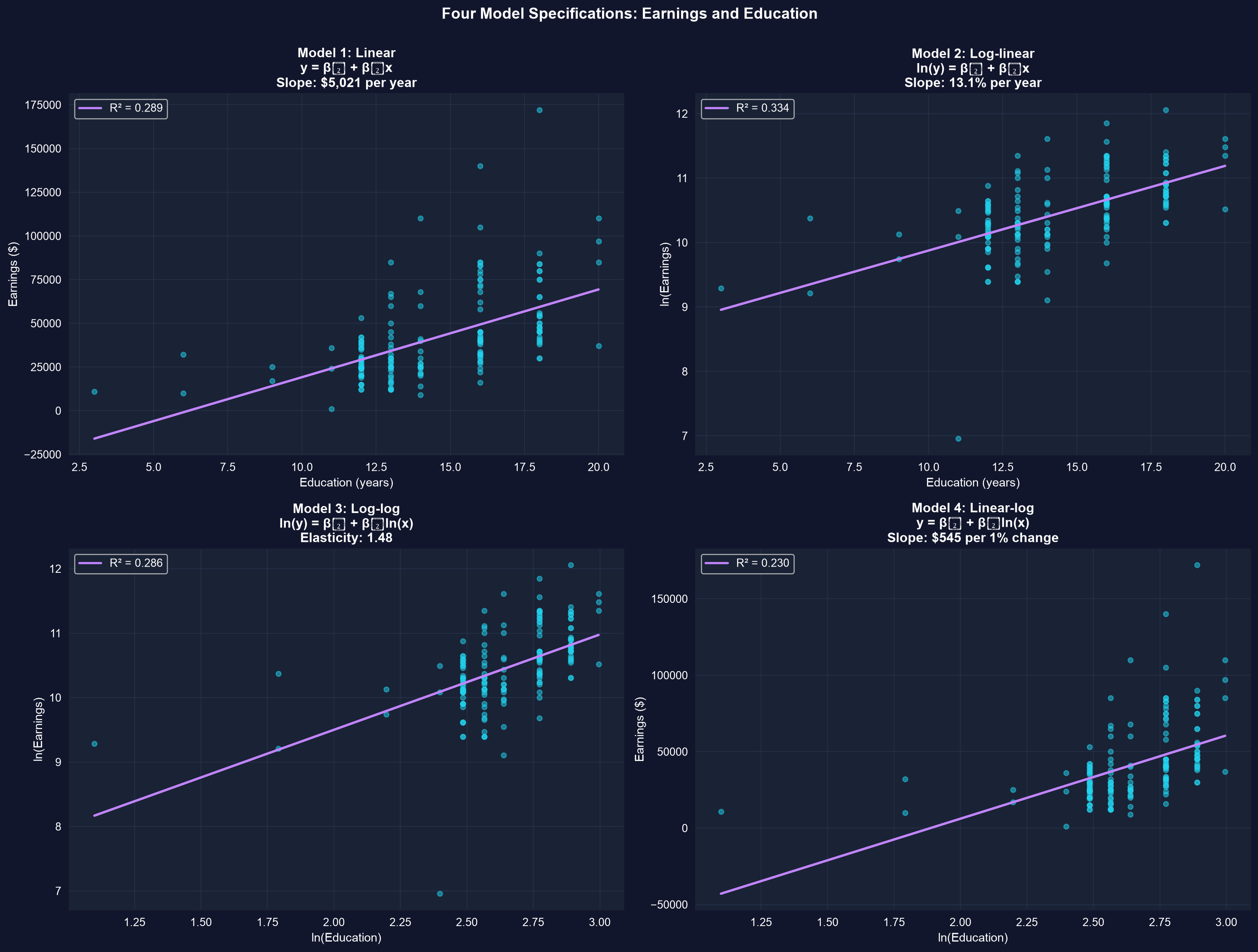
Each panel fits one specification. The log transforms straighten the curvature the linear model misses.
Log-linear fits best among the \(\ln\)(earnings) models (R² = 0.334); logging only \(x\) bends the line into diminishing returns.
Reading the four slopes
- Linear: $5,021 more earnings per extra year — a fixed dollar amount (implausible at the top end).
- Log-linear: about 13.1% more earnings per extra year — the semi-elasticity, and the usual choice.
- Log-log: elasticity 1.48 — a 1% rise in education is associated with ~1.48% higher earnings.
- Linear-log: about $545 more earnings per 1% of education — dollars from a percentage move.
Compare \(R^2\) only across models with the same dependent variable — not across level and log outcomes.
Exponential growth becomes a straight line in logs
\(x_t = x_0(1+r)^t\) curves upward in levels, but \(\ln(x_t) = \ln(x_0) + \ln(1+r)\,t \approx \ln(x_0) + r\,t\) is linear — so the slope of \(\ln x\) on time estimates \(\ln(1+r) \approx r\); the exact rate is \(e^{\text{slope}} - 1\).
!pip install -q pyfixest                     # self-contained cell: install pyfixest (quiet)

import pandas as pd                          # tabular data
import numpy as np                           # np.exp for the exact growth rate
import pyfixest as pf                        # OLS with R-style formulas

url = "https://raw.githubusercontent.com/quarcs-lab/data-open/master/AED/AED_SP500INDEX.DTA"
data = pd.read_stata(url)                    # S&P 500 index, 1927–2019 (lnsp500 precomputed)

fit = pf.feols("lnsp500 ~ year", data=data)  # slope = ln(1+r) ≈ growth rate r
r = fit.coef()["year"]                       # ≈ 0.0653
print(f"log slope: {100*r:.2f}% per year")   # ≈ 6.53% (log approximation)
print(f"exact growth: {100*(np.exp(r)-1):.2f}% per year")   # ≈ 6.75% per year
print(f"Rule of 72: doubles every {72/(100*r):.0f} years") # ≈ 11 yearsLogs turn a curve into a slope you can read
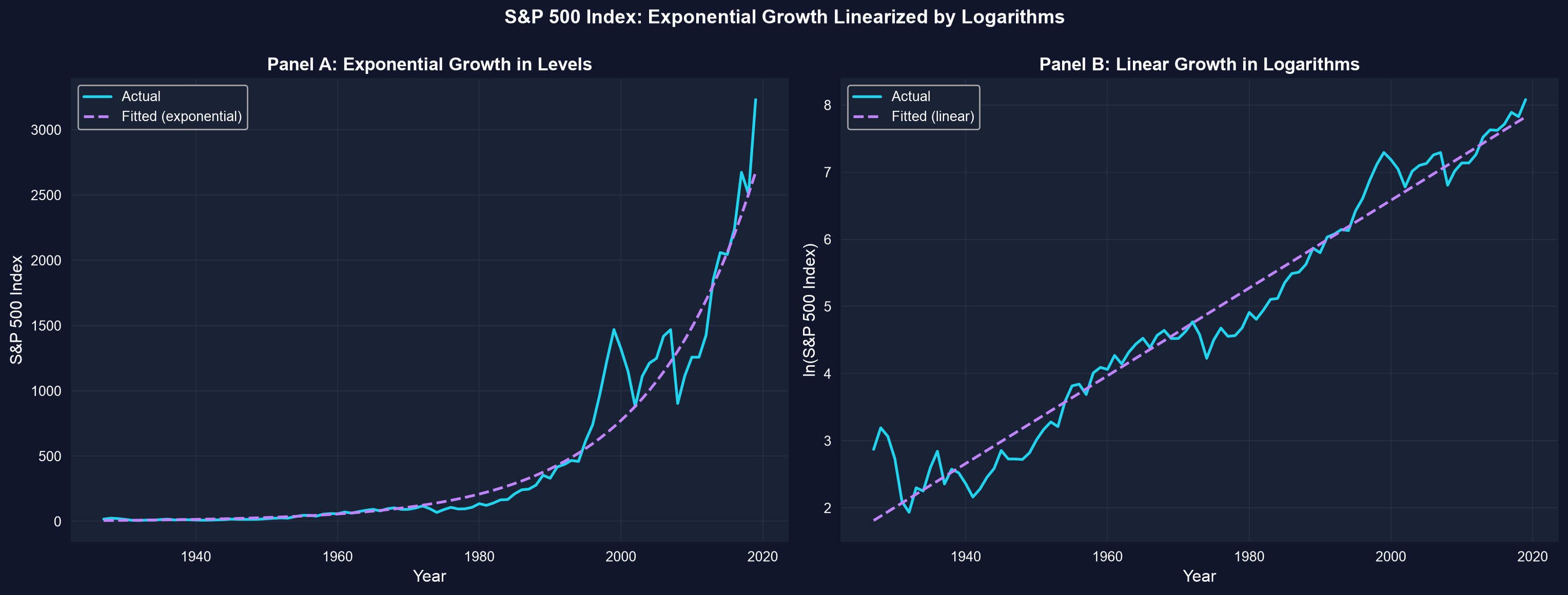
The same S&P 500 series: an exponential curve in levels (left), a near-straight line in logs (right).
Log slope 0.065 → exact growth of about 6.75% per year over 1927–2019 → the index doubles about every 11 years (Rule of 72).
Reading it right
Act III · The resolution
The approximation has limits — and logs have a domain
Objection. “The log-linear slope is 0.131, so the return to a year of education is exactly 13.1%.”
Response. \(100\beta_1\) is an approximation that holds for small coefficients. At \(\beta_1 = 0.131\) the exact effect is \(100\,(e^{0.131}-1) \approx 14.0\%\) — close, but not identical. And \(\ln\) is undefined at zero or negative values, so logs only apply to strictly positive variables.
Report the exact \(100(e^{\beta_1}-1)\) once \(|\beta_1|\) clears about 0.10; never log a variable that can be zero.
What to carry forward
- \(\Delta\ln(x) \approx \Delta x/x\): a log change is a proportionate change (for small moves).
- Log-linear → semi-elasticity (\(100\beta_1 \approx \%\Delta y\) per unit); log-log → elasticity (% per %).
- Choose the form from economic theory + data + interpretation — log-linear is the common default.
- Exponential growth is linear in logs: regress \(\ln x\) on time; the slope estimates \(\ln(1+r) \approx r\) (exact: \(e^{\text{slope}} - 1\)).
- Treat finite percentage effects as approximations (\(100(e^{\beta_1}-1)\) is exact); logs need positive data.