The question

Act I · The tension

One cause at a time is a fantasy

House prices depend on size and bedrooms and age and lot size — all at once.

A bivariate regression of price on bedrooms alone says each bedroom is worth $23,667. But bigger houses also have more bedrooms. How much is the bedroom really worth, once we hold size fixed? Multiple regression is the tool that separates tangled effects.

The headline tension: observational data mixes many causes. Multiple regression is how we isolate the partial effect of one variable while controlling for the rest.

Where we’re going

• Look first — scatterplot matrix and correlations before any model
• Estimate a multiple regression by OLS with pyfixest
• Interpret each slope as a partial effect — holding the others constant
• Compare models with \(R^2\) vs adjusted \(R^2\) (and AIC/BIC)
• Diagnose confounding and perfect collinearity

Six ideas anchor this chapter

• Multiple regression — \(\hat{y} = b_1 + b_2 x_2 + \cdots + b_k x_k\); each slope is a partial effect
• Correlation matrix — every pairwise \(r\) at a glance, before modeling
• Control variable — added to keep a confounder from biasing the focal slope
• Confounder — drives both \(x\) and \(y\), faking a relationship if omitted
• Adjusted \(R^2\) — \(R^2\) with a penalty for extra regressors
• Perfect collinearity — one regressor is an exact combination of others → inestimable

A multiple-regression slope answers “all else equal” — the question economics actually asks.

From one variable to many

Act II · The investigation

The bedrooms coefficient is a trap

29 house sales in Davis, California (1999), with size, bedrooms, bathrooms, lot size, age, month sold.

\[\widehat{\text{price}} = b_1 + b_2\,\text{size} + b_3\,\text{bedrooms} + \cdots + b_7\,\text{monthsold}\]

On its own, bedrooms looks like a $23,667 driver. The suspicion: that number is really size showing up in disguise. To find out, we first look at how the variables move together.

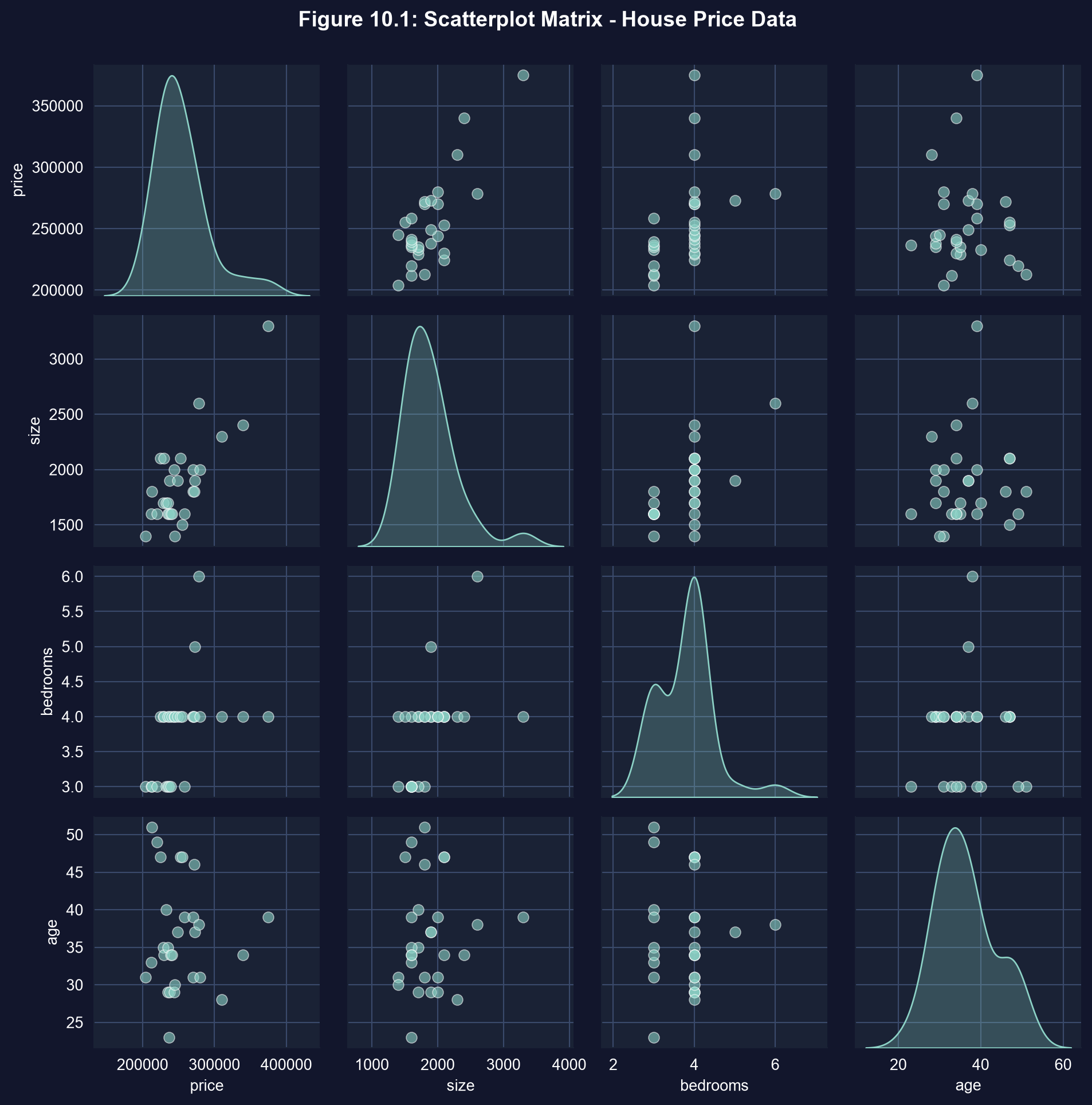
Step 1 — see every pair at once with a scatterplot matrix

import pandas as pd                          # tabular data
import seaborn as sns                        # statistical visualization

url = "https://raw.githubusercontent.com/quarcs-lab/data-open/master/AED/AED_HOUSE.DTA"
data = pd.read_stata(url)                    # 29 Davis, CA house sales

plot_vars = ["price", "size", "bedrooms", "age"]   # columns to cross-plot
g = sns.pairplot(data[plot_vars],            # every two-way scatter + KDE on the diagonal
                 diag_kind="kde",
                 plot_kws={"color": "#1fb2dd"})     # brand cyan markers

↗ Try it in Colab

A scatterplot matrix is pure exploratory data analysis — it reveals linear associations, nonlinearities, clusters, and outliers before any formal modeling.

Every pair, in one view

Each off-diagonal panel is one two-way scatter; the diagonal shows each variable’s distribution. Price climbs with size most clearly.

Look before you model: the matrix shows which predictors move with price — and with each other.

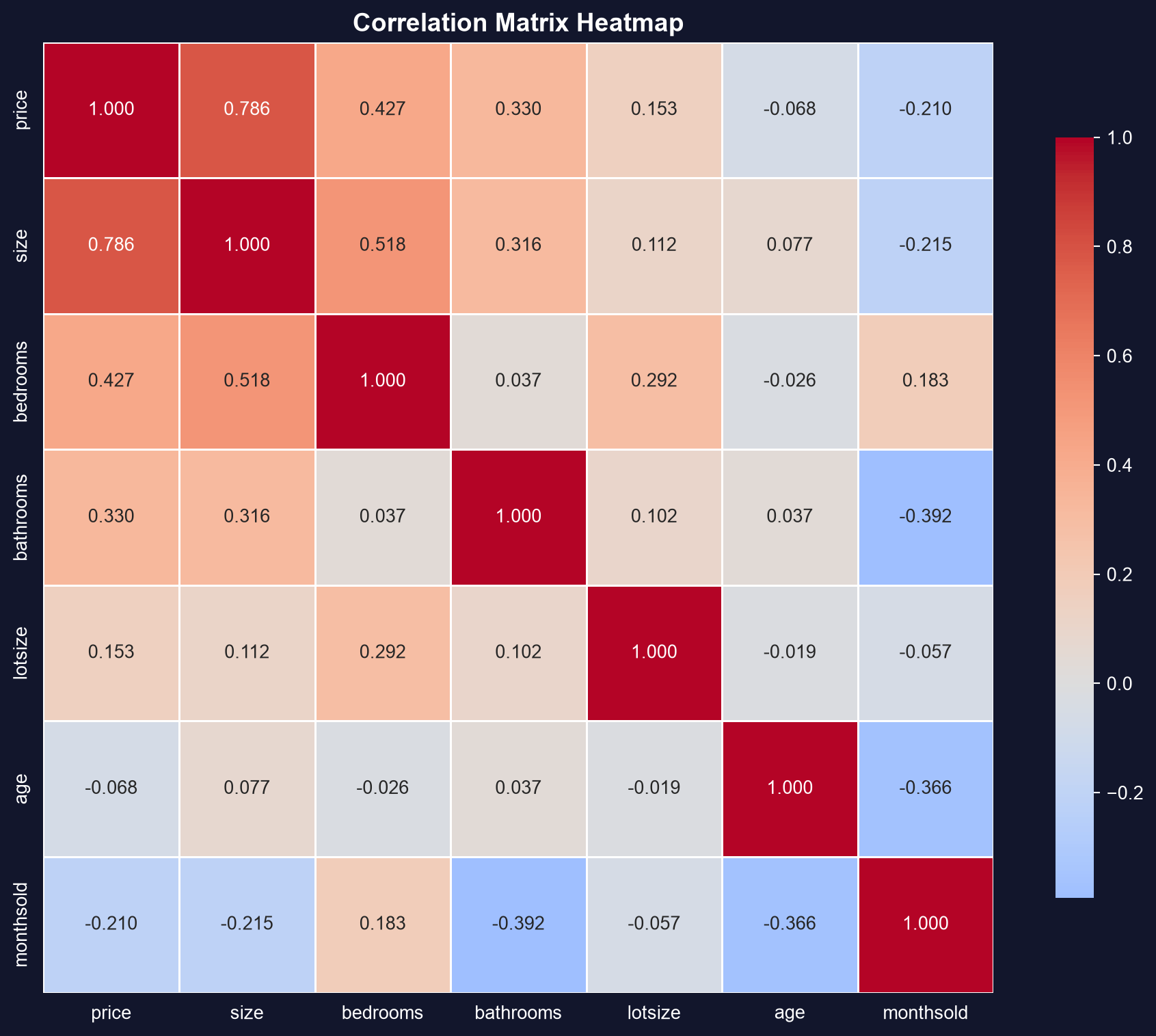
Step 2 — quantify the pairwise links with a correlation matrix

import pandas as pd                          # tabular data
import seaborn as sns                        # heatmap

url = "https://raw.githubusercontent.com/quarcs-lab/data-open/master/AED/AED_HOUSE.DTA"
data = pd.read_stata(url)                    # load the 29 house sales

corr_vars = ["price", "size", "bedrooms", "bathrooms", "lotsize", "age"]
corr = data[corr_vars].corr()               # pandas .corr() → pairwise correlation matrix

sns.heatmap(corr, annot=True, fmt=".2f",     # print each r in its cell
            cmap="coolwarm", center=0)        # diverging colours around 0
corr                                          # show the raw matrix too

↗ Try it in Colab

Size is the strongest predictor — and it moves with bedrooms

Correlation heatmap of the six variables. Price–size is the hottest cell; size–bedrooms is warm.

\(r(\text{price},\text{size}) = 0.79\) · \(r(\text{price},\text{bedrooms}) = 0.43\) · \(r(\text{size},\text{bedrooms}) = 0.52\) — size and bedrooms overlap, so their effects will be hard to separate.

Step 3 — fit the full multiple regression with pyfixest

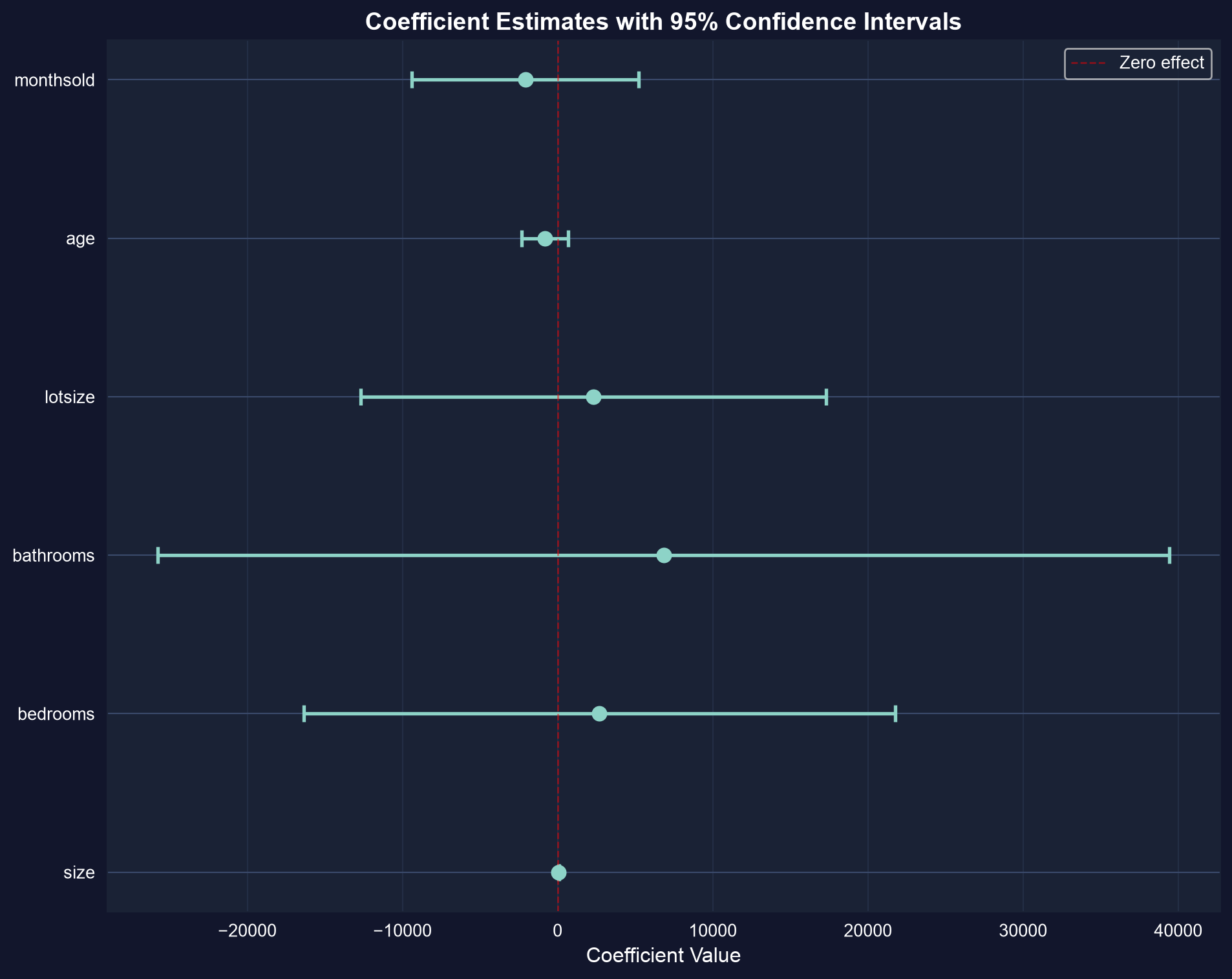
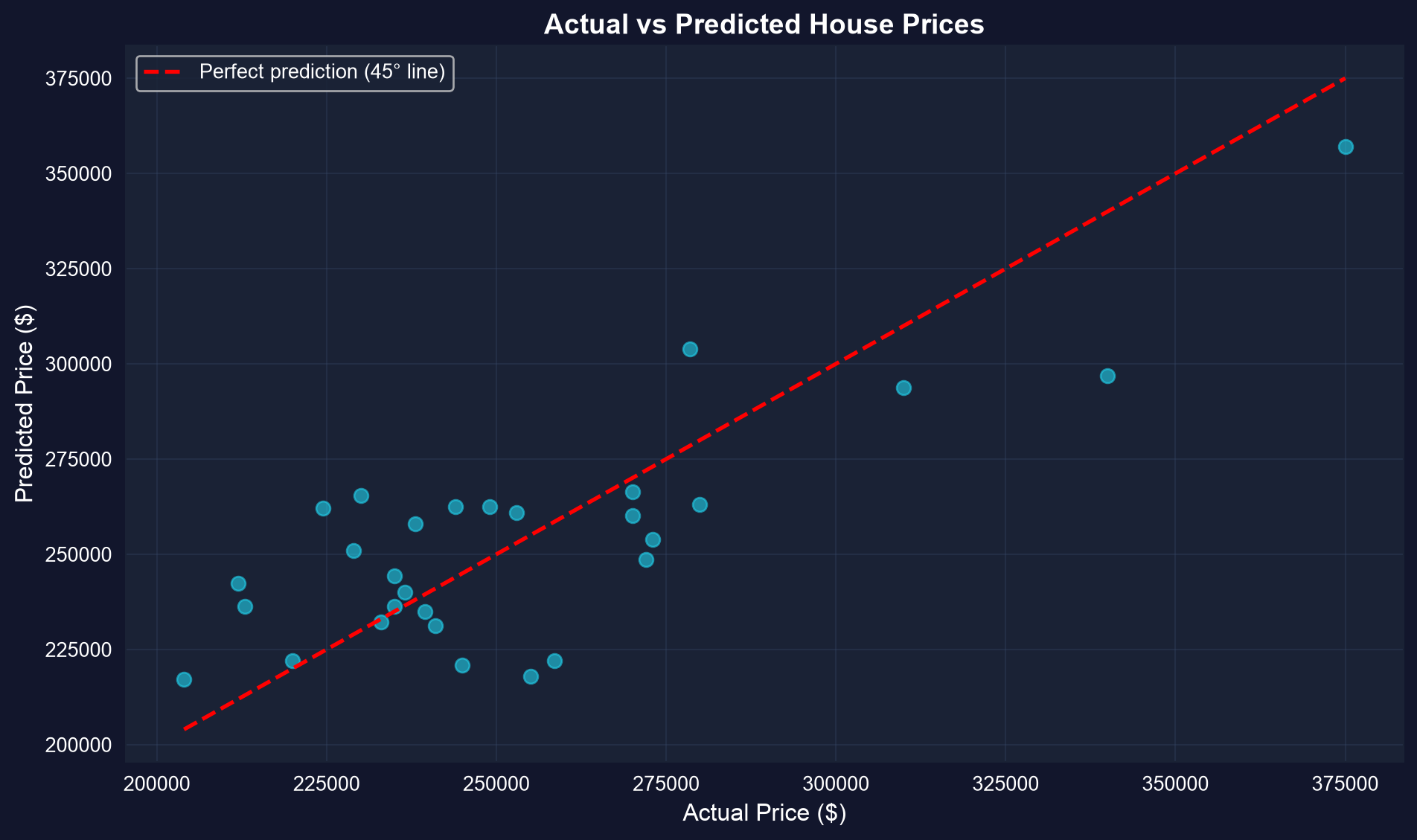
!pip install -q pyfixest                     # install pyfixest in Colab (-q = quiet; not preinstalled)

import pandas as pd                          # tabular data
import pyfixest as pf                         # pyfixest → OLS regression, R-style formulas

url = "https://raw.githubusercontent.com/quarcs-lab/data-open/master/AED/AED_HOUSE.DTA"
data = pd.read_stata(url)                    # load the 29 Davis, CA house sales

fit = pf.feols("price ~ size + bedrooms + bathrooms + lotsize + age + monthsold",
               data=data)                    # OLS with six regressors at once
fit.summary()                                # partial slopes, SEs, t, p, R²

↗ Try it in Colab

feols takes an R-style formula; adding predictors with + is all it takes to go from bivariate to multiple. Classical SEs here (AED switches to robust SEs in Chapter 12).

Only size clears the bar — once everything is controlled

Coefficient estimates with 95% confidence intervals. Only size’s interval excludes zero.

size \(= \$68.37\)/sq ft, \(t = 4.44\), \(p < 0.001\) (95% CI ≈ $36–$100). Every other interval straddles zero.

Controlling for size unmasks the bedroom

• Bedrooms alone: $23,667 per bedroom — impressive, and misleading.
• Bedrooms + size: the bedrooms slope collapses to $1,553.
• Most of the “bedrooms effect” was really size: bigger houses have more bedrooms and cost more.
• size is a textbook confounder of bedrooms — and adding it as a control fixes the estimate.

A partial effect is the honest number: what one extra bedroom adds, holding size fixed.

The FWL theorem: a partial effect is a bivariate slope on residuals

import pandas as pd
import pyfixest as pf                                 # pyfixest OLS

data = pd.read_stata("https://raw.githubusercontent.com/quarcs-lab/data-open/master/AED/AED_HOUSE.DTA")

# Step 1 — strip out the part of size explained by the other regressors
others = pf.feols("size ~ bedrooms + bathrooms + lotsize + age + monthsold", data=data)
data["resid_size"] = others._u_hat                    # residualized size (size "net of" the rest)

# Step 2 — regress price on residualized size alone
pf.feols("price ~ resid_size", data=data).coef()      # → 68.37, exactly the full-model size slope

↗ Try it in Colab

Frisch–Waugh–Lovell: the multiple-regression slope on size equals the bivariate slope of price on the part of size that is independent of the other regressors. That residual variation is exactly what a partial effect uses.

More variables never lower \(R^2\) — adjusted \(R^2\) can fall

Actual vs. predicted price for the full model: points track the 45° line, but scatter remains.

Simple (size only): \(R^2 = 0.617\), \(\bar{R}^2 = 0.603\). Full (six regressors): \(R^2 = 0.651\) but \(\bar{R}^2\) falls to \(0.555\).

Choosing between models

• Plain \(R^2\) can never go down when you add regressors — it rewards clutter.
• Adjusted \(R^2\) divides by degrees of freedom, so junk predictors push it down.
• AIC / BIC penalize complexity harder still; smaller is better, BIC favors parsimony.
• On \(n = 29\) houses, the five extra predictors barely earn their keep — the simple model is competitive.

With few observations, parsimony wins: don’t buy a lower \(\bar{R}^2\) with variables that add nothing.

Reading it right

Act III · The resolution

When a coefficient simply cannot exist

Objection. “If more predictors help, why not add size_twice = 2 × size?”

Response. Perfect collinearity. size_twice carries zero new information, so OLS has no unique solution — the software drops one of the pair (pyfixest warns which). Like identical twins with one set of measurements: distinct names, identical data. Watch for it whenever one regressor is an exact combination of others.

Correlation among regressors is normal; an exact linear dependence is fatal to estimation.

What to carry forward

• Each multiple-regression slope is a partial effect — the change in \(y\) per unit of \(x_j\), others held fixed.
• Look before you model: scatterplot matrix (sns.pairplot) + correlation matrix (.corr()).
• Omitting a confounder biases the focal slope; adding it as a control corrects it ($23,667 → $1,553).
• Compare specifications with adjusted \(R^2\), AIC, and BIC — not plain \(R^2\).
• Perfect collinearity makes a model inestimable; moderate correlation just widens standard errors.

Hold the others constant — then the slope tells the truth.