The question
Act I · The tension
Six variables compete to explain house prices
We regress the price of 29 Davis, CA houses on size, bedrooms, bathrooms, lotsize, age, and months-on-market.
\[\text{price} = \beta_1 + \beta_2\,\text{size} + \beta_3\,\text{bedrooms} + \cdots + \beta_7\,\text{monthsold} + u\]
Every coefficient comes back non-zero. But a point estimate is not evidence — which of these effects could just be sampling noise? Inference is how we tell signal from luck.
Where we’re going
- Estimate the full model and read its coefficients, SEs, and \(t\)-statistics
- Quantify precision — why \(se(b_j)\) shrinks with fit and variation, and inflates with multicollinearity
- Build confidence intervals \(b_j \pm t_{n-k,\,0.025}\,se(b_j)\) for each effect
- Test one coefficient at a time with a \(t\)-test, and groups of coefficients with an \(F\)-test
- Present results professionally — robust SEs, significance stars, parsimony
Six ideas anchor this chapter
- \(t\)-statistic for \(b_j\) — standardized distance from a hypothesized value, distributed \(T(n-k)\)
- Degrees of freedom \(n-k\) — the data’s “budget” left after estimating \(k\) parameters (\(29-7=22\) here)
- Standard error \(se(b_j)\) — shrinks with good fit and unique variation; balloons under multicollinearity
- Overall \(F\)-test — does the model collectively explain \(y\)? (\(H_0:\beta_2=\cdots=\beta_k=0\))
- Restricted vs. unrestricted — compare \(\text{RSS}\) to test a group of variables jointly
- Significance stars —
******flag the 10%, 5%, 1% thresholds at a glance
Each extra parameter costs a degree of freedom — in a sample of 29, that cost is real.
From estimates to evidence
Act II · The investigation
Fit the full model — size dominates, the rest are quiet
!pip install -q pyfixest                     # pyfixest isn't preinstalled in Colab (-q = quiet)

import pandas as pd                          # tabular data
import pyfixest as pf                         # OLS with R-style formulas

url = "https://raw.githubusercontent.com/quarcs-lab/data-open/master/AED/AED_HOUSE.DTA"
data = pd.read_stata(url)                    # 29 Davis, CA house sales (1999)

fit = pf.feols("price ~ size + bedrooms + bathrooms + lotsize + age + monthsold",
               data=data)                    # multiple regression, intercept auto-added

fit.summary() # coefficients, SEs, t, p for all 7 parametersOnly size clears the bar — at \(\$68.37\) per square foot
- size: \(\$68.37\)/sq ft, \(t = 4.44\), \(p = 0.0002\) — highly significant, holding all else constant
- bedrooms \(\$2{,}685\) (\(p=0.77\)), bathrooms \(\$6{,}833\) (\(p=0.67\)), age \(-\$833\) (\(p=0.26\)) — none significant
- \(R^2 = 0.651\) — the model explains 65% of price variation, but adjusted \(R^2 = 0.555\)
Non-zero is not the same as significant: five of six slopes could plausibly be zero.
Precision has a formula — and multicollinearity is its enemy
\[se(b_j) = \frac{s_e}{\sqrt{\sum_i \widetilde{x}_{ji}^2}}, \qquad \widetilde{x}_{ji} = x_j \text{ residualized on all other regressors}\]
\(se(b_j)\) shrinks when the model fits well (\(s_e\) small) and when \(x_j\) carries variation the other regressors don’t. Because bigger houses tend to have more bedrooms (\(r = 0.52\)), residualization strips out about 42% of the variation in bedrooms — inflating its SE.
With \(n=29\) and correlated predictors, estimates are imprecise by construction — the data are stretched thin.
A confidence interval is the plausible range for each effect
import pandas as pd                          # tabular data
import pyfixest as pf                         # estimation
from scipy import stats                       # t critical value

url = "https://raw.githubusercontent.com/quarcs-lab/data-open/master/AED/AED_HOUSE.DTA"
data = pd.read_stata(url)                    # load the 29 houses

fit = pf.feols("price ~ size + bedrooms + bathrooms + lotsize + age + monthsold", data=data)

fit.confint()                                # 95% CI: b_j ± t(n-k, 0.025) · se(b_j)
t_crit = stats.t.ppf(0.975, df=29 - 7) # critical value from T(22) ≈ 2.074Only size’s interval misses zero
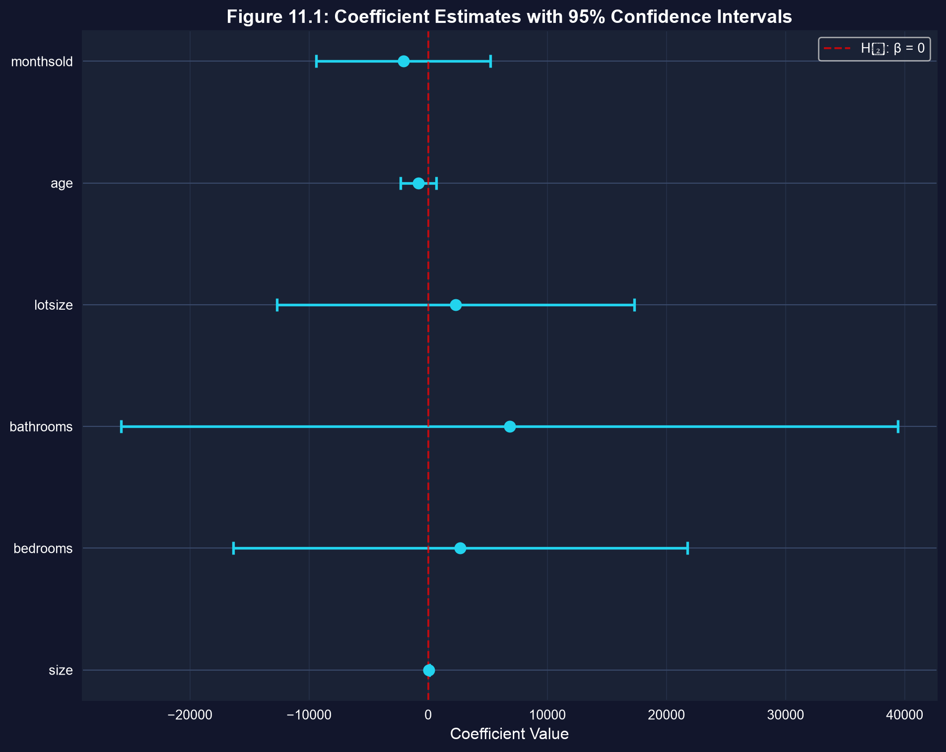
Each bar is a 95% confidence interval. size sits entirely above zero; every other interval straddles it.
size: \([\$36.45,\ \$100.29]\) — even the low end adds \(\$36\)/sq ft. An interval excluding zero is significance at 5%.
A \(t\)-test asks whether one coefficient equals a value
import numpy as np                           # arrays
# from the fitted model: b_size = 68.37, se_size = 15.39, df = 22

fit = pf.feols("price ~ size + bedrooms + bathrooms + lotsize + age + monthsold", data=data)

b, se = fit.coef()["size"], fit.se()["size"] # estimate and its standard error

t = (b - 50) / se                            # H0: beta_size = 50  →  t = (68.37 - 50)/15.39
p = 2 * (1 - stats.t.cdf(abs(t), df=29 - 7)) # two-sided p-value from T(22)

print(f"t = {t:.2f}, p = {p:.3f}") # t = 1.19, p = 0.245 → fail to rejectOne \(t\)-test can’t judge several variables at once
Testing bedrooms, bathrooms, lotsize, age, monthsold one by one ignores that they’re correlated — and inflates the chance of a false “significant.”
Instead, compare two models by their residual sum of squares:
\[F = \frac{(\text{RSS}_R - \text{RSS}_U)/q}{\text{RSS}_U/(n-k)} \sim F(q,\, n-k)\]
The restricted model drops the variables; the unrestricted keeps them. Does dropping them hurt the fit?
The \(F\)-test judges a group of variables together
import numpy as np                           # arrays
from scipy import stats                       # F distribution

full = pf.feols("price ~ size + bedrooms + bathrooms + lotsize + age + monthsold", data=data)
size_only = pf.feols("price ~ size", data=data)   # restricted: drop the other 5

rss_u, rss_r = np.sum(full._u_hat**2), np.sum(size_only._u_hat**2)
q, n_k = 5, 29 - 7                           # 5 restrictions, 22 residual df
F = ((rss_r - rss_u) / q) / (rss_u / n_k)    # joint F-statistic
p = 1 - stats.f.cdf(F, q, n_k)               # upper-tail p-value

print(f"F({q},{n_k}) = {F:.2f}, p = {p:.3f}") # F = 0.42, p = 0.832Two \(F\)-tests, two verdicts
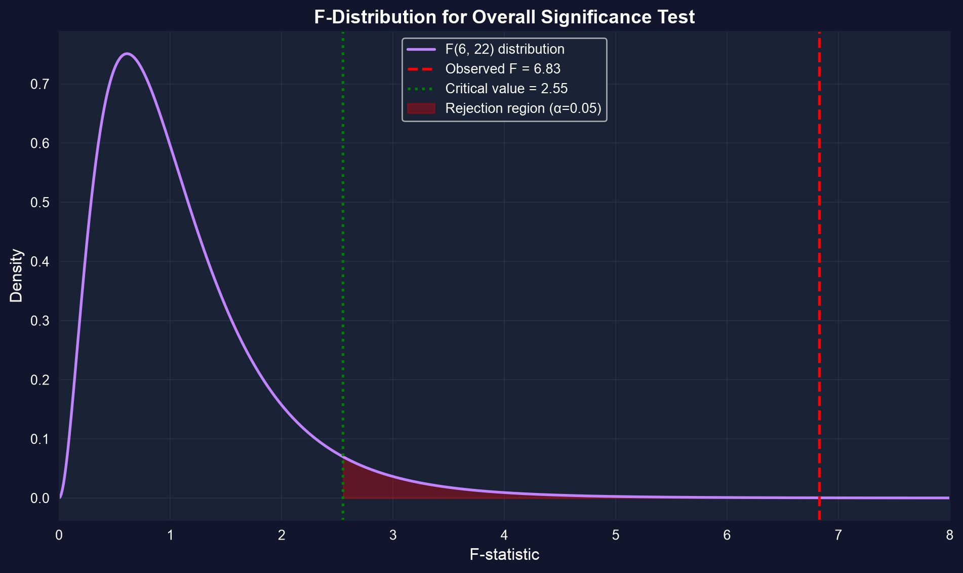
The \(F(q,\,n-k)\) distribution is right-skewed and positive; we reject in the far right tail.
- Overall: \(F(6,22) = 6.83\), \(p = 0.0003\) — the model collectively explains price. Reject.
- The five extras: \(F(5,22) = 0.42\), \(p = 0.832\) — jointly redundant beyond
size. Fail to reject.
The model works — but all of its work is being done by size alone.
Reading it right
Act III · The resolution
Report robust SEs and let stars carry the signal
Report size as \(68.37^{***}\) and the rest unstarred — a reader sees in one glance where the evidence lives. The robust SE for size barely moves (\(\$15.39 \to \$15.36\)); the others shift both ways (−26% for lot size to +23% for bathrooms), but no conclusion changes.
Simpler wins: parsimony beats a crowded model
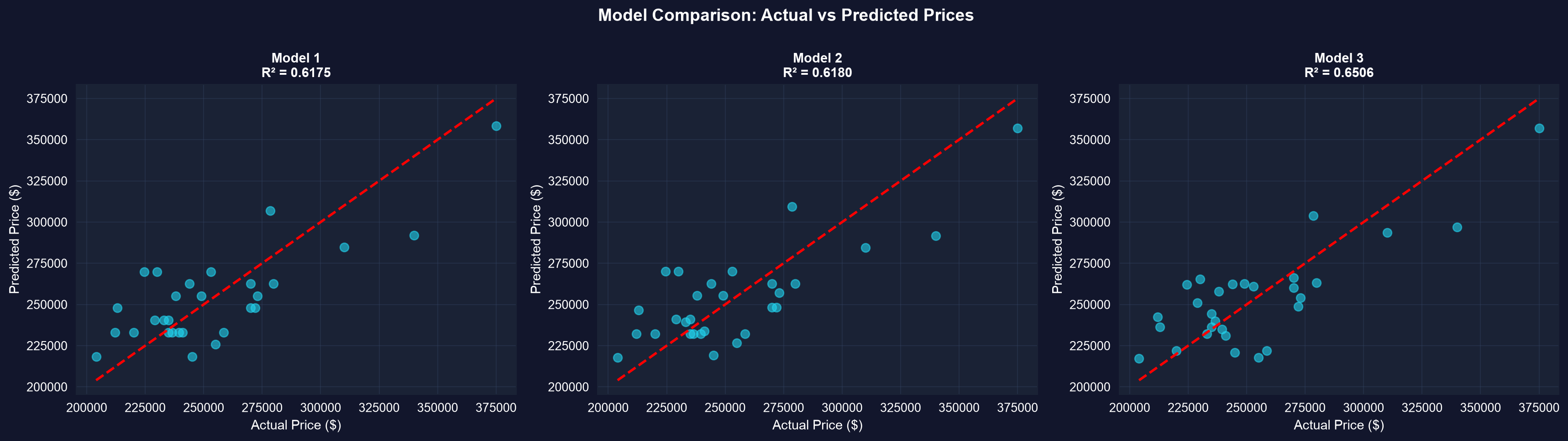
Actual vs. predicted price. The size-only model tracks the full model almost exactly.
- Size-only: \(R^2 = 0.617\), adjusted \(R^2 = 0.603\) — the highest adjusted \(R^2\)
- Full model: \(R^2 = 0.651\) but adjusted \(R^2 = 0.555\) — six extra parameters, net loss
\(R^2\) never falls with more variables; adjusted \(R^2\) charges for the complexity. Prefer the model that earns its parameters.
Keep two cautions in view
Objection. “The five variables are insignificant — so bedrooms and bathrooms don’t affect price.”
Response. Failing to reject is not accepting. With \(n = 29\) and predictors that move together, the data simply can’t resolve those effects — not that they’re zero. A larger, less collinear sample might.
Inference quantifies what this sample can support; small, correlated data support less than they seem to.
What to carry forward
- The \(t\)-statistic \(t = b_j/se(b_j)\) follows \(T(n-k)\); a CI excluding zero means significance at that level.
- \(se(b_j)\) falls with fit and unique variation, and rises with multicollinearity — the small-sample tax.
- Use an \(F\)-test for groups of coefficients: overall (\(H_0:\) all slopes \(=0\)) and subset (restricted vs. unrestricted).
- Report robust (HC1) SEs by default for cross-sectional data, with significance stars.
- Judge models on adjusted \(R^2\) and parsimony, not raw \(R^2\) — here,
sizealone is enough.