When the standard assumptions break

Act I · The tension

OLS gives the right line — but can lie about how sure we are

The classical standard-error formula assumes errors are independent and equally spread. Real data rarely cooperate: cross-sections are heteroskedastic, grouped data are clustered, time series are autocorrelated.

Under all three, OLS coefficients stay unbiased — the line is still right. What breaks is the standard error: the $t$-stats, $p$-values, and intervals built on it become untrustworthy. This chapter fixes the uncertainty, then asks what regression can and cannot predict.

Where we’re going

Repair the SEs — heteroskedastic-robust (HC1), cluster-robust, and HAC (Newey–West)
Predict honestly — the average outcome vs. one individual outcome
Know the floor — why individual forecasts stay wide no matter the sample size
Watch the sample — selection on $Y$ biases; selection on $X$ only costs precision
Judge estimators & tests — BLUE, the bootstrap, and the power of a test

Six ideas anchor this chapter

Robust SEs — HC1 for heteroskedasticity; coefficients unchanged, only SEs move
Cluster-robust SEs — errors correlated within groups, independent across them
Autocorrelation — one period’s error echoes into the next; fix with HAC SEs
CI for $E[Y\mid X^*]$ — the average outcome; shrinks to zero as $n\to\infty$
Prediction interval — one individual outcome; the “$1+$” floor never disappears
Power $=1-\beta$ — the chance a true effect is actually detected

Coefficients stay put; this chapter is about trusting the numbers around them.

Repairing the standard errors

Act II · The investigation

Three violations, three fixes — coefficients never change

Heteroskedasticity (error variance varies) — common in cross-sections → HC1 robust SEs
Clustered errors (correlated within groups) — panels, hierarchies → cluster-robust SEs
Autocorrelation (errors correlated over time) — time series → HAC (Newey–West) SEs

The OLS point estimate is unbiased under all three. Only the standard error needs the correction.

Robust SEs are one keyword: `vcov="HC1"`

!pip install -q pyfixest                     # pyfixest isn't preinstalled in Colab (-q = quiet)

import pandas as pd                          # tabular data
import pyfixest as pf                         # pyfixest → OLS with robust SEs, R-style formulas

url = "https://raw.githubusercontent.com/quarcs-lab/data-open/master/AED/AED_HOUSE.DTA"
data = pd.read_stata(url)                    # 29 Davis, CA house sales (1999)

f = "price ~ size + bedrooms + bathrooms + lotsize + age + monthsold"
default = pf.feols(f, data=data)             # classical SEs (assume homoskedasticity)

robust = pf.feols(f, data=data, vcov="HC1")  # SAME coefficients, heteroskedastic-robust SEs

↗ Try it in Colab

For these houses, robust SEs tell the same story

Each extra square foot is worth about $68 in sale price, and it is strongly significant either way: robust SE for size is 15.36 vs. default 15.39 ($p = 0.0002$).

The biggest adjustments are bathrooms (robust SE ~23% larger) and lotsize (~26% smaller) — but both stay far from significance under either method.

A rule of thumb: if robust SEs move more than ~30%, heteroskedasticity is real — report the robust ones.

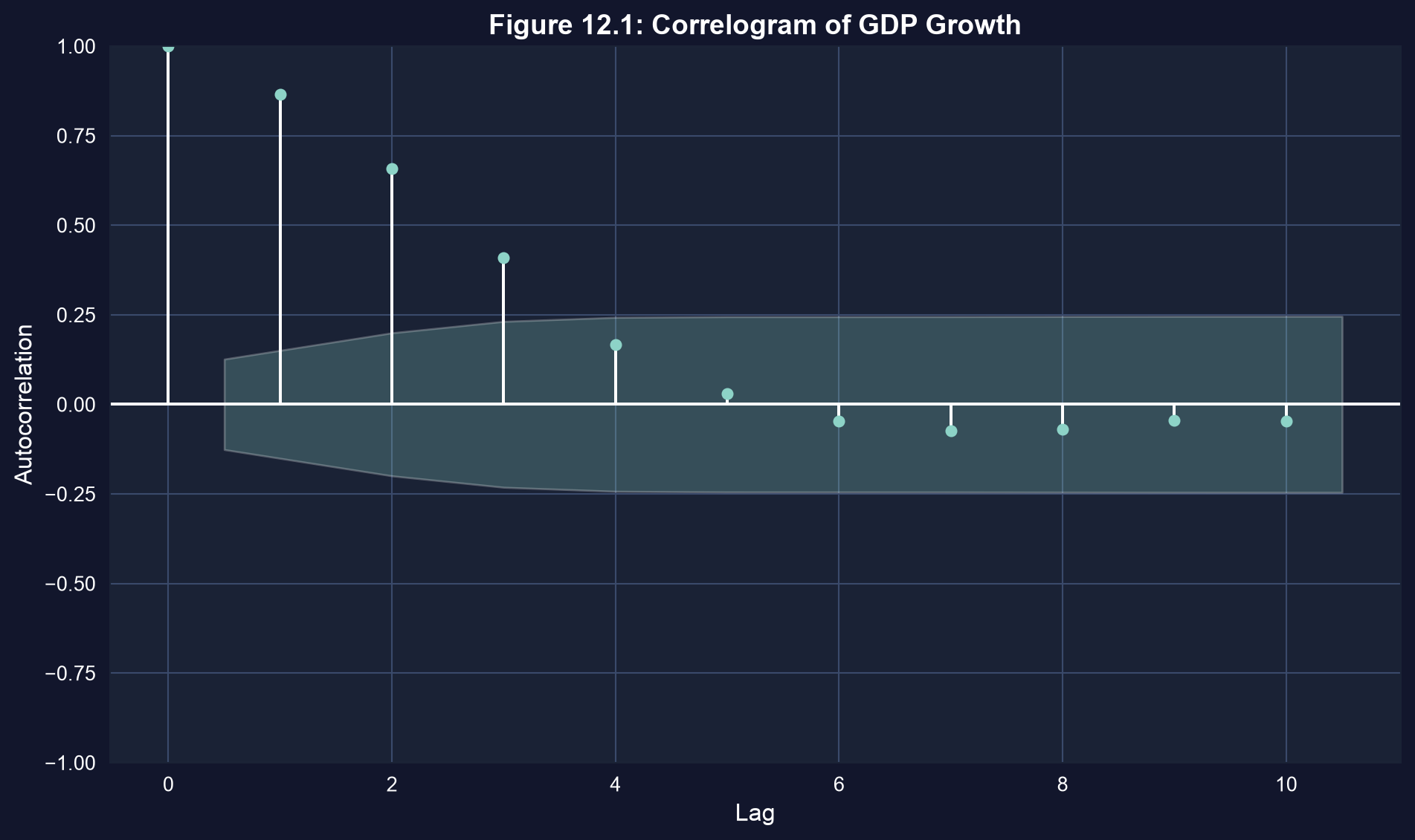
Time series carry an echo — the correlogram shows it

Correlogram of U.S. real GDP-per-capita growth (T = 241). Bars outside the shaded band are statistically significant; a positive lag-1 value means fast-growth quarters cluster (each value is a year-over-year rate, so neighbors overlap).

Positive autocorrelation means consecutive observations aren’t independent — so there is less information than the sample count suggests.

HAC (Newey–West) SEs account for that echo

import numpy as np                           # numerics
from statsmodels.regression.linear_model import OLS as smOLS  # for HAC covariance

url = "https://raw.githubusercontent.com/quarcs-lab/data-open/master/AED/AED_REALGDPPC.DTA"
growth = pd.read_stata(url)["growth"].dropna()   # real GDP-per-capita growth series

n = len(growth); m = int(0.75 * n**(1/3))    # Newey–West lag rule m ≈ 0.75·T^(1/3) → 4

se_default = growth.std() / np.sqrt(n)        # assumes independence (too small here)

fit = smOLS(growth, np.ones(n)).fit(         # intercept-only model = the mean growth rate
          cov_type="HAC", cov_kwds={"maxlags": m})  # HAC-corrected covariance

print(se_default, fit.bse.iloc[0])           # HAC SE is LARGER — honest about serial dependence

↗ Try it in Colab

Prediction splits in two: the average vs. the individual

The same fitted line answers two different questions, with very different precision:

\[\underbrace{E[Y\mid X^*]}_{\text{average outcome}} \qquad\text{vs.}\qquad \underbrace{Y\mid X^* = E[Y\mid X^*] + u^*}_{\text{one individual outcome}}\]

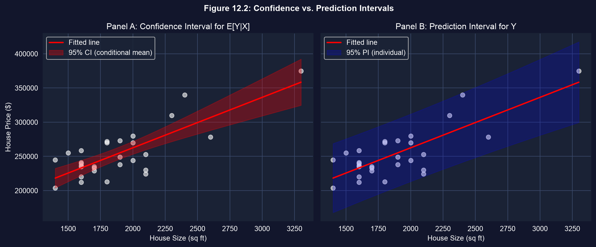
The individual carries an extra, irreducible term $u^*$ — the “$1+$” under the square root that never shrinks, even with infinite data.

Predict a price — and both kinds of interval

from scipy import stats                      # t-distribution for interval widths

fit = pf.feols("price ~ size", data=data)    # simple regression on size

x = data["size"].values; xbar = x.mean()     # ingredients for the SE formulas
Sxx = ((x - xbar)**2).sum(); n = len(data)

s_e = np.sqrt((fit._u_hat**2).sum() / (n - 2))   # RMSE — the irreducible noise floor s_e
pred = fit.predict(newdata=pd.DataFrame({"size": [2000]}))[0]  # point prediction at 2000 sq ft

t = stats.t.ppf(0.975, n - 2)                # 95% critical value, df = n − 2
se_cm = s_e * np.sqrt(1/n + (2000 - xbar)**2 / Sxx)        # conditional-MEAN SE
se_pi = s_e * np.sqrt(1 + 1/n + (2000 - xbar)**2 / Sxx)    # INDIVIDUAL SE (note the leading 1)

print(pred, t*se_cm, t*se_pi)                # point, CI half-width, PI half-width

↗ Try it in Colab

The prediction interval is ~5× wider — and stays that way

Panel A: the narrow 95% CI for the average 2{,}000-sq-ft price. Panel B: the much wider 95% PI for one house. The funnel widens away from the data’s center.

For a 2{,}000-sq-ft house: point ≈ $263k · CI ≈ [$253k, $272k] · PI ≈ [$213k, $312k]. More data narrows the CI, barely touches the PI.

A biased sample can break the line itself

Selection on $X$ (e.g. oversample large houses) — OLS stays unbiased if $X$ is in the model; you only lose precision.
Selection on $Y$ (e.g. survey drops top earners) — OLS is biased for the population; needs sample weights, a Heckman correction, or a selection model.

No robust SE repairs a bad sample. Always ask whether the sample represents the population you care about.

Best estimators, and the limits of a test

Act III · The resolution

OLS is “best” — until its assumptions fail

Under the classical assumptions, OLS is BLUE (Best Linear Unbiased Estimator) by the Gauss–Markov theorem. When homoskedasticity or independence fails, OLS stays unbiased but is no longer most efficient — feasible GLS (FGLS) can be tighter.

In practice, most applied work keeps OLS with robust SEs: the efficiency loss is small, and a misspecified GLS weighting model can do more harm than good.

Default to OLS + robust SEs. Reach for FGLS only when you trust the error-variance model.

The bootstrap: let the data draw its own distribution

Instead of trusting a normal approximation, resample the data with replacement ~1,000 times, re-estimate each time, and read the 2.5th and 97.5th percentiles of the resulting coefficients as a 95% CI.

The bootstrap assumes no normality and works for awkward statistics — ideal for small samples like these $n = 29$ houses.

Every test trades off two ways to be wrong

Decision	$H_0$ true	$H_0$ false
Reject $H_0$	Type I error ($\alpha$)	Correct — power
Don’t reject	Correct	Type II error ($\beta$)

Tightening $\alpha$ cuts false positives but raises $\beta$ — fewer real effects detected. Power $= 1-\beta$ is the probability of catching a true effect.

With only $n=29$, the bedrooms test failed to reject ($p=0.773$) — likely a Type II miss, not proof of “no effect”.

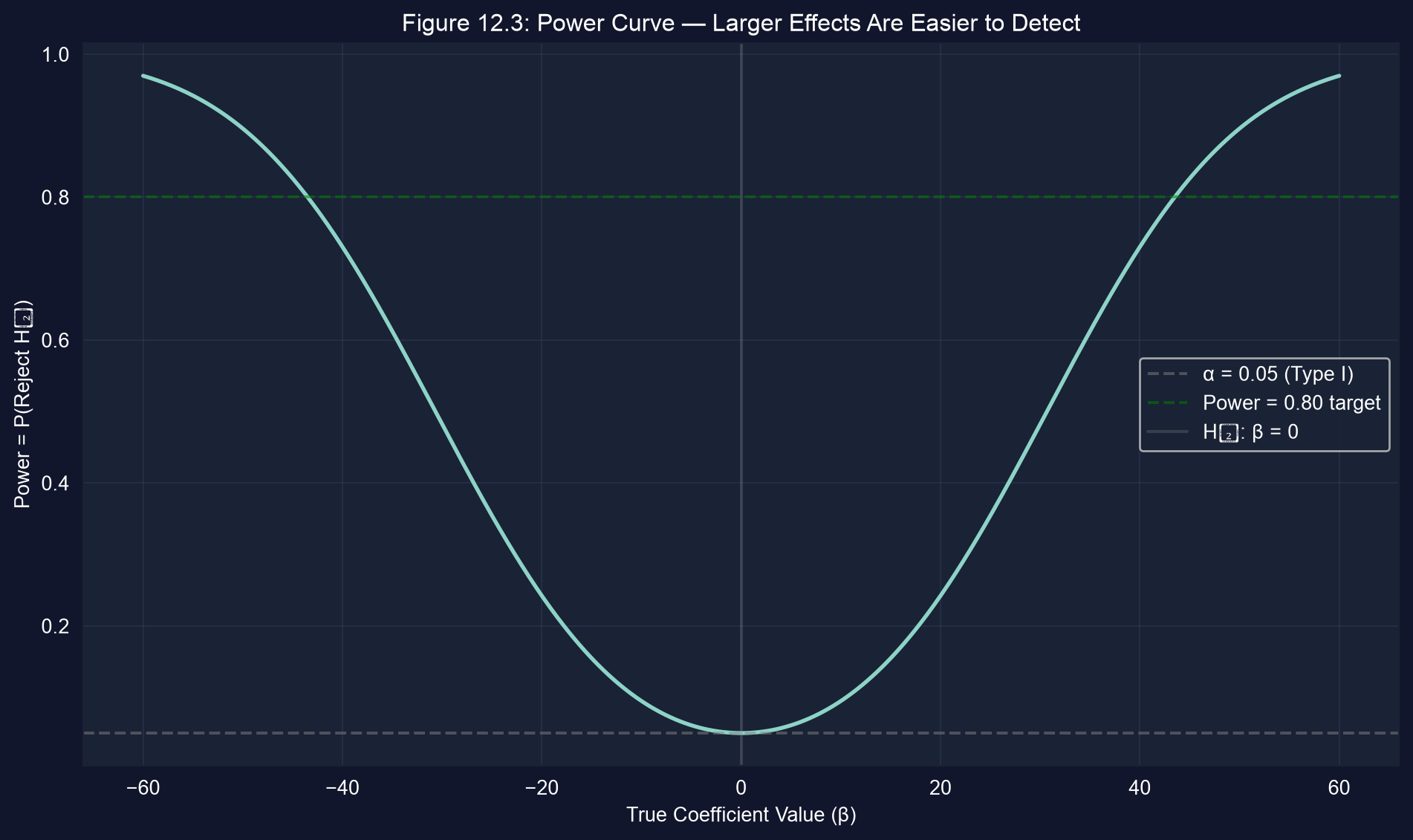
Power rises with effect size — and with the sample

Power curve at $n=30$, SE $=15$, $\alpha=0.05$. Power equals $\alpha$ at $\beta=0$ and climbs toward 1 as the true effect grows.

from scipy import stats; import numpy as np  # distributions + numerics

alpha, se, n = 0.05, 15, 30                  # significance, hypothetical SE, sample size
tcrit = stats.t.ppf(1 - alpha/2, df=n - 1)   # two-sided critical value
betas = np.linspace(-60, 60, 500)            # grid of true effect sizes to evaluate

ncp = betas / se                             # non-centrality: effect in SE units
power = 1 - (stats.t.cdf(tcrit - ncp, n - 1) # P(reject | true β) under the alternative
             - stats.t.cdf(-tcrit - ncp, n - 1))

# here power reaches the 0.80 target only around |β| ≈ 43.5 — small effects need a bigger n
print(betas[(betas > 0) & (power >= 0.80)].min())

↗ Try it in Colab

What to carry forward

OLS coefficients survive heteroskedasticity, clustering, and autocorrelation — the SEs need repair: HC1 / cluster / HAC.
The fix is cheap: one vcov= keyword, or an intercept-only HAC fit for a time-series mean.
Predicting an average is precise; predicting an individual is not — the “$1+$” floor is $\approx s_e$ forever.
Selection on $Y$ biases; selection on $X$ only costs precision — robust SEs can’t rescue a bad sample.
OLS + robust SEs is the safe default; the bootstrap sidesteps normality; power decides what a null result means.

Trust the line, repair the uncertainty — and respect what a sample can’t tell you.

Decision	\(H_0\) true	\(H_0\) false
Reject \(H_0\)	Type I error (\(\alpha\))	Correct — power
Don’t reject	Correct	Type II error (\(\beta\))

When the standard assumptions break

OLS gives the right line — but can lie about how sure we are

Where we’re going

Six ideas anchor this chapter

Repairing the standard errors

Three violations, three fixes — coefficients never change

Robust SEs are one keyword: vcov="HC1"

For these houses, robust SEs tell the same story

Time series carry an echo — the correlogram shows it

HAC (Newey–West) SEs account for that echo

Prediction splits in two: the average vs. the individual

Predict a price — and both kinds of interval

The prediction interval is ~5× wider — and stays that way

A biased sample can break the line itself

Best estimators, and the limits of a test

OLS is “best” — until its assumptions fail

The bootstrap: let the data draw its own distribution

Every test trades off two ways to be wrong

Power rises with effect size — and with the sample

What to carry forward

Trust the line, repair the uncertainty — and respect what a sample can’t tell you.

Robust SEs are one keyword: `vcov="HC1"`