Nine questions, one toolkit

Act I · The tension

Welcome to the chapter that pulls the whole book together. Every case study uses the same estimator (OLS, and in 13.8 its IV cousin) on a different real dataset. What changes from case to case is the question, the data structure, the standard errors, and — above all — the source of variation that lets us interpret a slope.

Regression describes — but can it explain why?

By now we can fit a line, add controls, and read a slope. But a slope is an association: schools with better-educated parents score higher; countries with stronger property rights are richer. Does the regressor cause the outcome?

This chapter works through nine case studies on real data. The first four push observational regression as far as it goes. The last four bring in a research design (an RCT, difference-in-differences, a regression discontinuity, or an instrumental variable) that turns a slope into a causal claim.

The question running through every case is the same: where does the variation in the regressor come from?

Frame the deck as a climb: describe → specify → diagnose bias → design for causation. Each case is self-contained, with its own data, code, output and interpretation, so you can teach any case on its own. Use the agenda on the next slide to jump.

Nine case files — click any case to jump to it

Case	Question	Method	Headline result
13.1	What drives school test scores?	Multiple regression	+73.9 API points per year of parent ed.
13.2	Constant returns to scale?	Cobb–Douglas, HAC SEs	elasticities sum to 1.04 (p = 0.636)
13.3	Why did the Phillips curve break?	Omitted variables bias	+0.265 = −0.128 + 1.146 × 0.343
13.4	What determines fuel economy?	Log-log, clustered SEs	weight elasticity −0.56
13.5	Does cost-sharing cut spending?	RCT	95% plan: −$1,108 vs free care
13.6	Did free care help child nutrition?	Diff-in-differences	+0.52 weight-for-age z-units
13.7	Does holding a seat help a party?	Regression discontinuity	+4.8 percentage points
13.8	Do institutions cause prosperity?	Instrumental variables	IV 0.94 vs OLS 0.52
13.9	How does raw data become final data?	Read, merge, clean	—

Cases 13.1–13.4 are observational; 13.5–13.8 are designs for causation; 13.9 is the workflow underneath them all.

The case numbers are links: click one to jump straight to that case’s divider. Press M for the menu (every slide title is listed) or O for the overview grid. Every case follows the same arc: question → data → method → code → output → interpretation → caveats.

The climb: from description to causation

• Describe (13.1, 13.4): conditional associations, with controls and honest SEs
• Impose structure (13.2): a theory-based functional form makes the coefficients interpretable as elasticities and gives a testable restriction
• Diagnose bias (13.3): the omitted-variables formula tells us how much a missing regressor distorts a slope
• Design for causation (13.5–13.8): an RCT, DiD, RD or IV builds a credible counterfactual

Controls can only close the confounders we measure. A design closes the ones we don’t.

The ladder idea: each rung adds an assumption that is easier to defend. Description makes no causal claim. Structure adds theory. The OVB formula tells us the direction and size of bias. Designs replace “I controlled for everything” (unverifiable) with a specific, defensible identifying assumption: random assignment, parallel trends, continuity at a cutoff, or an exclusion restriction.

One estimator, three ways to be honest about uncertainty

SE type	pyfixest syntax	Use when errors are…	Cases
Heteroskedasticity-robust	vcov="HC1"	independent, unequal variance (cross-sections)	13.1, 13.7, 13.8
HAC (Newey–West)	vcov="NW" + time_id, lag	autocorrelated over time (time series)	13.2, 13.3
Cluster-robust	vcov={"CRV1": "group"}	correlated within groups	13.4 (maker), 13.5 (family), 13.6 (community)

The coefficient is identical under all three. Only the standard errors, and therefore the \(t\)-statistics, \(p\)-values and confidence intervals, change.

Match the standard error to how the data were generated. In 13.4, clustering makes the SEs 6–9× larger than HC1.

The chapter uses one estimation function, pf.feols, throughout. The vcov argument changes only the inference. HC1 handles heteroskedasticity across independent observations. Newey–West (HAC) also allows correlation between nearby time periods — the chapter uses 3 lags for the 24-year Cobb–Douglas series and 5 lags for the 45-year post-1970 Phillips series. CRV1 allows arbitrary correlation inside each cluster (manufacturer, family, community). We will see in 13.4 that this choice is not cosmetic.

Five ideas anchor this chapter

• Production function: inputs \(\to\) output. Cobb–Douglas \(Q = AK^{\beta_2}L^{\beta_3}\) is linear in logs
• Constant returns to scale: doubling every input doubles output, i.e. \(\beta_2 + \beta_3 = 1\)
• Selection bias: treated and untreated units differ before treatment; random assignment removes the difference
• Parallel trends: the DiD assumption that, without treatment, both groups would have moved together
• Counterfactual: the unobserved “what would have happened”; every design imputes it differently

A credible causal estimate is not a better regression. It is a better source of variation.

These are the chapter’s Key Concepts. Production function and CRS anchor 13.2; selection bias anchors 13.5; parallel trends anchors 13.6; the counterfactual idea ties 13.5–13.8 together.

Act II-a · Observational regression, pushed to its limits

Cases 13.1–13.4 · describe, structure, diagnose

Four cases with observational data. None claims causality in the strict sense; each teaches a tool: controls and multicollinearity (13.1), logs and testing a restriction (13.2), the OVB formula (13.3), and clustering (13.4).

Case 13.1 · What drives school performance?

Multiple regression · cross-section · HC1 standard errors

Case 13.1: the California Academic Performance Index. Tools: bivariate vs multiple regression, correlation matrix, multicollinearity, reading partial effects.

The question: family background or school resources?

Data. 807 California high schools, 1999 (AED_API99.DTA). The Academic Performance Index (API) runs from 200 to 1000; the state target is 800.

Variable	Meaning
api99	Academic Performance Index, 1999 (outcome)
edparent	average parent education, in years
meals	% of students in the free / reduced-price lunch program (poverty proxy)
englearn	% English learners
yearround	1 if the school runs a multi-track year-round calendar
credteach, emerteach	% of teachers with full / emergency credentials

Every regressor is the result of choices by families, districts or teachers, so expect associations, not causal effects.

Economic question: what determines school performance, resources (teachers) or demographics (parents’ education, poverty, language)? Nothing here is randomly assigned. Families choose where to live, teachers sort across schools, districts pick calendars. Keep that in mind for the interpretation.

Most schools fall well short of the 800 target

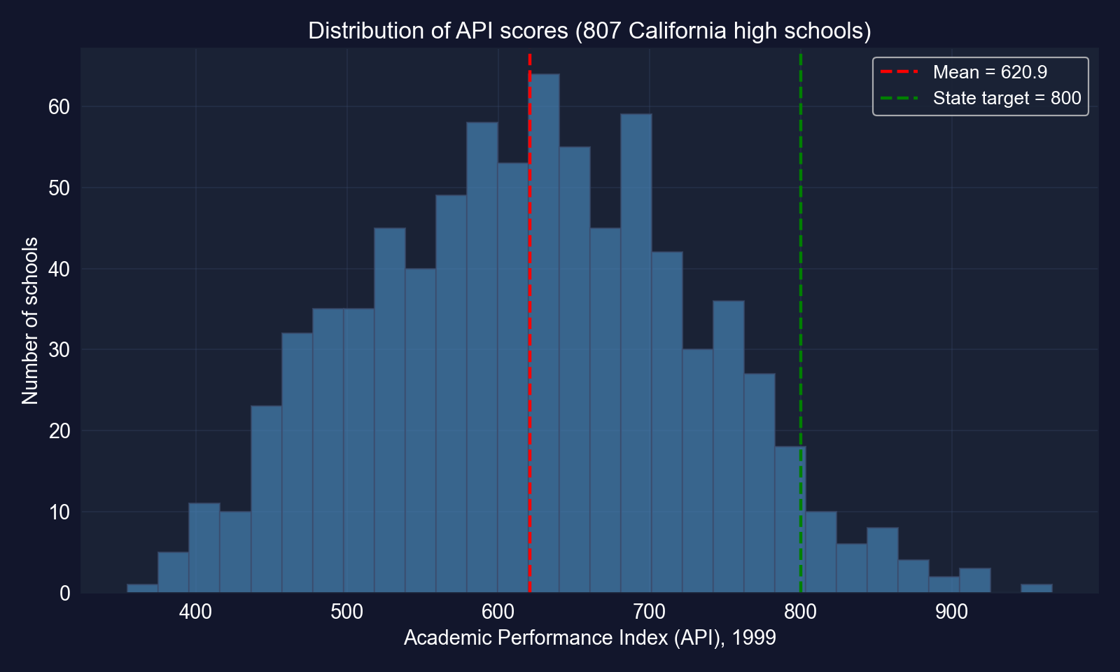
Distribution of 1999 API scores across 807 high schools. Red: mean (620.9); green: the state target of 800.

The mean school scores about 621, and only 4.8% of schools reach 800, so the outcome varies enough to explain.

Roughly symmetric (skewness ≈ 0.12, very slightly right-skewed). Scores range from below 400 to above 900. Mean 620.9. Only 4.8% of schools have API ≥ 800 (computed from the same data). Lots of variation to explain.

Code: load the data and fit the bivariate regression

!pip install -q pyfixest                    # pyfixest is not preinstalled in Colab
import pandas as pd                         # tabular data
import pyfixest as pf                       # OLS / IV with R-style formulas
# 807 California high schools, 1999
url = "https://raw.githubusercontent.com/quarcs-lab/data-open/master/AED/AED_API99.DTA"
data_api = pd.read_stata(url)               # read the Stata file into a DataFrame
vars_api = ["api99", "edparent", "meals", "englearn", "yearround", "credteach", "emerteach"]
data_api[vars_api].describe()               # summary statistics for the 7 variables
fit_api_biv = pf.feols("api99 ~ edparent", data=data_api, vcov="HC1")  # bivariate OLS
fit_api_biv.summary()                       # intercept, slope, robust SE, R²

↗ Try it in Colab

Self-contained: paste into an empty Colab cell. vcov=“HC1” requests heteroskedasticity-robust standard errors, appropriate for a cross-section of independent schools.

Output: one predictor explains 83.5% of the variation

	Coef.	SE	\(t\)
Intercept	−400.314	15.993	−25.03
edparent	79.529	1.219	65.25

N = 807 · HC1 SEs · \(R^2 = 0.835\) · 95% CI for slope: [77.14, 81.92]

Each additional year of average parent education is associated with 79.5 more API points.

API vs parent education, with the OLS line.

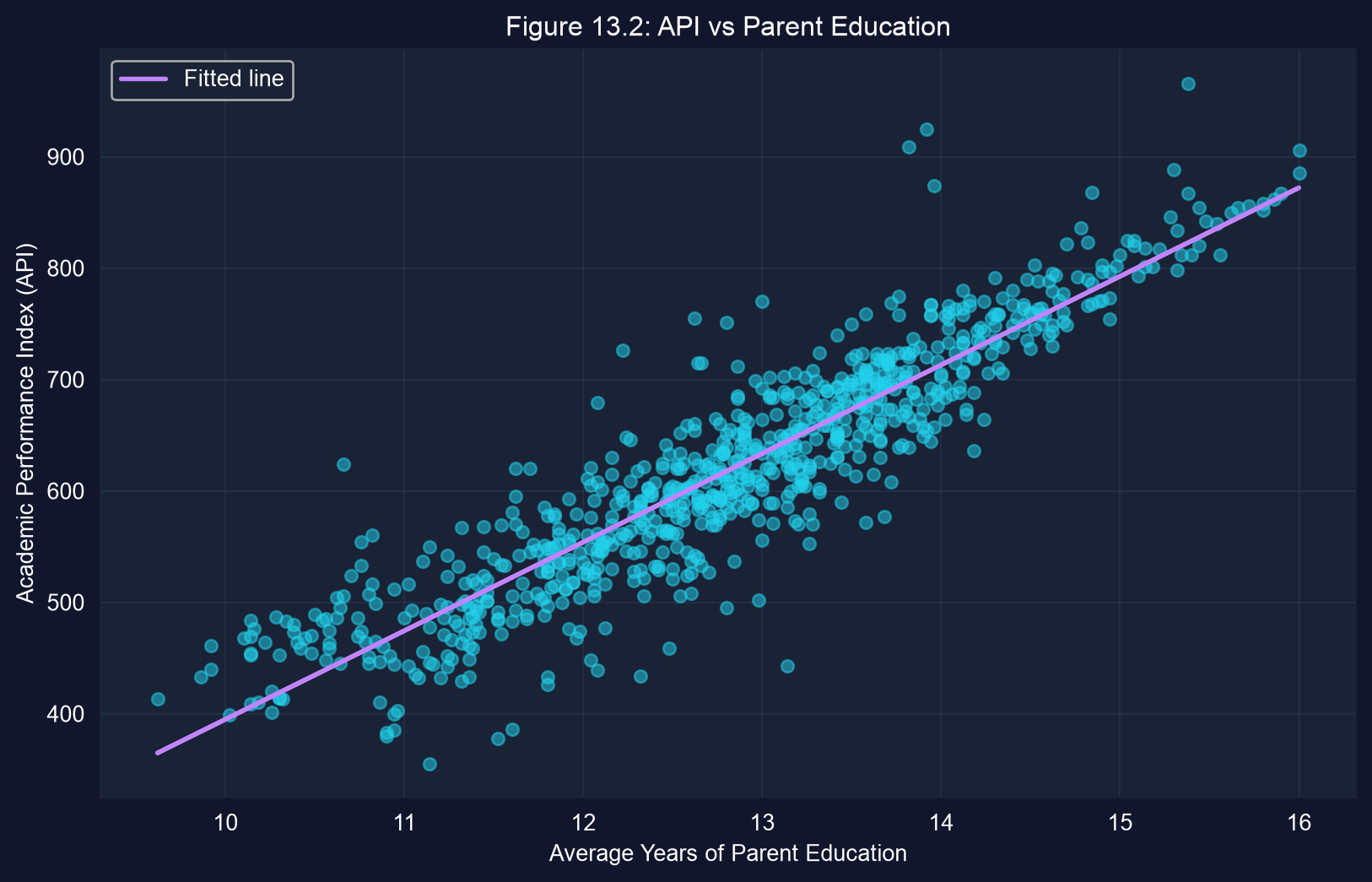
A huge, precise slope, but edparent also stands in for income, language and neighbourhood. Next, we add controls.

Estimated equation: API = −400.3 + 79.5 × edparent. R² = 0.835, which is unusually high for a cross-section. The intercept is an extrapolation (zero years of education is outside the data, which run from 9.6 to 16 years) and has no meaning on its own. The bivariate slope bundles everything correlated with parent education.

Code: are the regressors themselves correlated?

# continues from the previous block (data_api, vars_api already defined)
import seaborn as sns                       # statistical plotting (heatmap)
import matplotlib.pyplot as plt             # figure handling
corr_matrix = data_api[vars_api].corr()     # pairwise Pearson correlations
print(corr_matrix.round(2))                 # numeric matrix, 2 decimals
sns.heatmap(corr_matrix, annot=True, fmt=".2f", cmap="coolwarm", center=0)  # coloured matrix
plt.show()                                  # display the heatmap

↗ Try it in Colab

Before adding controls, check how strongly they move together. That decides how precisely their separate effects can be estimated.

A correlation matrix is the quickest multicollinearity diagnostic. Strongly correlated regressors carry overlapping information, so OLS has little independent variation left to tell their effects apart.

Output: the regressors are strongly correlated

Correlation matrix of API and its six candidate determinants.

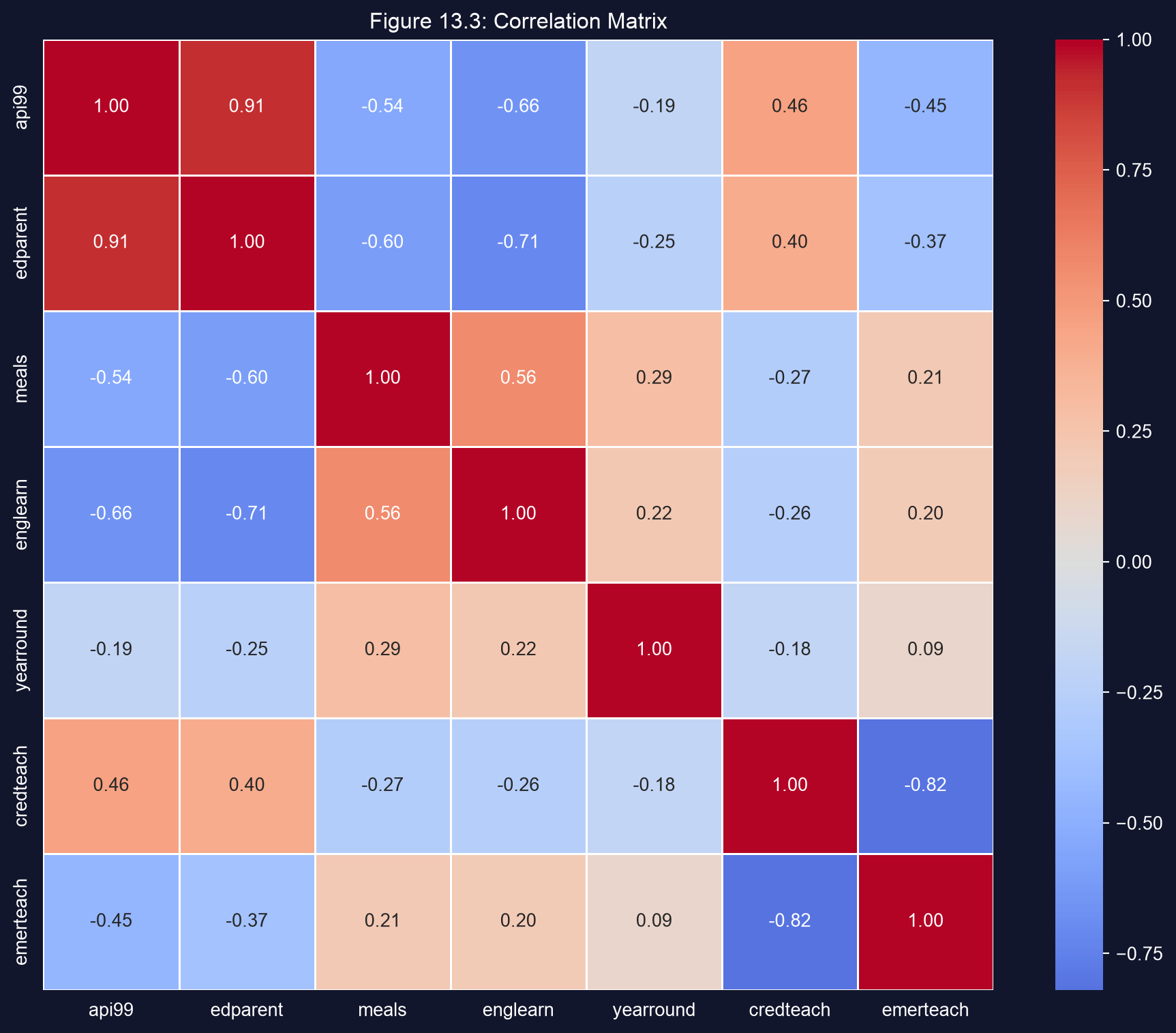
Pair	\(r\)
api99–edparent	0.91
api99–englearn	−0.66
api99–meals	−0.54
edparent–englearn	−0.71
edparent–meals	−0.60
credteach–emerteach	−0.82

Parent education, poverty and English learners largely describe the same schools, so their separate effects will be hard to pull apart.

Strong negative correlations of API with meals (−0.54) and englearn (−0.66); strong positive with edparent (0.91). Among regressors: edparent–englearn −0.71, edparent–meals −0.60, and the two teacher-credential variables −0.82, which are nearly mirror images. Expect inflated standard errors on whichever of these overlapping variables carries less unique information.

Code: the multiple regression

# continues from the previous block
fit_api_mult = pf.feols("api99 ~ edparent + meals + englearn + yearround + credteach + emerteach",
                        data=data_api, vcov="HC1")   # six regressors, robust SEs
fit_api_mult.summary()                               # full coefficient table
coef_df = pd.DataFrame({                             # compact table of results
    "Coefficient": fit_api_mult.coef(),              # point estimates
    "Std Error": fit_api_mult.se(),                  # HC1 standard errors
    "t-stat": fit_api_mult.tstat(),                  # coefficient / SE
    "p-value": fit_api_mult.pvalue()                 # two-sided p-values
}).round(3)
print(coef_df)

↗ Try it in Colab

Same data, six regressors. Each coefficient is now a partial effect: the association with API holding the other five regressors fixed.

Output: parent education survives every control

Variable	Coef.	SE	\(t\)	\(p\)	95% CI
Intercept	−345.328	44.027	−7.84	< 0.001	[−431.75, −258.91]
edparent	73.942	1.835	40.29	< 0.001	[70.34, 77.54]
meals	0.079	0.092	0.86	0.390	[−0.10, 0.26]
englearn	−0.358	0.177	−2.02	0.044	[−0.71, −0.01]
yearround	25.956	10.752	2.41	0.016	[4.85, 47.06]
credteach	0.387	0.349	1.11	0.268	[−0.30, 1.07]
emerteach	−1.470	0.358	−4.11	< 0.001	[−2.17, −0.77]

N = 807 · HC1 SEs · \(R^2 = 0.853\) (vs 0.835 with edparent alone)

With five controls, the parent-education slope falls only from 79.5 to 73.9, and the controls add just 1.8 points of \(R^2\).

Key Concept 13.1: the parent-education coefficient stays around 74 points even after controlling for meals, English learners, year-round calendars and teacher credentials. The jump in R² is small because edparent already captures most of what the other variables measure.

Reading the coefficients (1): what “holding constant” means

• edparent 73.9: comparing schools with the same poverty, language, calendar and credential mix, one more year of parent education goes with 73.9 more API points
• meals 0.08 (\(p = 0.39\)): on its own, poverty correlates \(-0.54\) with API, but once parent education is held fixed it adds no separate predictive information
• That does not mean poverty is irrelevant: it overlaps heavily with edparent (\(r = -0.60\)), so the data cannot separate the two

A partial effect answers “compared with otherwise-similar schools…”, and the answer depends on which variables we hold fixed.

Interpret each coefficient as a comparison between schools that are alike on every other regressor. An insignificant coefficient on a highly collinear variable (meals) says “no detectable separate association given the others”, not “zero effect”.

Reading the coefficients (2): collinearity and sign changes

• emerteach −1.47 per percentage point: more emergency-credentialed teachers, lower scores (\(p < 0.001\))
• Its mirror image credteach is insignificant (\(p = 0.27\)): the two are correlated \(-0.82\), so they compete for the same variation
• yearround +26.0 (\(p = 0.016\)): year-round schools score 26 points higher conditional on the rest, although the simple correlation is negative (\(-0.19\))

Collinear regressors share credit unpredictably, and conditioning can flip a sign, which previews the omitted-variables lesson of 13.3.

credteach and emerteach nearly mirror each other (fully credentialed vs emergency credentials), so whichever enters with more unique variation absorbs the effect. The yearround sign change is a small preview of 13.3: what you condition on changes the slope.

Why these are associations, not causal effects

What the regression holds fixed

• the six measured characteristics
• nothing else

What it cannot hold fixed

• family income, home resources, private tutoring
• which families choose which districts
• how teachers sort toward easier schools

edparent is a proxy for a whole bundle of advantages, so 73.9 is a conditional association, not “the effect of sending parents back to school”.

Standard caveat for observational regression: omitted variables correlated with both edparent and API (income, wealth, neighbourhood) load onto the edparent coefficient. Selection of families into districts and of teachers into schools also breaks any causal reading. The chapter notes California’s “similar schools” index, which uses exactly this kind of regression to benchmark schools against comparable peers: a descriptive use for which conditional associations are fine.

Case 13.2 · Does doubling inputs double output?

Cobb–Douglas production function · log-log model · HAC standard errors

Case 13.2: Douglas’s U.S. manufacturing data, 1899–1922. Tools: log transformation, elasticities, a test of a linear restriction, retransformation of log predictions, HAC standard errors for time series.

The question: returns to scale in U.S. manufacturing

The Cobb–Douglas production function maps capital \(K\) and labor \(L\) into output \(Q\):

\[Q = A\,K^{\beta_2}\,L^{\beta_3}\]

If \(\beta_2 + \beta_3\) is…	Returns to scale	Doubling both inputs…
\(= 1\)	constant	doubles output
\(> 1\)	increasing	more than doubles output
\(< 1\)	decreasing	less than doubles output

Returns to scale come down to a single number, \(\beta_2 + \beta_3\), which we can estimate and test.

A is total factor productivity (the technology level). β₂ and β₃ are the output elasticities of capital and labor. Scaling both inputs by λ multiplies output by λ^(β₂+β₃), which is why the sum decides returns to scale. Competitive-market theory often predicts constant returns.

Taking logs turns a multiplicative model into a linear regression

\[\ln Q = \underbrace{\ln A}_{\beta_1} + \beta_2 \ln K + \beta_3 \ln L + u\]

The model is now linear in its parameters, so OLS applies. Each slope is an elasticity: \(\beta_2 = \partial \ln Q / \partial \ln K\), the percentage change in output per 1% change in capital, holding labor fixed.

Logs do two jobs here: they make the model estimable by OLS, and they make the coefficients unit-free elasticities.

Key Concept 13.2. Because both sides are in logs, a coefficient measures a proportional response. Strictly, “a 1% change in K changes Q by β₂%” is a marginal (calculus) statement; for finite changes it is an approximation that is excellent for small changes.

The data: 24 years of output, capital and labor (1899 = 100)

Index in 1922	Value	Growth since 1899
Output \(Q\)	240	2.4×
Capital \(K\)	431	4.3×
Labor \(L\)	161	1.6×

Why HAC standard errors?

• Time series: booms, recessions and technology shocks persist, so errors are autocorrelated
• Volatility differs across periods (e.g. World War I), so errors are heteroskedastic
• Newey–West (HAC) SEs allow for both; the chapter uses 3 lags

Capital grew much faster than output or labor. How the regression splits output growth between the two inputs is the elasticity question.

Douglas (1976) data; all series are indices with 1899 = 100. Default OLS SEs assume uncorrelated, homoskedastic errors, which is wrong here. HC1 fixes heteroskedasticity but ignores autocorrelation. HAC (heteroskedasticity- and autocorrelation-consistent) SEs fix both. With only 24 observations, even HAC SEs are themselves imprecise.

Code: log-transform and estimate with Newey–West SEs

!pip install -q pyfixest                    # pyfixest is not preinstalled in Colab
import numpy as np                          # np.log for the transform
import pandas as pd                         # tabular data
import pyfixest as pf                       # OLS with R-style formulas
url = "https://raw.githubusercontent.com/quarcs-lab/data-open/master/AED/AED_COBBDOUGLAS.DTA"
data_cobb = pd.read_stata(url)              # 24 years of U.S. manufacturing, 1899–1922
data_cobb["lnq"] = np.log(data_cobb["q"])   # log output
data_cobb["lnk"] = np.log(data_cobb["k"])   # log capital
data_cobb["lnl"] = np.log(data_cobb["l"])   # log labor
data_cobb["_time"] = range(len(data_cobb))  # time index required by Newey–West
fit_cobb = pf.feols("lnq ~ lnk + lnl", data=data_cobb,
                    vcov="NW", vcov_kwargs={"time_id": "_time", "lag": 3})  # HAC SEs, 3 lags
fit_cobb.summary()                          # elasticities, HAC SEs, R²

↗ Try it in Colab

Self-contained. Note vcov=“NW” with a time index and lag = 3. This is the chapter’s specification; plain OLS SEs would ignore the autocorrelation in this time series.

Output: labor’s elasticity is about 3.5× capital’s

Variable	Coef.	HAC SE	\(t\)	\(p\)	95% CI
Intercept	−0.177	0.398	−0.45	0.660	[−1.000, 0.646]
lnk (capital)	0.233	0.063	3.72	0.001	[0.103, 0.363]
lnl (labor)	0.807	0.135	6.00	< 0.001	[0.529, 1.086]

N = 24 · Newey–West SEs, 3 lags · \(R^2 = 0.957\)

• Holding labor fixed, a 1% increase in capital is associated with ≈ 0.23% more output
• Holding capital fixed, a 1% increase in labor is associated with ≈ 0.81% more output

Early-1900s manufacturing was labor-driven: the labor elasticity (0.81) is about 3.5 times the capital elasticity (0.23).

Estimated equation: ln Q = −0.177 + 0.233 ln K + 0.807 ln L. The “≈” matters: elasticities describe small proportional changes; for a large change, compute (1+Δ)^β − 1 instead. Labor/capital ratio of elasticities: 0.807 / 0.233 ≈ 3.46. The very high R² partly reflects that all three series trend upward together (see the caveats slide).

Code: test constant returns with the HAC covariance matrix

# continues from the previous block
from scipy import stats                     # F distribution for the p-value
R = np.array([0.0, 1.0, 1.0])               # restriction vector: picks out β_K + β_L
b_hat = fit_cobb.coef().values              # coefficients [Intercept, lnk, lnl]
V_hac = fit_cobb._vcov                      # Newey–West (HAC) covariance matrix
df_resid = fit_cobb._N - len(b_hat)         # residual degrees of freedom: 24 − 3 = 21
f_stat = (R @ b_hat - 1.0)**2 / (R @ V_hac @ R)   # Wald statistic for H0: β_K + β_L = 1
p_value = 1 - stats.f.cdf(f_stat, 1, df_resid)    # p-value from F(1, 21)
print(R @ b_hat, f_stat, p_value)           # estimated sum, F, p

↗ Try it in Colab

The test reuses the HAC covariance matrix, so the inference matches the HAC standard errors on the previous slide.

Key Concept 13.3: a test of one linear restriction on two coefficients. A classical restricted-vs-unrestricted F test would assume iid errors, which we have already argued against; the Wald form with V_HAC is robust. R·b̂ is the estimated sum; R·V·Rᵀ is its variance.

Output: the data are consistent with constant returns to scale

Quantity	Value
\(\hat\beta_K + \hat\beta_L\)	1.040
HAC SE of the sum	0.084
\(F(1, 21)\)	0.23
\(p\)-value	0.636
95% CI for the sum	[0.87, 1.21]

• \(H_0: \beta_K + \beta_L = 1\) is not rejected at any conventional level
• But the 95% interval spans 0.87 to 1.21: mild decreasing or increasing returns also fit the data
• “Fail to reject” is not “prove”. With 24 years, the test has limited power

The estimate (1.04) is close to 1 and statistically indistinguishable from it, which supports constant returns without proving them.

The chapter reports F = 0.23 and p = 0.636. The 95% CI uses the same HAC SE (0.084) and t(21) = 2.08: 1.040 ± 2.08 × 0.084 ≈ [0.87, 1.21]. This interval is derived arithmetic from the chapter’s output, not a new estimate. Present the result honestly: the evidence is consistent with CRS, and also consistent with modest departures from it.

The fitted model tracks output across 24 years

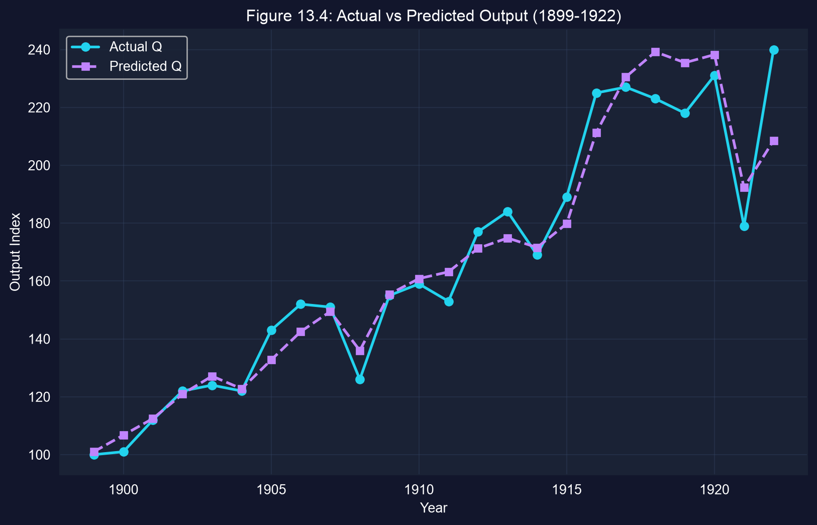
Actual vs predicted output, 1899–1922. Predictions are \(e^{\widehat{\ln Q}}\) multiplied by the retransformation factor \(e^{\hat\sigma^2/2}\).

To predict levels from a log model, exponentiate and rescale by \(e^{\hat\sigma^2/2}\); here \(\hat\sigma = 0.058\), so the correction is tiny (×1.0017).

Code (in the chapter): se = sqrt(Σû² / (N − k)); q_pred = exp(se²/2) · exp(fitted ln Q). Because E[e^u] = e^(σ²/2) > 1 for normal errors, simply exponentiating fitted logs under-predicts the mean level. Here σ̂ = 0.058, so the factor is 1.0017. The predicted series follows actual output closely, with the largest misses in the 1920–22 swings.

Caveats: why 24 trending observations call for humility

• Trending series: \(Q\), \(K\) and \(L\) all rise over time, so part of the \(R^2 = 0.957\) is a shared trend, not a production relationship (the spurious-regression worry)
• Technology held constant: \(A\) is a single constant; omitted technical progress that grew with capital would load onto \(\hat\beta_K\)
• Small sample: 24 points, and HAC SEs are themselves noisy with so few years
• Aggregation: one “representative” manufacturing sector stands in for many industries

The CRS test is informative, but treat the separate elasticities as fragile.

These are standard caveats for an aggregate time-series production function, not results the chapter computes. The spurious-regression problem (regressing one trending series on another) is covered in time-series chapters. A natural extension would add a time trend to proxy technical change; this deck does not estimate it.

Case 13.3 · Why did the Phillips curve break?

Omitted variables bias · time series · HAC standard errors

Case 13.3: the most important diagnostic case in the chapter. The same two variables give opposite slopes in two periods; the omitted-variables-bias formula explains exactly why.

The question: is there a stable unemployment–inflation trade-off?

• Phillips (1958): lower unemployment went with higher wage inflation, so policymakers saw a menu: choose a point on the curve
• 1970s stagflation: high unemployment and high inflation together, and the menu fell apart
• Friedman–Phelps: the curve shifts with expected inflation; leave expectations out and the curve is misspecified

\[\text{Inflation}_t = \beta_1 + \beta_2\,\text{Urate}_t + \beta_3\,\text{ExpInflation}_t + u_t\]

If expected inflation belongs in the model, omitting it is not harmless. It can distort, even reverse, the unemployment slope.

Data: AED_PHILLIPS.DTA, U.S. 1949–2014 (66 years). inflgdp = annual inflation from the GDP deflator (%); urate = civilian unemployment rate (%); inflgdp1yr = one-year-ahead expected inflation from the Survey of Professional Forecasters. In this dataset the expectations series is available only from 1970 onward, so the augmented model can only be run post-1970.

Code: the pre-1970 Phillips curve

!pip install -q pyfixest                    # pyfixest is not preinstalled in Colab
import pandas as pd                         # tabular data
import pyfixest as pf                       # OLS with R-style formulas
url = "https://raw.githubusercontent.com/quarcs-lab/data-open/master/AED/AED_PHILLIPS.DTA"
data_phillips = pd.read_stata(url)          # U.S. annual data, 1949–2014
data_pre1970 = data_phillips[data_phillips["year"] < 1970].copy()   # 1949–1969
data_pre1970["_time"] = range(len(data_pre1970))                    # time index for HAC
fit_pre = pf.feols("inflgdp ~ urate", data=data_pre1970,
                   vcov="NW", vcov_kwargs={"time_id": "_time", "lag": 3})  # HAC, 3 lags
fit_pre.summary()                           # slope on unemployment

↗ Try it in Colab

Self-contained. 21 annual observations, 1949–1969, Newey–West SEs with 3 lags.

Output: before 1970, the trade-off is there

	Coef.	HAC SE	\(p\)
Intercept	7.106	1.581	< 0.001
urate	−1.030	0.325	0.005

N = 21 (1949–1969) · NW, 3 lags · \(R^2 = 0.454\)

One percentage point more unemployment is associated with about 1.03 percentage points less inflation.

1949–1969: inflation vs unemployment, with the OLS line.

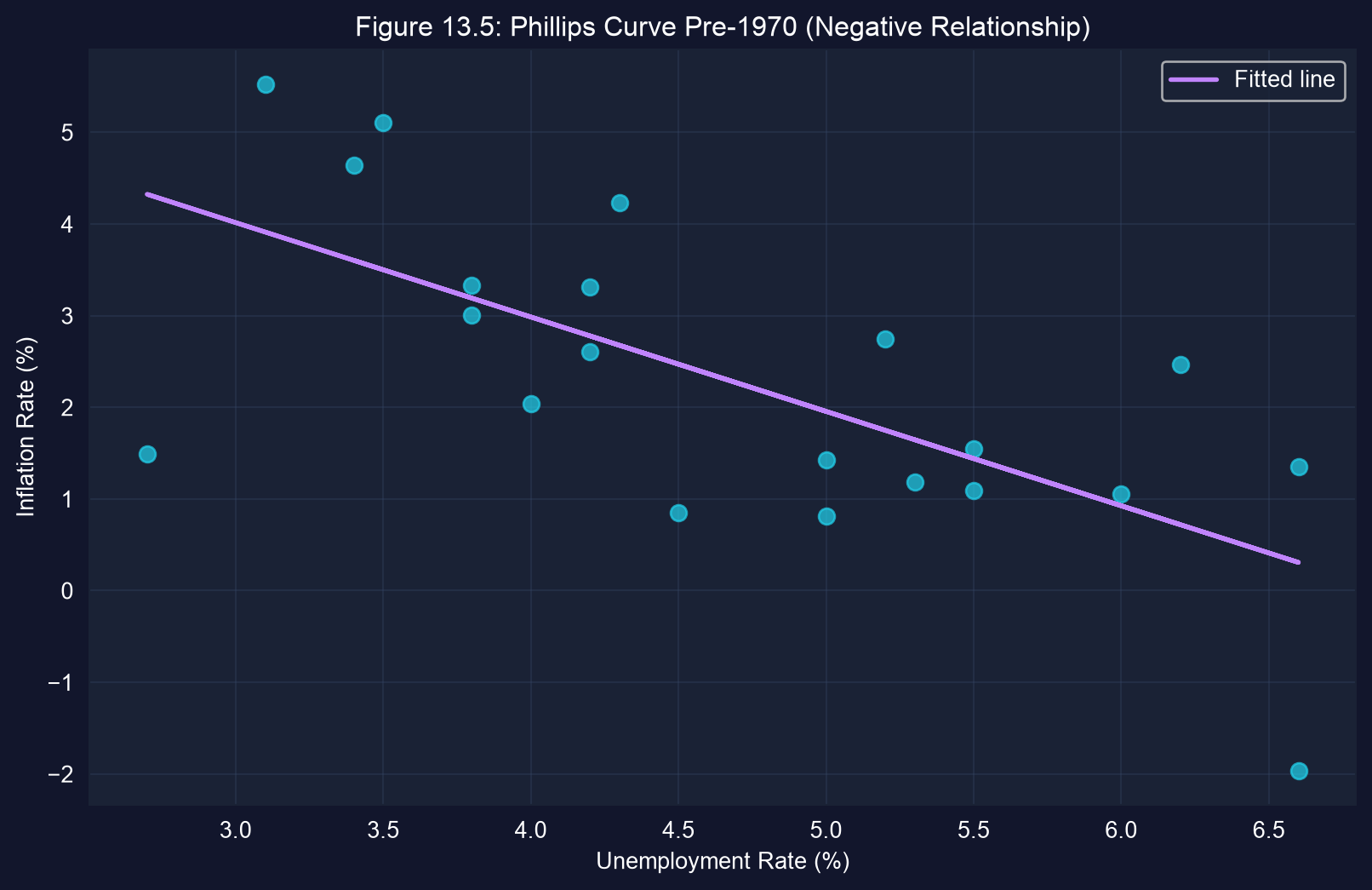
The classic downward-sloping Phillips curve: negative and statistically significant (\(p = 0.005\)).

Both variables are measured in percent, so the slope is in percentage points per percentage point, not “1%” in the proportional sense. The chapter’s explanation for why the simple curve worked then: expected inflation was low and stable in the 1950s–60s, so omitting it did little damage. (This dataset cannot check that directly, because the SPF expectations series starts in 1970.)

Code: the same regression after 1970

# continues from the previous block
data_post1970 = data_phillips[data_phillips["year"] >= 1970].copy()  # 1970–2014
data_post1970["_time"] = range(len(data_post1970))                   # time index for HAC
fit_post = pf.feols("inflgdp ~ urate", data=data_post1970,
                    vcov="NW", vcov_kwargs={"time_id": "_time", "lag": 5})  # HAC, 5 lags
fit_post.summary()                          # has the slope survived?

↗ Try it in Colab

The specification is identical. Only the period changes, and with it the lag length for the longer series.

45 annual observations, 1970–2014; the chapter uses 5 Newey–West lags for the longer series.

Output: after 1970, the slope flips sign

	Coef.	HAC SE	\(p\)
Intercept	1.928	1.868	0.308
urate	+0.265	0.326	0.420

N = 45 (1970–2014) · NW, 5 lags · \(R^2 = 0.028\)

The point estimate is now positive, but it is not significant (\(p = 0.42\)), and \(R^2\) collapses from 0.45 to 0.03.

1970–2014: the fitted line now slopes upward, with far more scatter.

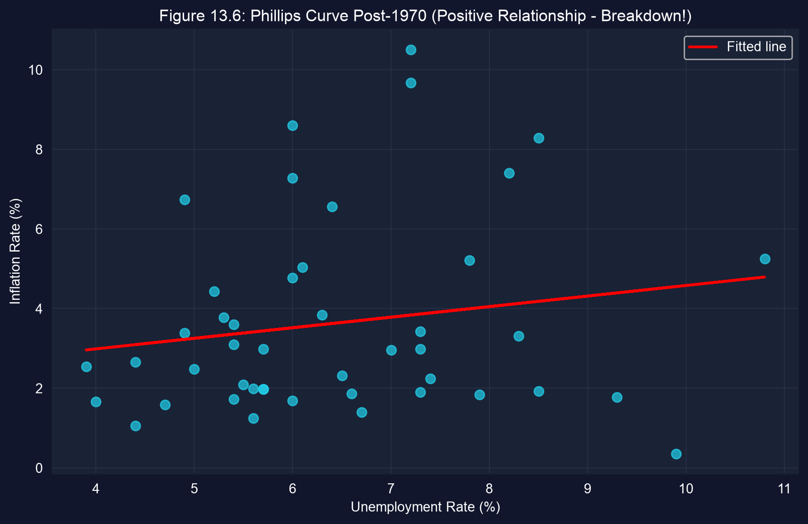
Same two variables, opposite sign. Either the economy changed, or the bivariate model was always missing something.

Key Concept 13.4. Be precise: the slope flips sign, but we cannot reject a zero relationship (95% CI from −0.39 to +0.92). Stagflation shows up as points with high unemployment and high inflation. The Friedman–Phelps answer: the missing piece is expected inflation.

The OVB formula: what an omitted regressor does to a slope

\[\underbrace{y = \beta_1 + \beta_2 x + \beta_3 z + u}_{\text{long (true) model}} \qquad \underbrace{z = \gamma_1 + \gamma\,x + v}_{\text{auxiliary regression}}\]

Substitute \(z\) into the long model and regress \(y\) on \(x\) alone:

\[E[b_2] = \beta_2 + \underbrace{\beta_3\,\gamma}_{\text{omitted variables bias}}\]

The bias is (effect of the omitted \(z\) on \(y\)) × (how \(z\) moves with the included \(x\)). It vanishes only if \(\beta_3 = 0\) or \(\gamma = 0\).

Key Concept 13.5. Direction of the bias: sign(β₃) × sign(γ). If z raises y (β₃ > 0) and rises with x (γ > 0), the short slope is biased upward, and enough upward bias can turn a negative true slope positive. With OLS on the same sample, the in-sample version b₂(short) = β̂₂ + β̂₃·γ̂ holds exactly, not just in expectation.

Code: add expected inflation, then run the auxiliary regression

# continues from the previous block
data_exp = data_post1970.dropna(subset=["inflgdp1yr"]).copy()  # rows with expected inflation
data_exp["_time"] = range(len(data_exp))                       # time index for HAC
fit_augmented = pf.feols("inflgdp ~ urate + inflgdp1yr", data=data_exp,
                         vcov="NW", vcov_kwargs={"time_id": "_time", "lag": 5})  # long model
fit_aux = pf.feols("inflgdp1yr ~ urate", data=data_exp)        # auxiliary: z on x
beta2 = fit_augmented.coef()["urate"]       # true slope on unemployment
beta3 = fit_augmented.coef()["inflgdp1yr"]  # effect of expected inflation
gamma = fit_aux.coef()["urate"]             # how expectations co-move with unemployment
print(beta2 + beta3 * gamma, fit_post.coef()["urate"])  # predicted vs actual short slope

↗ Try it in Colab

inflgdp1yr is one-year-ahead expected inflation from the Survey of Professional Forecasters. It is available for all 45 post-1970 years, so the long, short and auxiliary regressions use the same sample, which is what makes the decomposition exact.

Output: control for expectations and the negative slope returns

Variable (long model)	Coef.	HAC SE	\(t\)	\(p\)	95% CI
Intercept	0.270	0.634	0.43	0.672	[−1.01, 1.55]
urate (\(\hat\beta_2\))	−0.128	0.081	−1.58	0.122	[−0.29, 0.04]
inflgdp1yr (\(\hat\beta_3\))	1.146	0.085	13.48	< 0.001	[0.97, 1.32]

N = 45 · NW, 5 lags · \(R^2 = 0.881\) · Auxiliary regression: \(\hat\gamma = 0.343\) (SE 0.195, \(p = 0.086\), default SEs)

Expected inflation does most of the work (\(R^2\) jumps from 0.03 to 0.88), and the unemployment slope turns negative again.

β̂₃ ≈ 1.15: actual inflation moves roughly one-for-one with expected inflation (the chapter’s “coefficient ≈ 1”; we have not formally tested β₃ = 1). β̂₂ = −0.128 has the Phillips-curve sign but is not significant at 5% (p = 0.12), so the trade-off is restored in sign, not firmly established. γ̂ = 0.343: years with higher unemployment also had higher expected inflation.

The OVB arithmetic explains the sign reversal exactly

\[b_2^{\text{short}} = \hat\beta_2 + \hat\beta_3\,\hat\gamma = -0.128 + 1.146 \times 0.343 = +0.265\]

Piece	Value	Meaning
\(\hat\beta_2\)	−0.128	unemployment slope, holding expectations fixed
\(\hat\beta_3\hat\gamma\)	+0.393	bias from omitting expected inflation
\(b_2^{\text{short}}\)	+0.265	the bivariate post-1970 slope: an exact match

The bivariate slope gave unemployment credit for expected inflation’s effect. The bias (+0.39) was large enough to flip the sign.

The chapter calls this a “perfect match”. It is perfect by construction: for OLS on a common sample the decomposition is an algebraic identity. Its value is in attributing the short slope: −0.128 of genuine trade-off plus +0.393 of omitted-variable bias. Economic story: 1970s supply shocks (oil) raised unemployment and inflation expectations together, so γ > 0; and expectations push inflation up (β₃ > 0); so the bias is positive.

Caveats: the trade-off is restored in sign, not proven

• Imprecision: the augmented slope (\(-0.128\), \(p = 0.12\)) and \(\hat\gamma\) (\(p = 0.086\)) are not significant at 5%
• Measurement: expected inflation is a forecasters’ survey, a proxy for what wage- and price-setters actually expected
• Simultaneity: inflation and unemployment are both outcomes of the same shocks and policies, so this is not a causal structural equation
• Other omitted variables: supply shocks and policy regimes can still bias the long model

The OVB formula is a diagnostic: it tells us the direction and size of the bias from a named omitted variable. It cannot rule out the omitted variables we have not named.

The chapter itself notes the post-1970 slope (p ≈ 0.42) and the augmented urate coefficient (p ≈ 0.12) are not significant. The broader lesson for the policy debate: once expectations adjust, there is little long-run trade-off to exploit, which is why central banks focus on anchoring expectations.

Case 13.4 · What determines fuel economy?

Log-log model · 26,995 vehicles · cluster-robust standard errors

Case 13.4: a large cross-section of vehicles. Tools: elasticities from a log-log model, and why grouped data need cluster-robust standard errors.

The question: why didn’t fuel economy improve more?

Data. 26,995 vehicle models sold in the U.S., 1980–2006, from 39 manufacturers (AED_AUTOSMPG.DTA). The logs come pre-computed in the data.

• mpg: miles per gallon (8.7 to 76.4)
• curbwt: weight in pounds (1,450 to 6,700)
• hp, torque: engine power and pulling force
• year: model year (a technology trend)
• mfr: manufacturer (the clustering variable)

Top manufacturers	Models
GMC	7,979
Chrysler	4,172
Ford	3,709
Toyota	1,554
Nissan	1,079
Volkswagen	831
Honda	743

Engines kept improving, so where did the efficiency gains go? This case links fuel economy to vehicle attributes.

Policy context: post-oil-shock demand for efficiency, CAFE fuel-economy standards, the rise of SUVs and trucks, and steady engine technology. Observations are model-level records, not sales-weighted. The panel is very unbalanced across manufacturers: GMC alone has 7,979 rows (about 30%), and the average is about 692 per manufacturer.

After 1985, the gains went into power, not mileage

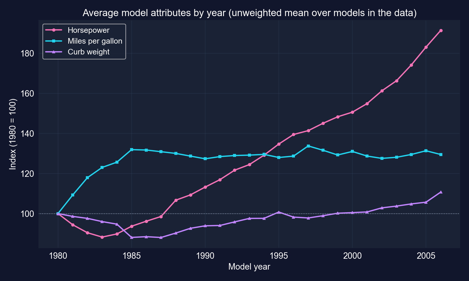
Unweighted average over the models in the data, indexed to 1980 = 100. Average MPG rose about 32% by 1985, then stayed roughly flat while horsepower nearly doubled.

From 1985 to 2006, average horsepower climbed steadily while average MPG barely moved.

Slide-only figure built from the same data (simple means by model year). 1980 → 2006: mpg 19.4 → 25.2 (index 129.5), hp 126.5 → 242.3 (index 191.5), weight 3,517 → 3,894 lb (index 110.7). These are not sales-weighted fleet averages, so read them as the attributes of the models on offer.

Why cluster by manufacturer?

Vehicles from the same manufacturer share engine platforms, engineering teams, design philosophy and testing practices. So their regression errors are correlated within the manufacturer.

Default / HC1 SEs assume

• 26,995 independent pieces of information
• Too-small SEs, too-large \(t\)-stats

Cluster-robust (CRV1) SEs allow

• any correlation inside each of the 39 manufacturers
• independence only across manufacturers

With correlated errors, the effective sample size is closer to the number of clusters than to the number of rows.

Key Concept 13.6. Ignoring within-cluster correlation understates uncertainty and leads to false rejections. CRV1 is pyfixest’s standard cluster-robust estimator with a small-sample correction.

Code: log-log regression with SEs clustered by manufacturer

!pip install -q pyfixest                    # pyfixest is not preinstalled in Colab
import pandas as pd                         # tabular data
import pyfixest as pf                       # OLS with R-style formulas
url = "https://raw.githubusercontent.com/quarcs-lab/data-open/master/AED/AED_AUTOSMPG.DTA"
data_auto = pd.read_stata(url)              # 26,995 vehicles, 1980–2006 (logs pre-computed)
print(data_auto[["mpg", "curbwt", "hp", "torque", "year"]].describe())  # summary statistics
print(data_auto["mfr"].value_counts().head(10))                       # observations per maker
# log MPG on log HP, log weight, log torque and a linear year trend
fit_auto = pf.feols("lmpg ~ lhp + lcurbwt + ltorque + year", data=data_auto,
                    vcov={"CRV1": "mfr"})   # cluster-robust SEs by manufacturer
fit_auto.summary()                          # elasticities + clustered SEs
print(data_auto["mfr"].nunique())           # number of clusters: 39

↗ Try it in Colab

Self-contained. The dataset already contains lmpg, lhp, lcurbwt and ltorque. The year enters in levels, so its coefficient is a proportional change in MPG per model year, holding the engine and weight fixed.

Output: weight is the dominant determinant of fuel economy

Variable	Coef.	CRV1 SE	\(t\)	\(p\)	95% CI
Intercept	−20.843	1.988	−10.48	< 0.001	[−24.87, −16.82]
lhp	−0.181	0.065	−2.79	0.008	[−0.31, −0.05]
lcurbwt	−0.562	0.057	−9.94	< 0.001	[−0.68, −0.45]
ltorque	−0.141	0.064	−2.21	0.033	[−0.27, −0.01]
year	0.0152	0.0011	13.84	< 0.001	[0.013, 0.017]

N = 26,995 · SEs clustered by manufacturer (39 clusters) · \(R^2 = 0.777\)

Weight carries the largest elasticity, and the year trend shows steady technical progress at fixed attributes.

The model explains 78% of the variation in log MPG; the rest reflects aerodynamics, transmissions, fuel type and so on. Note the CI uses the cluster-robust SE with G − 1 = 38 degrees of freedom.

Reading the elasticities: technology was “spent” on weight and power

• Weight −0.56: a 1% heavier vehicle gets ≈ 0.56% lower MPG, holding power, torque and year fixed (the largest effect)
• Horsepower −0.18 and torque −0.14: ≈ 0.18% and ≈ 0.14% lower MPG per 1% increase
• Year +0.0152: at fixed weight, power and torque, MPG rises about 1.5% per model year (\(100 \times (e^{0.0152}-1) = 1.53\%\))
• The paradox resolved: the technology trend kept raising MPG at given attributes, while rising horsepower and weight pulled it back down

Engineers made engines more efficient every year, and buyers took the gains as more powerful (and somewhat heavier) cars.

All elasticity statements are approximations for small changes (log-log model). The year coefficient is a semi-elasticity: 100 × 0.0152 ≈ 1.52% is the approximation; the exact proportional change is 1.53%. Policy relevance from the chapter: weight matters a great deal for CAFE compliance; lighter materials and smaller turbocharged engines are later responses (after the data end).

Clustering makes the standard errors 6–9× larger

Variable	HC1 SE (ignores clusters)	CRV1 SE (by manufacturer)	Ratio
lhp	0.0071	0.0651	9.1×
lcurbwt	0.0080	0.0566	7.0×
ltorque	0.0076	0.0640	8.4×
year	0.00017	0.0011	6.4×

Same coefficients; only vcov changes. HC1 comparison: pf.feols("lmpg ~ lhp + lcurbwt + ltorque + year", data=data_auto, vcov="HC1")

If we ignored the clustering, every \(t\)-statistic would be inflated 6–9×. The torque effect (\(t = 2.21\) clustered) would look like \(t \approx 18.6\).

This comparison is computed for the slides (same model, same data, only the vcov differs) to quantify the chapter’s statement that clustering increases the SEs. Errors within a manufacturer are strongly correlated, so the 26,995 rows contain far less independent information than their number suggests. HC1 t for ltorque: −0.1415 / 0.0076 ≈ −18.6.

Caveats: an engineering association, not a causal effect

• Joint choices: weight, power and torque are chosen together by designers, so “a 1% heavier car, all else equal” is a comparison across models, not an experiment
• Few, unbalanced clusters: 39 manufacturers, and GMC alone is about 30% of the rows. Cluster-robust inference works best with many similar-sized clusters
• Not sales-weighted: every model counts equally, regardless of how many units sold
• Overlapping engine measures: horsepower and torque capture related engine traits, which blurs their separate effects

Within these limits, the large weight elasticity and the year trend are robust, and they tell a coherent story.

Standard caveats. With few or very unequal clusters, CRV1 SEs can still be too small; wild-cluster bootstrap is the usual remedy (not covered here). The chapter’s Key Takeaways list 13.4 under “Advanced Causal Methods”, but this is an observational, descriptive regression: a tool case (clustering), not a design for causation.

Act II-b · Four designs that identify causation

Cases 13.5–13.8 · RCT · DiD · RD · IV

From here on, each case asks a causal question, and each answers it with a design that supplies a credible counterfactual. The estimator is still OLS (or 2SLS); what changes is why we believe the slope.

Why a raw comparison is not a causal effect

\[\underbrace{E[Y \mid D{=}1] - E[Y \mid D{=}0]}_{\text{observed difference}} = \underbrace{E[Y_1 - Y_0 \mid D{=}1]}_{\text{effect on the treated (ATT)}} + \underbrace{E[Y_0 \mid D{=}1] - E[Y_0 \mid D{=}0]}_{\text{selection bias}}\]

\(Y_1\), \(Y_0\): potential outcomes with and without treatment. We only ever observe one of them per unit. The other is the counterfactual.

Every design in this act is a strategy for driving the selection-bias term to zero.

Selection bias is the difference the treated and untreated would have shown even without treatment. In observational data it is generally non-zero: people who buy generous insurance expect to need care; parties that win were already strong; rich countries can afford good institutions. This is the potential-outcomes way of saying “confounding”.

Four ways to build the counterfactual

Design	Where the counterfactual comes from	Case
RCT	a randomly assigned control group	13.5 RAND health insurance
Difference-in-differences	the control group’s change over time	13.6 South African clinics
Regression discontinuity	units just on the other side of a cutoff	13.7 Senate elections
Instrumental variables	variation in treatment driven only by an instrument	13.8 colonial institutions

Each design swaps the unverifiable “I controlled for everything” for one specific assumption you can argue about.

Keep this table in mind; the synthesis at the end of the deck adds the identifying assumption, the estimand and the main threat for each.

Case 13.5 · Does cost-sharing reduce medical spending?

Randomized controlled trial · RAND Health Insurance Experiment · SEs clustered by family

Case 13.5: the gold standard. Tools: regression on treatment dummies, a joint F-test with cluster-robust covariance, and the logic of random assignment.

The question: does cheaper care mean more care?

Moral hazard: if insurance makes care cheaper at the point of use, do people use more of it? That question drives every debate about deductibles and co-pays.

Why observational data fail. People choose their insurance:

• those who expect to be sick buy more generous plans
• income, education and health all affect both plan choice and spending

In observational data, “generous plan → higher spending” mixes the plan’s effect with who chose it.

Reverse causation too: health status affects insurance choice. Comparing spending across self-chosen plans therefore estimates the effect plus selection bias, with no way to separate them.

The design: random assignment to insurance plans

RAND Health Insurance Experiment (1974–1982)

• families randomly assigned to plans
• coinsurance (the share of the bill you pay): 0% (free care), 25%, mixed 25/50%, 50%, 95%, or an individual deductible
• followed for 3–5 years

Why it works

• assignment is independent of health, income and preferences
• so the groups are identical in expectation
• selection bias \(= 0\) in expectation, so the difference in means estimates the causal effect of each plan vs free care

Randomization does not equalize the groups exactly. It makes every difference before treatment pure chance, which standard errors already account for.

Key Concept 13.7. Estimand: the average effect, among experiment participants, of being assigned to plan j rather than free care. Because families (not individuals) were assigned, outcomes of members of the same family are correlated, hence SEs clustered by family.

The data: year 1 of the experiment

	Value
Person-year observations, all years	20,203
Observations used (year 1 only)	5,639
Families (clusters) in year 1	1,930
Median annual spending (2011 $)	$479
Largest annual spending	$175,831

Outcome spending = inpatient + outpatient medical spending in 2011 dollars. Plan dummies: coins25, coinsmixed, coins50, coins95, coinsindiv; free care is the omitted baseline.

Spending is extremely skewed (median $479, maximum $175,831), so group means will be noisy.

The chapter follows the textbook and uses year 1 only. The heavy right tail (a few very expensive hospitalizations) is why some plan means are imprecise, especially in smaller groups.

Code: load the experiment and compare mean spending by plan

!pip install -q pyfixest                    # pyfixest is not preinstalled in Colab
import pandas as pd                         # tabular data
import pyfixest as pf                       # OLS with R-style formulas
url = "https://raw.githubusercontent.com/quarcs-lab/data-open/master/AED/AED_HEALTHINSEXP.DTA"
data_health = pd.read_stata(url)            # RAND HIE, all years (20,203 person-years)
data_health_y1 = data_health[data_health["year"] == 1]   # first year only: 5,639 obs
spending_by_plan = data_health_y1.groupby("plan")["spending"].agg(["mean", "std", "count"])
print(spending_by_plan)                     # mean, SD and size of each randomized group

↗ Try it in Colab

With random assignment, this simple table of group means is already a causal comparison.

Self-contained. groupby(“plan”) gives one row per randomized arm. Note the standard deviations: the 50% plan has SD ≈ $11,644, about three times its neighbours, because of a few huge spenders.

Output: free care has the highest spending

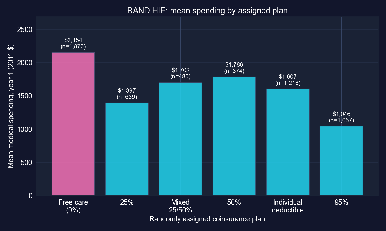
Mean year-1 spending by randomly assigned plan (2011 $), with group sizes.

Every cost-sharing plan spends less than free care, and the 95% plan spends about half.

Slide-only figure from the chapter’s group means: free care $2,154 (n = 1,873); 25% $1,397 (639); mixed $1,702 (480); 50% $1,786 (374); individual deductible $1,607 (1,216); 95% $1,046 (1,057). The ordering is not perfectly monotone in the coinsurance rate (50% > 25%): the next slides show the 50% group is too noisy to rank.

Code: the RCT regression with SEs clustered by family

# continues from the previous block
# spending on plan dummies; free care (coins0) is the omitted baseline
fit_rct = pf.feols("spending ~ coins25 + coins50 + coins95 + coinsmixed + coinsindiv",
                   data=data_health_y1, vcov={"CRV1": "idfamily"})  # cluster by family
fit_rct.summary()                           # each coefficient = plan mean − free-care mean

↗ Try it in Colab

A regression on a full set of group dummies reproduces the group means exactly: intercept = baseline mean, slopes = differences from it.

Check: intercept 2,153.57 = free-care mean; 2,153.57 − 1,107.75 = 1,045.82 = 95% plan mean. The regression adds clustered standard errors and a framework for joint tests.

Output: most cost-sharing plans cut spending significantly

Variable	Coef. ($)	CRV1 SE	\(t\)	\(p\)	95% CI	% of baseline
Intercept (free care)	2,153.57	118.31	18.20	< 0.001	[1,921.5, 2,385.6]	—
coins25	−756.91	190.04	−3.98	< 0.001	[−1,129.6, −384.2]	−35%
coins50	−367.72	618.04	−0.59	0.552	[−1,579.8, 844.4]	−17%
coins95	−1,107.75	150.37	−7.37	< 0.001	[−1,402.6, −812.9]	−51%
coinsmixed	−451.70	239.42	−1.89	0.059	[−921.3, 17.9]	−21%
coinsindiv	−546.50	162.15	−3.37	< 0.001	[−864.5, −228.5]	−25%

Plans: coins25 25% · coins50 50% · coins95 95% · coinsmixed 25/50% · coinsindiv individual deductible · N = 5,639 · SEs clustered by family (1,930) · \(R^2 = 0.007\)

Three plans are clearly below free care. The 50% plan is not significantly different (\(p = 0.55\)): its CI runs from \(-\$1{,}580\) to \(+\$844\).

Percent column = coefficient / free-care mean. The 50% plan’s huge SE (618 vs 150–240 for the others) comes from its small size (374) and extreme outliers (SD ≈ $11,644). Mixed 25/50% is borderline (p = 0.059). Report the imprecise estimates honestly rather than saying “all plans reduce spending”.

Code + output: do the plans matter jointly?

# continues from the previous block
import numpy as np                          # matrix algebra
from scipy.stats import f as f_dist         # F distribution
coef_names = ["coins25", "coins50", "coins95", "coinsmixed", "coinsindiv"]
coefs = np.array([fit_rct.coef()[c] for c in coef_names])        # the 5 plan effects
idx = [list(fit_rct.coef().index).index(c) for c in coef_names]  # their positions
V_sub = fit_rct._vcov[np.ix_(idx, idx)]     # clustered covariance of the 5 effects
f_val = coefs @ np.linalg.inv(V_sub) @ coefs / len(coef_names)   # Wald F statistic
p_val = 1 - f_dist.cdf(f_val, len(coef_names), fit_rct._N - len(fit_rct.coef()))
print(f_val, p_val)                         # H0: all five plan effects = 0

↗ Try it in Colab

Result: \(F = 11.39\), \(p < 0.001\). We reject that insurance generosity is irrelevant: plan design causally changes spending.

H0: all five plan coefficients are zero (no plan differs from free care). F(5, 5,633) = 11.39, p ≈ 6 × 10⁻¹¹. The Wald statistic uses the cluster-robust covariance matrix, so the joint test is consistent with the clustered SEs.

Interpretation: moral hazard is real, and moderate

• Causal reading: because plans were randomized, the −$1,108 for the 95% plan is the effect of facing 95% coinsurance instead of free care, about 51% less spending in year 1
• Magnitude: cost-sharing cuts spending by roughly a quarter to a half, depending on the plan; that is meaningful but not dramatic
• \(R^2 = 0.007\) is irrelevant to causality: individual health shocks drive most of the spending variation. A low \(R^2\) means we predict individuals poorly, not that the effect is biased
• Policy: free care raises use; cost-sharing lowers costs but may also cut necessary care

An RCT turns a difference in means into a causal effect. Precision, not bias, is the remaining problem.

The chapter says the low R² “is actually good”. The more precise statement is that R² is irrelevant for identifying a causal effect: randomization guarantees unbiasedness regardless of R²; a low R² only implies that the outcome has a lot of other variation. The RAND results shaped U.S. health-insurance design (Medicare/Medicaid cost-sharing, later ACA debates).

Threats to an RCT: what can still go wrong

• Attrition: if families who dislike their plan drop out (more likely under heavy cost-sharing), the remaining groups are no longer comparable
• Non-compliance and refusal at enrollment can undo the balance that randomization created
• Balance check (not run in the chapter): compare baseline age, income and health across plans; they should differ only by chance
• External validity: six U.S. sites in the 1970s; health care has changed since
• Ethics and cost: randomizing insurance is rarely possible, which is why the next three designs exist

Randomization identifies the effect for the people in the experiment. Its credibility then depends on keeping the randomized groups intact.

Standard RCT caveats. Aron-Dine, Einav and Finkelstein (2013, Journal of Economic Perspectives) revisit the RAND experiment and discuss differential attrition and refusal across plans. The dataset includes baseline covariates (age, famincome, educ, health status), so a balance table is an easy exercise.

Case 13.6 · Did free care improve child nutrition?

Difference-in-differences · South Africa, 1993 vs 1998 · SEs clustered by community

Case 13.6: no randomization, but a before/after comparison between more- and less-exposed communities. Tools: the 2×2 DiD table, the interaction regression, and the parallel-trends assumption.

The question: did the 1994 health reform improve child nutrition?

• The policy (1994): post-apartheid South Africa made public primary care free for young children and pregnant women (studied by Tanaka 2014)
• Who could benefit: free care helps only if a clinic is within reach
• Treatment group: children in communities that had a clinic in 1993 (hightreat = 1); comparison group: children in communities without one
• Outcome: waz, the weight-for-age \(z\)-score, a standard measure of child nutrition

Exposure to the reform depended on where a child lived, which gives a natural treatment and comparison group.

Data: AED_HEALTHACCESS.DTA, 1,071 children aged 0–4 in rural KwaZulu-Natal, surveyed in 1993 (before) and 1998 (after), 54 communities; source Tanaka (2014, AEJ: Economic Policy). The dataset labels hightreat as “= 1 if community has clinic in 1993”. (The chapter narrates this as “communities that got many new clinics”; the slides follow the dataset label and the source paper: treatment intensity is pre-existing clinic access to the newly free care.) Note the children in 1993 and 1998 are different children (two cohorts aged 0–4), not the same children followed over time.

The design: difference out both the level gap and the common trend

Group	1993 (pre)	1998 (post)	Change
High treatment (clinic)	\(\bar Y_{T,0}\)	\(\bar Y_{T,1}\)	\(\Delta_T\)
Low treatment (no clinic)	\(\bar Y_{C,0}\)	\(\bar Y_{C,1}\)	\(\Delta_C\)

\[\text{DiD} = (\bar Y_{T,1} - \bar Y_{T,0}) - (\bar Y_{C,1} - \bar Y_{C,0}) = \Delta_T - \Delta_C\]

The first difference removes permanent gaps between communities. The second removes changes common to everyone (national trends, the economy).

Key Concept 13.8. Identifying assumption, parallel trends: without the reform, the treated communities’ mean waz would have changed by the same amount as the comparison communities’ (Δ_C). Estimand: the average effect on the treated (ATT), meaning children in communities with clinic access.

Code: the 2×2 table of means and the DiD by hand

!pip install -q pyfixest                    # pyfixest is not preinstalled in Colab
import pandas as pd                         # tabular data
import pyfixest as pf                       # OLS with R-style formulas
url = "https://raw.githubusercontent.com/quarcs-lab/data-open/master/AED/AED_HEALTHACCESS.DTA"
data_access = pd.read_stata(url)            # 1,071 children aged 0–4; 1993 and 1998
print(data_access.groupby(["hightreat", "post"])["waz"].agg(["mean", "count"]))  # 2×2 means
m = data_access.groupby(["hightreat", "post"])["waz"].mean()  # the four cell means
pre_control, post_control = m[(0, 0)], m[(0, 1)]   # no clinic: 1993, 1998
pre_treat, post_treat = m[(1, 0)], m[(1, 1)]       # clinic: 1993, 1998
did_estimate = (post_treat - pre_treat) - (post_control - pre_control)
print(post_control - pre_control, post_treat - pre_treat, did_estimate)  # ΔC, ΔT, DiD

↗ Try it in Colab

Self-contained and equivalent to the chapter’s code (which computes each cell mean with a boolean filter). hightreat and post are 0/1 indicators; postXhigh = post × hightreat is also in the data.

Output: the treated group improved by 0.52 more

Mean waz (n)	1993 (pre)	1998 (post)	Change
Low treatment (no clinic)	−0.414 (325)	−0.069 (288)	+0.345
High treatment (clinic)	−0.545 (246)	0.321 (212)	+0.867
Difference (high − low)	−0.131	+0.391	+0.522

DiD \(= 0.867 - 0.345 = 0.522\). The same number appears as the difference of the two columns: \(0.391 - (-0.131) = 0.522\).

Children in clinic communities started slightly behind, ended clearly ahead, and gained 0.52 more than the comparison group.

Both groups improved (child nutrition was improving everywhere). The comparison group’s +0.345 is our estimate of what would have happened to the treated group without the reform. Subtracting it leaves 0.522.

Naive vs design: two shortcuts, two different biases

Comparison	Estimate	What it gets wrong
After-only gap (1998: high − low)	0.391	ignores that treated children started 0.131 lower, so it is biased down
Before–after, treated only	0.867	credits the reform with the common improvement (+0.345), so it is biased up
Difference-in-differences	0.522	removes both the baseline gap and the common trend

Each single difference is contaminated by one confounder. Using both differences removes both.

Both naive numbers come straight from the 2×2 table (no new estimation). The before–after estimate (0.867) is 66% larger than DiD; the post-only gap (0.391) is 25% smaller. This is the “OLS vs design” thread: the naive comparisons are what you would report without a design.

Code: DiD as a regression with an interaction term

# continues from the previous block
# waz on group, period and their interaction (postXhigh = post × hightreat)
fit_did = pf.feols("waz ~ hightreat + post + postXhigh", data=data_access,
                   vcov={"CRV1": "idcommunity"})   # cluster by community (54 clusters)
fit_did.summary()                           # postXhigh = the DiD estimate
print(fit_did.coef()["postXhigh"], did_estimate)   # identical: 0.522 and 0.522

↗ Try it in Colab

The regression gives the same 0.522, plus a standard error that accounts for correlation within communities.

Treatment varies at the community level, and children in the same community share unobserved shocks, so we cluster by community. The regression form also extends naturally to covariates and more periods.

Output: every coefficient is one cell of the 2×2 table

Variable	Coef.	CRV1 SE	\(t\)	\(p\)	95% CI	= in the 2×2 table
Intercept	−0.414	0.115	−3.60	0.001	[−0.645, −0.183]	control, 1993
hightreat	−0.131	0.197	−0.67	0.508	[−0.526, 0.264]	baseline gap
post	0.345	0.137	2.52	0.015	[0.070, 0.620]	common trend (\(\Delta_C\))
postXhigh	0.522	0.235	2.22	0.031	[0.050, 0.994]	DiD

N = 1,071 · SEs clustered by community (54 clusters) · \(R^2 = 0.040\)

The baseline gap is small and insignificant (\(p = 0.51\)), and the DiD effect is significant at 5% (\(p = 0.031\)), though its CI is wide.

Reading guide: intercept = control-group pre mean; hightreat = treated − control in 1993; post = control change 1993→1998; postXhigh = extra change for the treated. The insignificant baseline gap is reassuring (groups looked similar before the reform) but is not a test of parallel trends.

The counterfactual: where the treated group would have been

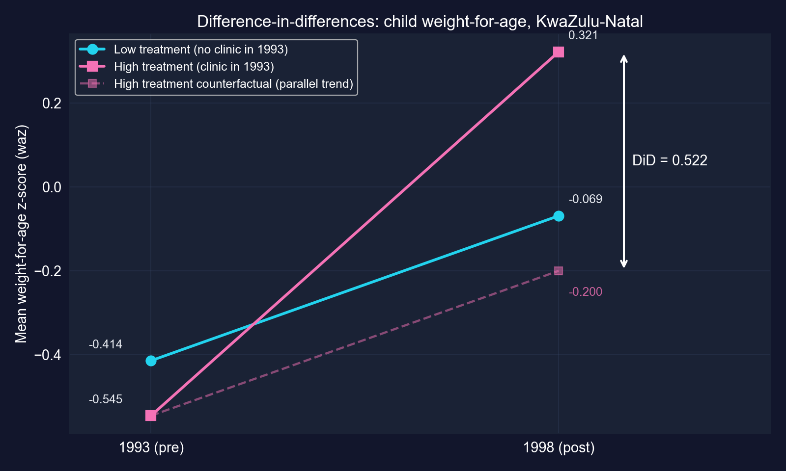
Mean waz by group and year. Dashed: the treated group’s counterfactual path under parallel trends (−0.545 + 0.345 = −0.200).

The effect is the vertical gap between what happened (0.321) and the parallel-trend counterfactual (−0.200), which is 0.522.

Slide-only figure built from the four cell means. The dashed line is the assumption made visible: it borrows the comparison group’s slope. If the treated communities were already on a steeper path, the dashed line is wrong and so is the estimate.

Interpretation: a large effect, imprecisely measured

• Units: waz is measured in SDs of a reference growth standard, so the effect is +0.52 \(z\)-units. In this sample waz has SD 1.59, so that is about 0.33 sample SDs
• Significance: \(p = 0.031\), so we reject “no effect” at 5%
• Precision: the 95% CI is [0.05, 0.99]; the data support anything from a negligible to a very large effect
• Causal claim: the reform’s effect on children in clinic communities, if parallel trends hold

DiD gives a credible direction and a plausible magnitude. With 54 communities, the precision is modest.

The chapter says 0.52 “SD”, but z-scores are standardized against a reference population, not this sample; relative to this sample’s dispersion (SD 1.59) the effect is about a third of an SD, still substantial. The chapter’s translations (e.g. “25th to 45th percentile”, “6–12 months of growth”) assume a unit-SD distribution and are not computed from the data, so they are not repeated here. Low R² (0.04) is irrelevant to identification.

Threats: parallel trends cannot be tested with two periods

• Untestable here: with one pre-period we cannot check whether the groups were trending together before 1994 (more pre-periods allow an event-study check)
• Different places: communities with clinics may differ (roads, water, income) and could have improved faster anyway
• Concurrent changes: other post-1994 programs that favored clinic communities would be counted as the reform’s effect
• Changing composition: different children are measured in 1993 and 1998; if who lives in treated communities changed, so does the mean
• Inference: 54 clusters, so CRV1 SEs are reasonable but not exact

Every DiD estimate rests on the dashed line. Defend it with institutional knowledge, pre-trends and placebo tests.

Standard DiD threats. The source study (Tanaka 2014) reports falsification exercises: no pre-existing trend before the reform, and no effect among children who were not eligible. These are not run in the chapter. The chapter’s evidence-for-validity list (“placement based on need”, “no other programs”) is asserted rather than shown in the data.

Case 13.7 · Do parties gain from holding a Senate seat?

Regression discontinuity · U.S. Senate elections, 1914–2010 · HC1 standard errors

Case 13.7: a sharp cutoff (50% of the vote decides who wins) creates as-good-as-random variation in incumbency for close races. Tools: running variable, cutoff, the RD regression, and the locality of the estimate.

The question: is there an incumbency advantage?

Parties that hold a seat tend to win it again. But is that because holding the seat helps, or because parties that win were stronger to begin with?

The data (AED_INCUMBENCY.DTA): 1,390 U.S. Senate elections, 1914–2010

• margin: Democratic margin of victory in election \(t\) (percentage points, −100 to +100)
• win \(= 1\) if margin \(> 0\) (the Democrat won the seat)
• vote: Democratic vote share in the next election for that seat, \(t+1\) (1,297 non-missing)

The unit is the party’s seat, so this case measures the party incumbency advantage: the gain to the Democratic party from having won the seat last time.

The chapter phrases the question as a candidate’s incumbency advantage. The dataset’s labels show the outcome is the Democratic party’s vote share in the next election, and the running variable is the Democratic margin in election t, so the estimand is the party-level incumbency effect (as in Lee 2008’s House study). The candidate may or may not run again.

The design: compare races that were barely won with races that were barely lost

• Running variable: margin
• Cutoff: margin \(= 0\)
• Treatment: winning, which switches on sharply at the cutoff
• Key assumption, continuity: without the treatment, average outcomes would vary smoothly through the cutoff

\[\text{vote}_{t+1} = \beta_1 + \beta_2\,\text{win}_t + \beta_3\,\text{margin}_t + u\]

\(\beta_2\) is the jump in the outcome at margin \(= 0\), after controlling for the smooth effect of the margin.

Within a hair of 50%, who wins is close to a coin flip, so winners and losers are comparable except for winning.

Key Concept 13.9. Estimand: the effect of winning at the cutoff, i.e. for close races. It is local by construction. The chapter’s specification imposes one common slope on both sides of the cutoff and uses every election, whatever its margin.

Naive vs design: comparing all winners with all losers is badly biased

Comparison	Next-election Democratic vote share	Gap
Seats the Democrats won (702)	62.6%
Seats the Democrats lost (595)	40.9%
Naive difference		21.7 pp
RD estimate at the cutoff (next slides)		4.8 pp

Most of the raw 21.7-point gap is selection: states where Democrats win comfortably will keep voting Democratic, incumbent or not.

Naive gap = simple difference in mean vote between win = 1 and win = 0 races (same 1,297 observations; computed for the slides). The RD estimate is less than a quarter of it. This is the selection bias the design removes.

Code: the RD regression

!pip install -q pyfixest                    # pyfixest is not preinstalled in Colab
import pandas as pd                         # tabular data
import pyfixest as pf                       # OLS with R-style formulas
url = "https://raw.githubusercontent.com/quarcs-lab/data-open/master/AED/AED_INCUMBENCY.DTA"
data_incumb = pd.read_stata(url)            # 1,390 Senate elections, 1914–2010
print(data_incumb[["vote", "margin", "win"]].describe())   # running variable and outcome
data_rd = data_incumb[data_incumb["vote"].notna()].copy()  # keep races with a t+1 outcome
naive = data_rd.groupby("win")["vote"].mean()               # naive: winners vs losers
fit_rd = pf.feols("vote ~ win + margin", data=data_rd, vcov="HC1")  # jump + linear margin
fit_rd.summary()                            # win coefficient = discontinuity at 0
print(fit_rd.confint().loc["win"])          # 95% CI for the jump

↗ Try it in Colab

Self-contained. Line 8 adds the naive comparison used on the previous slide; the rest is the chapter’s code. 93 races have no next-election outcome and are dropped (1,390 → 1,297).

Output: barely winning adds about 4.8 percentage points next time

Variable	Coef.	HC1 SE	\(t\)	\(p\)	95% CI
Intercept	47.331	0.526	89.95	< 0.001	[46.30, 48.36]
win	4.785	0.860	5.56	< 0.001	[3.10, 6.47]
margin	0.348	0.017	20.42	< 0.001	[0.315, 0.381]

N = 1,297 · HC1 SEs · \(R^2 = 0.578\)

• Barely lost (margin \(\to 0^-\)): predicted next-time Democratic share 47.3%
• Barely won (margin \(\to 0^+\)): 47.3 + 4.8 = 52.1%
• Each extra point of margin today: +0.35 points next time (on both sides, by assumption)

The jump at the cutoff is 4.8 percentage points, not 4.8%, and it is precisely estimated.

The outcome is a vote share in percent, so the effect is in percentage points. “4.8%” would mean a 4.8% proportional increase, which is a different and wrong statement. 95% CI: 3.1 to 6.5 pp.

The discontinuity, visualized

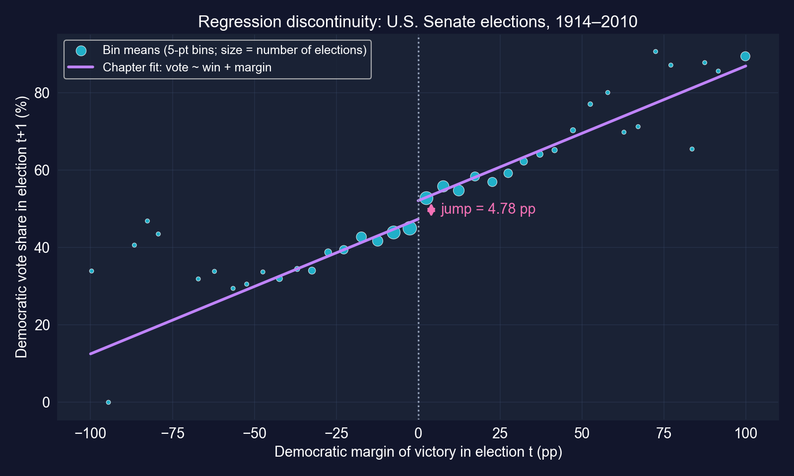
Binned means of next-election Democratic vote share by current margin (5-point bins). Purple: the chapter’s fitted model, one slope, with a jump at 0.

The bins jump at zero: races just won sit visibly above races just lost.

Slide-only figure; the chapter describes this plot but shows only ASCII art. Bin size scales with the number of elections; most races are within ±25 points. The single straight line with a common slope fits the middle well but misses the extremes (e.g. uncontested races at ±100), which motivates the robustness discussion.

Interpretation: a local, party-level causal effect

• Causal because near margin \(= 0\), winning is as-good-as random: barely-winning and barely-losing parties face similar states, candidates and conditions
• Local: it applies to close races, not to landslides; the advantage in safe seats is not identified
• Party-level: the Democratic party’s seat-holding advantage, whether or not the same senator runs again
• Mechanisms (not separated here): name recognition, fundraising, media access, constituent service

RD trades breadth for credibility: a very believable effect, for a narrow set of elections.

Selection bias is removed only at the cutoff; away from it, winners and losers differ systematically (as the naive 21.7 shows). The chapter’s policy discussion (term limits, campaign finance) goes beyond what the estimate itself identifies.

Threats: the estimate leans on a global linear fit

• Global, not local: the chapter fits one straight line over margins from −100 to +100, including 45 uncontested races at ±100. Only 451 of 1,297 races are within ±10 points
• Common slope: forcing the same slope on both sides can bias the jump if the true relationship bends near 0
• Standard practice: local linear regression within a bandwidth around 0, with separate slopes on each side and a data-driven bandwidth (e.g. rdrobust), plus sensitivity checks
• Sorting: if parties could manipulate very close outcomes, barely-winners would differ systematically. Check the density of margin and the balance of covariates at 0

The design is credible. How much to trust the specific 4.8 depends on the functional form, so a local robustness check is the next step.

These are standard RD practices, described, not estimated, in this deck. The chapter lists RD as “robust to model specification”; in practice RD estimates can be sensitive to polynomial order and bandwidth, which is why the local-linear, bandwidth-selected approach (Calonico, Cattaneo and Titiunik) is now standard. McCrary’s density test checks for sorting at the cutoff.

Case 13.8 · Do institutions cause prosperity?

Instrumental variables · two-stage least squares · 64 former colonies

Case 13.8: Acemoglu, Johnson and Robinson (2001). Tools: endogeneity, instrument relevance and exclusion, the first stage, 2SLS in pyfixest, the reduced form, and interpreting log outcomes.

The question: why are some countries rich and others poor?

Regress GDP on the quality of institutions and you get a strong positive slope. But institutions are endogenous:

Source of endogeneity	Likely direction of OLS bias
Reverse causation: rich countries can afford better institutions	upward
Omitted variables: geography, culture, history affect both	likely upward
Measurement error: “institutions” is hard to measure	toward zero (attenuation)

OLS mixes all three, and the biases pull in opposite directions, so we cannot even sign the net bias.

Measurement error in the regressor biases OLS toward zero (attenuation); reverse causation and positively-correlated omitted factors typically bias it upward. So the OLS estimate could be too big or too small, which is exactly when an instrument is needed.

The design: settler mortality as an instrument

The historical argument (AJR 2001):

Settler mortality (1600s–1800s) \(\to\) type of colonial institutions \(\to\) institutions today \(\to\) GDP today

• High mortality: Europeans did not settle, and built extractive institutions
• Low mortality: Europeans settled, and built institutions that protect property
• Relevance: mortality must predict institutions, which the first stage tests
• Exclusion: mortality must affect today’s GDP only through institutions. This cannot be tested

An instrument is valid only if it moves the treatment and has no other path to the outcome. The second condition rests on argument, not data.

Key Concept 13.10. Variables: logpgp95 = log PPP GDP per capita, 1995; avexpr = average protection against expropriation risk (0–10 index of institutional quality); logem4 = log settler mortality. Estimand: with heterogeneous effects, IV identifies a local average effect for the variation in institutions driven by settler mortality; with a constant effect, it is the causal effect.

Code: start with the (biased) OLS benchmark

!pip install -q pyfixest                    # pyfixest is not preinstalled in Colab
import pandas as pd                         # tabular data
import pyfixest as pf                       # OLS and IV with R-style formulas
url = "https://raw.githubusercontent.com/quarcs-lab/data-open/master/AED/AED_INSTITUTIONS.DTA"
data_inst = pd.read_stata(url)              # 64 former colonies (Acemoglu–Johnson–Robinson)
print(data_inst[["logpgp95", "avexpr", "logem4"]].describe())  # outcome, regressor, instrument
fit_ols = pf.feols("logpgp95 ~ avexpr", data=data_inst, vcov="HC1")  # OLS: endogenous
fit_ols.summary()                           # benchmark slope

↗ Try it in Colab

Self-contained. Sample: 64 countries; avexpr ranges from 3.5 to 10 (mean 6.5, SD 1.47); logpgp95 from 6.1 to 10.2.

Output: OLS finds a strong association

Variable	Coef.	HC1 SE	\(t\)	\(p\)	95% CI
Intercept	4.660	0.320	14.56	< 0.001	[4.02, 5.30]
avexpr	0.522	0.050	10.46	< 0.001	[0.422, 0.622]

N = 64 · HC1 SEs · \(R^2 = 0.540\)

One point more on the 0–10 expropriation-protection index goes with 0.52 log points higher GDP per capita: \(e^{0.522} - 1 \approx\) 69% higher.

A large and precise association, but it inherits every endogeneity problem on the previous slide.

With a log outcome, a coefficient b means 100·(e^b − 1)% for a one-unit change in the regressor. For 0.522 that is 68.6%; the “52%” shortcut is only valid for small b.

Code: the first stage, checking relevance

# continues from the previous block
fit_first = pf.feols("avexpr ~ logem4", data=data_inst, vcov="HC1")  # institutions on instrument
fit_first.summary()                         # does settler mortality predict institutions?
first_f = fit_first.tstat()["logem4"] ** 2  # one instrument: first-stage F = t²
print(first_f)                              # rule of thumb: F > 10 → not weak

↗ Try it in Colab

With a single instrument, the first-stage \(F\)-statistic is just the squared \(t\)-statistic on the instrument.

Relevance is the testable IV condition. A weak first stage makes 2SLS biased toward OLS and its usual SEs unreliable.

Output: settler mortality strongly predicts institutions

	Coef.	HC1 SE
Intercept	9.341	0.704
logem4	−0.607	0.150

N = 64 · \(R^2 = 0.270\) · \(t = -4.04\)

First-stage \(F = (-4.04)^2 =\) 16.32 \(> 10\)

Left: first stage. Right: reduced form (GDP on the instrument).

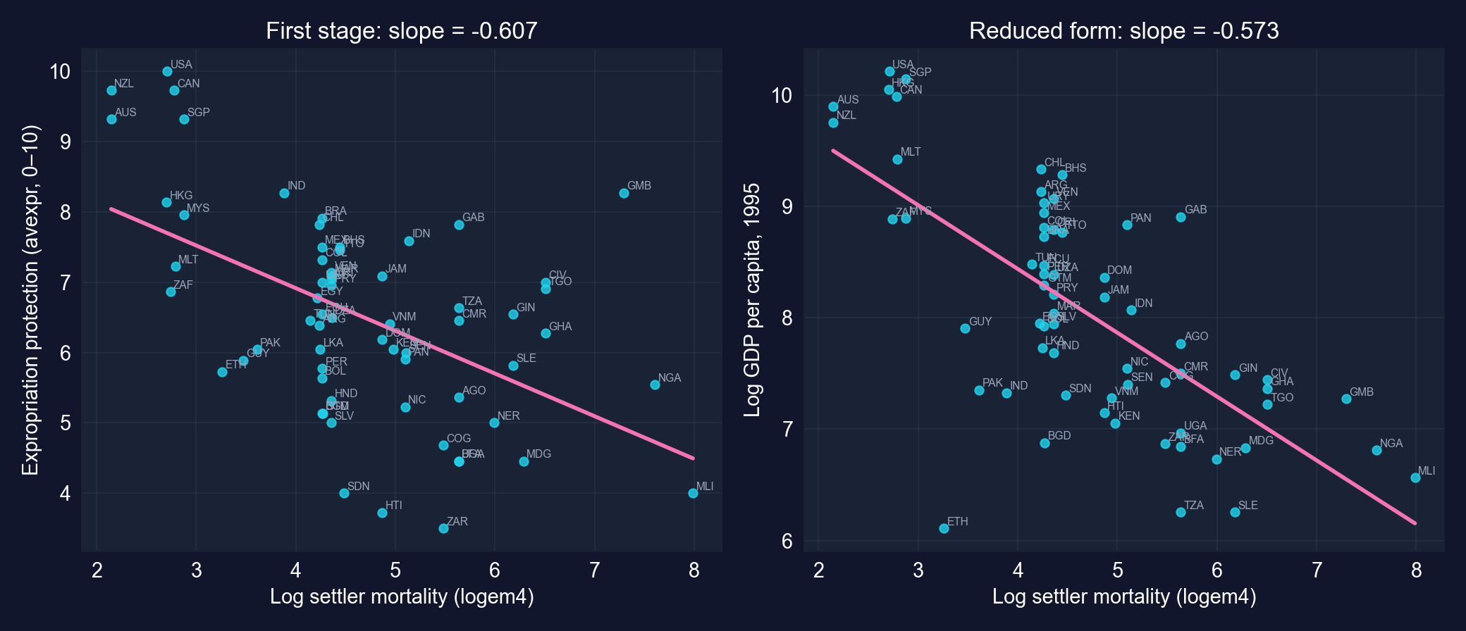
Places deadlier for settlers have weaker property-rights protection today. The instrument is relevant and passes the \(F > 10\) rule of thumb.

A one-unit increase in log settler mortality (mortality about 2.7 times higher) goes with 0.61 points less expropriation protection. The right panel (reduced form) is used two slides ahead.

Code: two-stage least squares in one line

# continues from the previous block
# formula syntax: outcome ~ exogenous regressors | endogenous ~ instrument
fit_iv = pf.feols("logpgp95 ~ 1 | avexpr ~ logem4", data=data_inst, vcov="HC1")  # 2SLS
fit_iv.summary()                            # causal slope under the IV assumptions
print(fit_ols.coef()["avexpr"], fit_iv.coef()["avexpr"])   # OLS vs IV
import numpy as np                          # for np.exp
print(np.exp(fit_iv.coef()["avexpr"]))      # multiplicative effect on GDP: e^b

↗ Try it in Colab

The | separates the exogenous part (1, just the intercept) from the endogenous regressor and its instrument.

pyfixest runs both stages internally and, importantly, computes correct 2SLS standard errors. Running the two stages by hand with OLS gives the right coefficient but wrong SEs.

Output: the IV estimate is 1.8× the OLS estimate

Variable	Coef.	HC1 SE	\(t\)	\(p\)	95% CI
Intercept	1.910	1.193	1.60	0.114	[−0.47, 4.29]
avexpr (instrumented)	0.944	0.179	5.28	< 0.001	[0.587, 1.302]

N = 64 · 2SLS, instrument logem4 · HC1 SEs

One more point of institutional quality causes 0.94 log points higher GDP per capita, if the instrument is valid.

IV coefficient 0.944 vs OLS 0.522 (ratio 1.81, so IV is about 80% larger). Note the SE is 3.6× larger than OLS (0.179 vs 0.050): IV uses only the part of the variation in institutions driven by settler mortality, so it is less precise.

IV = reduced form ÷ first stage

\[\hat\beta_{IV} = \frac{\text{effect of } Z \text{ on } Y}{\text{effect of } Z \text{ on } X} = \frac{-0.573}{-0.607} = 0.944\]

Reduced form: \(-0.573\) is the slope of log GDP on log settler mortality (bivariate OLS, same 64 countries).

IV rescales the instrument’s total effect on GDP by its effect on institutions. All the identifying power comes from settler mortality.

With one instrument and no other regressors, 2SLS equals the ratio of the reduced-form slope to the first-stage slope (indirect least squares). The reduced-form regression (logpgp95 on logem4) is computed for the slides; the ratio reproduces the chapter’s 0.944 exactly. If the exclusion restriction fails, so that mortality affects GDP through some other channel, the numerator includes that channel and the IV estimate is biased.

OLS vs IV: same question, different source of variation

	OLS	2SLS (IV)
Coefficient on avexpr	0.522	0.944
Standard error (HC1)	0.050	0.179
95% CI	[0.42, 0.62]	[0.59, 1.30]
GDP effect of +1 index point, \(100(e^{b}-1)\)	+69%	+157%
GDP effect of +1 SD of avexpr (1.47 points)	×2.2	×4.0
Variation used	all variation in institutions	only the part driven by settler mortality

The IV estimate is larger and less precise. Under the IV assumptions, OLS understated the effect of institutions.

Exact conversions: e^0.944 = 2.57, so +157% (the chapter’s “2.57×”); e^0.522 = 1.69, so +69%. One-SD calculations: 0.944 × 1.47 = 1.39 log points → e^1.39 ≈ 4.0; 0.522 × 1.47 = 0.77 → ≈ 2.2. The “≈ 0.94%” style reading would be wrong: the outcome is in logs and the regressor in index points.

Why is IV larger than OLS?

• The chapter’s explanation, attenuation: measurement error in avexpr biases OLS toward zero; IV, using a variable unrelated to that error, corrects it
• Reverse causation and omitted variables would push OLS up, so a larger IV estimate is consistent with measurement error dominating
• But other readings fit too: with heterogeneous effects, IV estimates a local effect for countries whose institutions were shaped by settler mortality, which need not equal the average effect
• And if the exclusion restriction fails (e.g. the disease environment affects GDP directly), the IV estimate itself is biased

OLS < IV is consistent with attenuation bias. It does not prove it.

The chapter says IV > OLS points to measurement error as the dominant bias. That is a reasonable reading, and AJR (2001) make the same argument, but it is one of several explanations, and students should hold it with appropriate uncertainty.

Threats: everything rests on the exclusion restriction

• Exclusion: settler mortality reflects the disease environment and geography, which may affect GDP directly, not only through institutions
• Other channels: settlers brought human capital, language and legal origin, not just institutions
• Data critique: the settler-mortality series has been challenged (e.g. Albouy 2012), and re-estimates with revised data are weaker
• Weak-instrument margin: \(F = 16.3\) passes the \(F > 10\) rule, but recent work argues standard \(t\)-tests need a much stronger first stage
• Small sample: 64 countries, so a few influential observations matter

IV is only as good as its story. Settler mortality is a famous and influential instrument, and a heavily debated one.

Standard IV caveats and the main published debate: Glaeser et al. (2004) argue settlers brought human capital; Albouy (2012, AER) questions the mortality data. Lee, McCrary, Moreira and Porter (2022, AER) show that valid 5% t-tests need first-stage F above about 104 under the conventional critical value. The chapter’s own caveat: results apply to former colonies, and institutional change is slow.

Case 13.9 · From raw data to final data

Reading · merging · cleaning · the work behind every regression

Case 13.9 is not an estimation case: it is the workflow underneath all the others. Short section: why it matters, then the chapter’s two worked examples (merge, clean).

Most of an empirical project happens before the first regression

Common challenges

• Missing values: drop, impute, or model?
• Outliers: real extremes or typos?
• Units: currencies, inflation, scales
• Frequencies: monthly vs quarterly
• Coding: "M", "m", "Male"

Best practices

• Never overwrite raw data
• Script every step (no manual spreadsheet edits)
• Validate: summary stats before and after
• Report how many rows were dropped and why
• Document every decision

Data preparation often takes 60–80% of a project’s time, and every choice can move the final coefficient.

The chapter’s figure of 60–80% of time on data preparation is a common rule of thumb. The point for students: wrangling choices are modeling choices and must be reported.

Every case in this chapter wrangled its data first

Case	Wrangling step	Why it matters
13.2 Cobb–Douglas	np.log() of \(Q\), \(K\), \(L\); a time index	logs make it linear; HAC needs time order
13.3 Phillips	split at 1970; dropna(subset=["inflgdp1yr"])	the long and short models must share a sample
13.4 Autos	pre-computed logs (lmpg, lcurbwt, …)	elasticities without manual transforms
13.5 RAND	keep year == 1	one observation per person
13.7 Incumbency	drop missing vote (1,390 → 1,297)	no outcome, no observation

Each line changed the estimation sample or the meaning of a coefficient, which is why it belongs in the write-up.

Pulls together the small data steps from the earlier cases. In 13.3, for example, the exact OVB decomposition only holds because the short and long regressions use the same 45 years.

Code: reading formats and merging tables

import pandas as pd                         # tabular data
# data = pd.read_stata("file.dta")          # Stata files
# data = pd.read_csv("file.csv")            # comma-separated text
# data = pd.read_excel("file.xlsx")         # Excel workbooks
df1 = pd.DataFrame({"id": [1, 2, 3], "value_a": [10, 20, 30]})     # table A
df2 = pd.DataFrame({"id": [1, 2, 4], "value_b": [100, 200, 400]})  # table B
print(df1); print(df2)                      # ids 3 and 4 appear in only one table
merged = pd.merge(df1, df2, on="id", how="inner")   # keep ids present in BOTH
print(merged)                               # the inner join result

↗ Try it in Colab

The reading lines are commented out in the chapter (they are templates, not real files). Merge types: how=“inner” keeps matches only; “left” keeps all of df1; “outer” keeps everything, filling gaps with NaN.

Output: an inner join silently drops non-matching rows

id	value_a
1	10
2	20
3	30

df1

id	value_b
1	100
2	200
4	400

df2

id	value_a	value_b
1	10	100
2	20	200

merged (inner join): ids 3 and 4 are gone

Always count rows before and after a merge. Lost observations are lost evidence, and can be a source of selection.

Three rows in, three rows in, two rows out. If the rows that fail to match are systematically different (e.g. small firms missing from one source), the merge itself changes the population you analyze.

Code: cleaning impossible values, gaps and inconsistent codes

import numpy as np                          # np.nan marks missing values
import pandas as pd                         # tabular data
df_dirty = pd.DataFrame({"age": [25, 30, -5, 200, 35],             # two impossible ages
                         "income": [50000, 60000, None, 75000, 80000],  # one missing
                         "gender": ["M", "F", "m", "Female", "M"]})     # inconsistent codes
df_clean = df_dirty.copy()                  # never overwrite the raw data
df_clean.loc[df_clean["age"] < 0, "age"] = np.nan     # impossible: negative age → missing
df_clean.loc[df_clean["age"] > 120, "age"] = np.nan   # impossible: age above 120 → missing
df_clean["income"] = df_clean["income"].fillna(df_clean["income"].median())  # median impute
df_clean["gender"] = df_clean["gender"].str.upper().str[0]   # "m"/"Female" → "M"/"F"
print(df_dirty); print(df_clean)            # before and after

↗ Try it in Colab

The chapter’s cleaning example: detect impossible values, impute a missing value, standardize a categorical variable. Each step is scripted and reversible because the raw frame is kept.

Output: before and after cleaning

age	income	gender
25	50,000	M
30	60,000	F
−5	NaN	m
200	75,000	Female
35	80,000	M

raw

age	income	gender
25	50,000	M
30	60,000	F
NaN	67,500	M
NaN	75,000	F
35	80,000	M

cleaned

Imputation fills the gap with 67,500 (the median of the four observed incomes), but it invents certainty. Flag imputed values and report how many there are.

Median of 50,000, 60,000, 75,000, 80,000 = 67,500. Median imputation shrinks the variance of income and can bias relationships with other variables; a missing-value indicator, or multiple imputation, is more honest. Setting impossible ages to NaN (instead of guessing) is the conservative choice.

Reading it right

Act III · The resolution

Synthesis: compare the four designs, decide which fits a question, revisit the naive-vs-design numbers, and leave with a checklist for interpreting any coefficient.

Four designs, side by side

	RCT (13.5)	DiD (13.6)	RD (13.7)	IV (13.8)
Source of variation	random assignment	group × period	a sharp cutoff	an instrument
Identifying assumption	intact randomization	parallel trends	continuity at the cutoff	relevance + exclusion
Estimand	average effect in the experiment	effect on the treated (ATT)	effect at the cutoff (local)	local average effect (LATE)
Main threat	attrition, non-compliance	pre-trends, other shocks	sorting, functional form	invalid exclusion, weak IV
Testable?	covariate balance	pre-trends (more periods)	density, balance at 0	relevance only (\(F\))
Chapter estimate	−$1,108 (95% plan)	+0.52 z-units	+4.8 pp	0.94 log points

Every design buys credibility with an assumption. Know which assumption you bought, and for whom the estimate holds.

The estimand row matters as much as the estimate: each design answers a slightly different question. RD is local to close races; IV is local to the instrument-driven variation; DiD is for the treated group; the RCT is for experiment participants.

Which design fits your question?

• Can you randomize the treatment? Run an RCT
• Does treatment switch on at a known threshold of a score, margin or date? Use RD
• Do you observe treated and untreated groups before and after treatment? Use DiD, and defend parallel trends
• Is there a variable that shifts the treatment but affects the outcome only through it? Use IV, and defend exclusion
• None of these? Then a regression with controls gives a conditional association; use the OVB formula to sign the likely bias

Start from the source of variation, not from the estimator. The estimator is almost always OLS or 2SLS.

A decision guide, not a strict algorithm: many real studies combine designs (e.g. DiD with an RD-style cutoff, or IV inside an RCT with imperfect compliance).

Naive vs design: how far apart the numbers were

Case	Naive comparison	Naive	Design	Design-based
13.3	bivariate slope, 1970–2014	+0.265	add expected inflation	−0.128
13.6	treated, before vs after	+0.867	DiD	+0.522
13.6	treated vs control, 1998 only	+0.391	DiD	+0.522
13.7	all winners vs all losers	+21.7 pp	RD at the cutoff	+4.8 pp
13.8	OLS	0.522	2SLS	0.944

The naive numbers were not slightly off: the wrong sign (13.3), 66% too large or 25% too small (13.6), 4.5× too large (13.7), 45% below the IV estimate (13.8).

13.3 is not a causal design but an omitted-variable diagnosis; it is included because it shows the same pattern. The RCT has no naive counterpart in the data (everyone was randomized), which is exactly the point: randomization removes the need for one. The bias goes in both directions across cases, so no “rule” says naive estimates are too large.

The tempting mistake — and the correction

Objection. “Just add enough controls and any regression becomes causal.”

Response. Controls close only the confounders you can measure. In 13.1, five controls left the parent-education slope almost unchanged, and that is no evidence it is causal. In 13.7, comparing winners with losers gives 21.7 points; the cutoff gives 4.8.

Identification comes from the design, not the dataset. Ask “where does the variation come from?” before asking “what is the coefficient?”

Steelman the objection: controls do help, and the OVB formula shows how. But stability of a coefficient when controls are added is not proof of causality, because the variables that matter most are often the ones you do not observe.

Five questions to ask of any coefficient

1. Units: levels, logs or both? An elasticity, a semi-elasticity (\(100(e^b-1)\%\)), percentage points, or \(z\)-units?
2. Conditional on what? Which variables are held fixed, and which are not?
3. Which standard error? HC1, HAC or clustered: does it match how the data were generated?
4. Where does the variation come from? Self-selection, randomization, a trend break, a cutoff, an instrument?
5. For whom? Everyone (ATE), the treated (ATT), close races (local), or instrument-compliers (LATE)?

The most common misreadings come from skipping question 1: “4.8%” instead of 4.8 percentage points, “0.52 SD” without saying which SD, or “1%” for a percentage-point change.

A checklist students can apply to any regression output. The unit errors corrected in this deck: RD effect in percentage points (not %), DiD effect in reference-population z-units (not sample SDs), Phillips slope in percentage points of inflation per percentage point of unemployment, and log-outcome effects converted with e^b − 1.

What to carry forward

• One estimator, nine questions: pf.feols from school scores to the wealth of nations
• Logs give elasticities; the sum of Cobb–Douglas elasticities tests returns to scale
• An omitted variable can flip a sign, and \(E[b_2]=\beta_2+\beta_3\gamma\) says exactly by how much
• Match the standard error to the data: HC1, NW for time series, CRV1 for groups; in 13.4 clustering changed SEs 6–9×
• RCT / DiD / RD / IV each impute the counterfactual differently, and each rests on an assumption you must defend
• Wrangling is modeling: every sample restriction belongs in the write-up

Recap of the chapter’s Key Takeaways, updated with what the deck verified: exact OVB decomposition, the size of the clustering correction, the naive-vs-design gaps, and the unit conventions.

Nine case files, one lesson: a causal slope is earned by design, not by adding controls.