Categories in a regression
Act I · The tension
Not every regressor is a number
Education and age slot straight into a regression — they’re continuous. But gender, sector, region are categories. How do you put “female” or “government worker” into an equation that multiplies coefficients by numbers?
The trick is the indicator variable: code the category as \(0\) or \(1\). Then a single regression measures group gaps, tests them, and even lets each group have its own slope.
Where we’re going
- An indicator (\(0/1\)) shifts the intercept between two groups
- Regression on one dummy is a difference-in-means test
- Add controls → the conditional gap; add an interaction → different slopes
- Separate regressions + the Chow test → do groups share one model?
- Sets of dummies → the dummy-variable trap, base categories, and ANOVA
Six ideas anchor this chapter
- Indicator (dummy) — \(1\) in a category, \(0\) otherwise; shifts the intercept
- Base category — the omitted group the intercept represents; others are measured against it
- Slope dummy — an interaction \(d\times x\) that lets the slope differ by group
- Conditional vs unconditional gap — the raw mean difference vs the gap after controls
- Chow test — an \(F\)-test of pooled-vs-separate regressions
- Dummy-variable trap — all categories + intercept = perfect collinearity
A dummy moves the intercept; an interaction moves the slope; an \(F\)-test tells you if either moved for real.
From a gap to a model
Act II · The investigation
14.1 — A single indicator is a difference in means
!pip install -q pyfixest                     # pyfixest not preinstalled in Colab
import pandas as pd                          # tabular data
import pyfixest as pf                         # OLS with R-style formulas

url  = "https://raw.githubusercontent.com/quarcs-lab/data-open/master/AED/AED_EARNINGS_COMPLETE.DTA"
data = pd.read_stata(url)                    # 872 full-time workers (gender: 1=F, 0=M)

fit = pf.feols("earnings ~ gender", data=data, vcov="HC1")   # HC1 robust SEs
fit.summary()
# Intercept ≈ 63,000 = MALE mean · gender coef ≈ −16,396 = female−male gap (robust t ≈ −5.1)With one dummy, the intercept is the base-group mean and the slope is the gap — regression is a two-sample t-test. The raw gap: women earn ~$16k less.
14.2 — Controls give the conditional gap (and it can widen)
# genderbyeduc = gender × education  (a precomputed interaction column)
m2 = pf.feols("earnings ~ gender + education", data=data, vcov="HC1")

m3 = pf.feols("earnings ~ gender + education + genderbyeduc",   # + slope dummy
              data=data, vcov="HC1")
print(m2.coef()["gender"])                   # ≈ −18,258  (gap WIDENS vs −16,396!)
print(m3.coef()["genderbyeduc"]) # return to schooling differs by genderControlling for education widens the gap to ~$18k: women here are more-educated on average, so holding education fixed exposes more of the unexplained gap. Controls can move a coefficient either way.
14.3 — An interaction lets each group keep its own slope
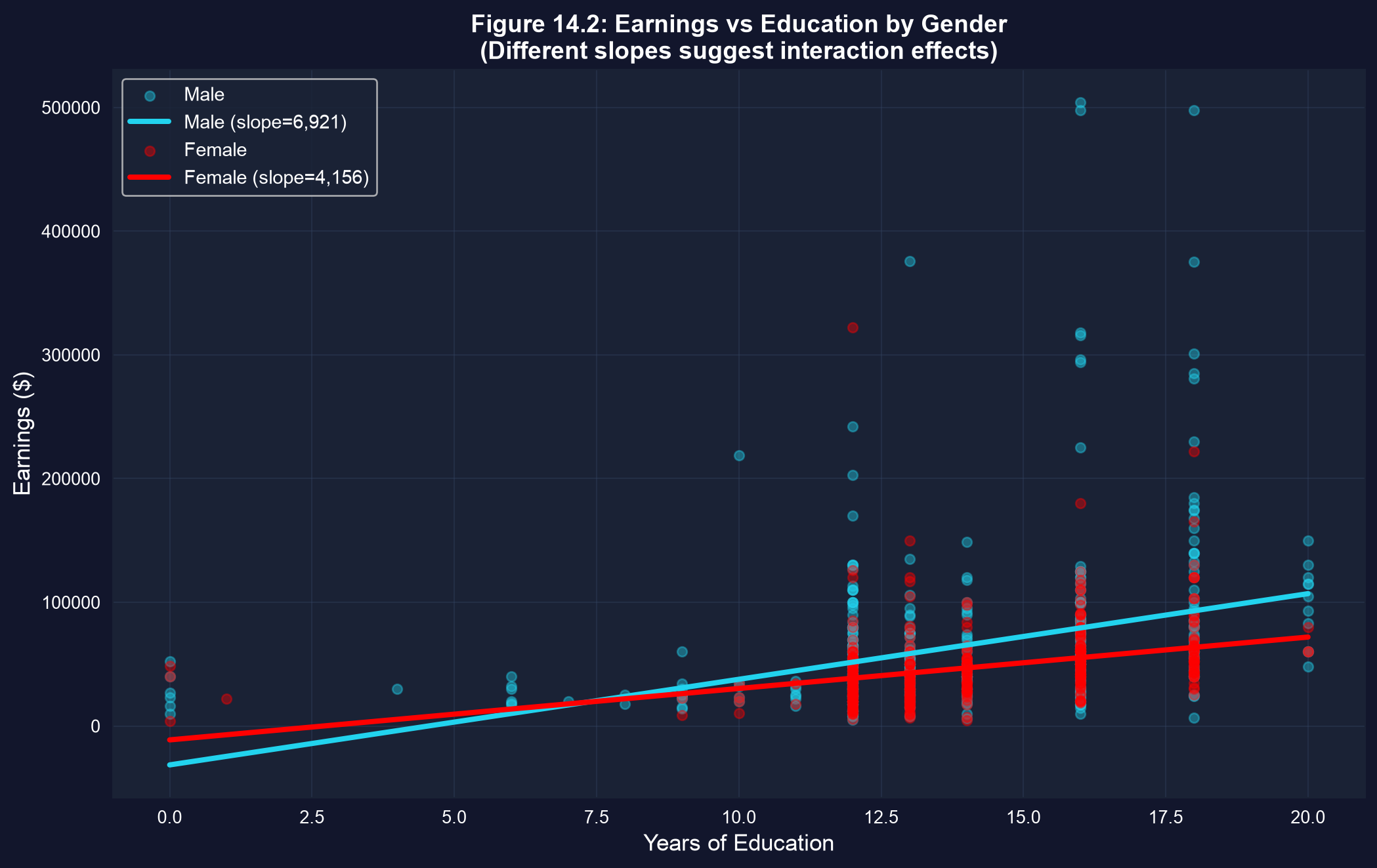
Earnings vs. education, fit separately by gender. The lines aren’t parallel — men’s return to a year of schooling (~$6,300) is steeper than women’s (~$4,200).
Non-parallel lines are the interaction: \(\hat y = (b_1+a_1) + (b_2+a_2)x\) for women vs \(b_1+b_2x\) for men. The slope dummy \(a_2\) is the difference in returns.
14.4 — Separate regressions + a Chow test
# Fit the SAME model on each subsample — every coefficient free to differ
f = pf.feols("earnings ~ education + age + hours", data=data.query("gender==1"))
m = pf.feols("earnings ~ education + age + hours", data=data.query("gender==0"))

print(f.coef()["education"], m.coef()["education"])   # ≈ 4,200 (F) vs 6,300 (M)
print(f.coef()["hours"],     m.coef()["hours"])       # ≈   700 (F) vs 1,600 (M)
# Chow test of H0: β_F = β_M = robust joint test on all 4 gender terms of the fully
# interacted model: Wald χ² ≈ 32.6 (4 restr.), F ≈ 8.1, p < 0.001 → REJECTS poolingDifferent slopes on education and hours — not just a constant gap. The Chow test formalizes “do men and women need different equations?” Its robust version, the joint test on all four gender terms of the fully interacted model (\(F\approx8.1\), \(p<0.001\)), says yes.
14.5 — Many categories: mind the dummy-variable trap
# Worker type: dself, dprivate, dgovt — these sum to 1 for every worker,
# so all three PLUS an intercept = perfect collinearity (the "trap").
fit = pf.feols("earnings ~ dself + dgovt + education + age",   # drop dprivate = base
               data=data, vcov="HC1")
fit.summary()
# dself ≈ +17,000 · dgovt ≈ −2,000 → gaps vs the PRIVATE-sector baseDrop one category (or the intercept). The base is the intercept’s group; every coefficient is a gap from the base. Changing the base re-labels gaps but leaves \(R^2\approx0.12\) untouched.
A set of indicators with no controls is ANOVA
data["typeworker"] = (1*data.dself + 2*data.dprivate + 3*data.dgovt).astype(int)

fit = pf.feols("earnings ~ C(typeworker)", data=data)   # C() = treat as categorical

# the regression's joint F-test equals the one-way ANOVA F-statistic:
from scipy.stats import f_oneway                          # scipy (preinstalled)
print(f_oneway(*[g.earnings for _, g in data.groupby("typeworker")]))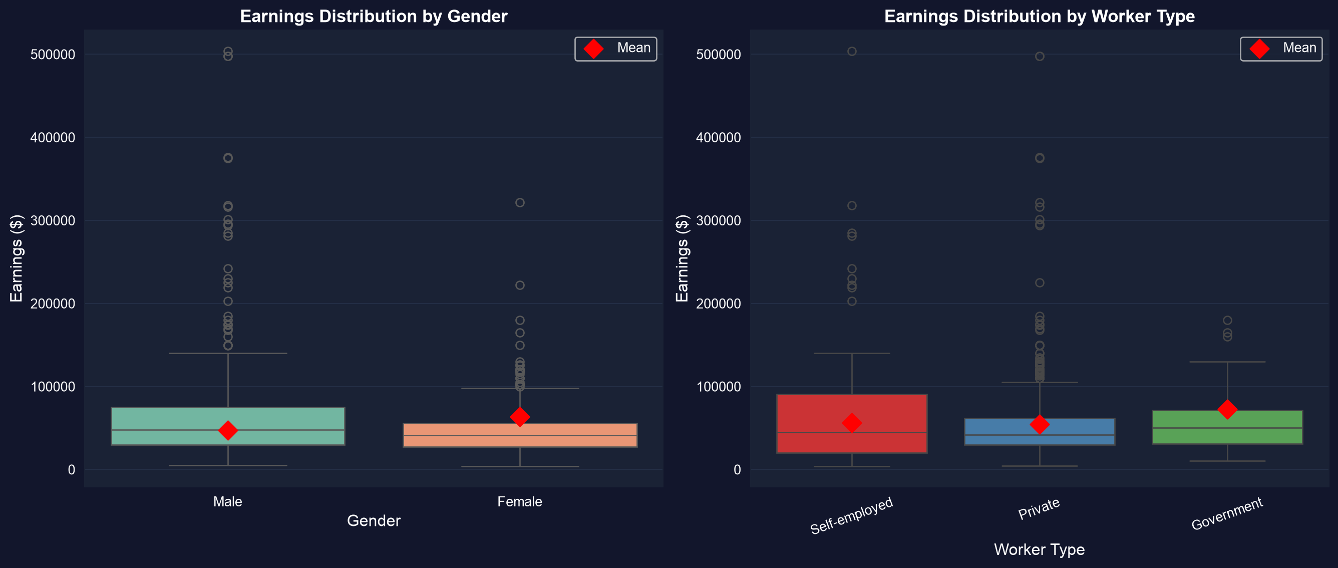
Earnings by gender (left) and worker type (right) — the group means the indicators recover.
Reading it right
Act III · The resolution
Two traps when a category enters more than once
Objection. “The gender×education term isn’t significant on its own, so gender’s effect through education is zero.”
Response. When a category enters as a level + interactions, the terms are correlated — individual \(t\)-tests mislead. Use a joint \(F\)-test on all gender terms (here Wald \(\chi^2\approx32.6\) with 4 restrictions, i.e. \(F\approx8.1\), \(p<0.001\)). And remember the gap is descriptive, not proof of discrimination.
Test categorical effects jointly; interpret gaps as associations until a design earns the causal reading.
What to carry forward
- Code a category as a \(0/1\) indicator; its coefficient is a group gap, and one dummy = a difference-in-means test.
- Adding controls gives the conditional gap — which can shrink or widen (suppression).
- An interaction \(d\times x\) is a slope dummy — non-parallel group lines; separate regressions + the Chow test check the whole model.
- For \(C\) categories keep the intercept and drop one dummy (base category) to avoid the trap; the choice changes labels, not fit.
- Indicators-only regression = ANOVA, with the same joint \(F\)-test.