The problem

Act I · Straight lines don’t fit everything

Real economic relationships bend

Earnings don’t rise with age in a straight line — they climb fast when you’re young, flatten in mid-career, and fall near retirement. A plain earnings ~ age line misses all of it.

The fix isn’t to abandon OLS. It’s to transform the variables — logs, squares, interactions — so a model that is still linear in its coefficients can trace a curved story.

The whole chapter rests on one idea: “linear regression” means linear in the parameters, not in the variables. Once you accept that, logs and polynomials open up without leaving the OLS toolkit.

Where we’re going

• Logs — level-log, log-linear, log-log, and the percentage/elasticity each implies
• Quadratics — capture the inverted-U life-cycle of earnings
• Standardized coefficients — compare regressors measured in different units
• Interactions — let the return to education change with age
• Marginal effects — AME, MEM, MER — when the slope itself varies
• Prediction — undo a log transform without retransformation bias

Five ideas anchor this chapter

• Marginal effect — the change in \(y\) per one-unit change in \(x\); once \(x\) enters nonlinearly, it varies with \(x\)
• AME · MEM · MER — average the effect, evaluate it at the mean, or at chosen profiles
• Polynomial regression — add \(x^2\) (then \(x^3\)…) to bend the line, still linear in \(\beta\)
• Standardized coefficient — effect of a 1-SD change in \(x\) on \(y\), in SD units — a common currency
• Smearing estimator — Duan’s residual-based fix for the bias in \(\exp(\widehat{\ln y})\)

One dataset — 872 workers — runs through every transformation.

Our data: 872 workers, earnings and its drivers

AED_EARNINGS_COMPLETE.DTA — 872 full-time workers aged 25–65 (2000), with earnings, age, education, hours, sector, and gender.

import pandas as pd                          # tabular data
import numpy as np                           # logs, squares, z-scores

url = "https://raw.githubusercontent.com/quarcs-lab/data-open/master/AED/AED_EARNINGS_COMPLETE.DTA"
data = pd.read_stata(url)                    # 872 full-time workers, aged 25-65, year 2000

data[["earnings", "age", "education"]].describe().round(1)   # scale before you model

↗ Try it in Colab

pandas/numpy are preinstalled in Colab, so no pip install here. Mean earnings ≈ $56k; the log models below tame that right-skew.

Four ways to bend the line

Act II · The transformations

Logs change what the coefficient means

Three specifications of the same relationship — and three different interpretations.

import pyfixest as pf                                 # OLS with R-style formulas
# (pandas, numpy already loaded; data = AED_EARNINGS_COMPLETE)
data["lnage"] = np.log(data["age"])                   # log of age, for the log-log model
# lnearnings already in the data; = np.log(earnings)

levels  = pf.feols("earnings   ~ age   + education", data=data, vcov="HC1")  # $ per unit
loglin  = pf.feols("lnearnings ~ age   + education", data=data, vcov="HC1")  # % per unit (Mincer)
loglog  = pf.feols("lnearnings ~ lnage + education", data=data, vcov="HC1")  # elasticity on age

loglin.summary()                                      # the Mincer earnings equation

↗ Try it in Colab

HC1 = heteroskedasticity-robust SEs, the chapter’s default. pyfixest is NOT preinstalled in Colab, so the full self-contained version adds !pip install -q pyfixest at the top (see the next tool-heavy slide).

The same data, three interpretations of “age”

• Levels — \(\hat\beta_{\text{age}} \approx \$525\): each extra year adds about $525, no matter the starting earnings.
• Log-linear (Mincer) — \(\hat\beta_{\text{age}} \approx 0.008\): each year is about +0.8% — a semi-elasticity; the dollar amount scales with earnings.
• Log-log — \(\hat\beta_{\ln\text{age}} \approx 0.35\): a 1% rise in age → ≈0.35% rise in earnings — an elasticity (< 1, inelastic).
• Education is the star: ≈ 0.10 in the log models — the famous ~10%-per-year Mincer return.

Log-linear \(\beta\) as a percent is an approximation — the exact effect is \(100(e^{\beta}-1)\%\), and the gap matters once \(|\beta| > 0.1\).

A quadratic captures the life-cycle hump

Add age-squared: the slope on age is now \(\beta_2 + 2\beta_3\,\text{age}\) — it changes with age.

!pip install -q pyfixest                     # pyfixest isn't preinstalled in Colab (-q = quiet)
import pandas as pd; import numpy as np; import pyfixest as pf
url = "https://raw.githubusercontent.com/quarcs-lab/data-open/master/AED/AED_EARNINGS_COMPLETE.DTA"
data = pd.read_stata(url)                     # 872 workers

quad = pf.feols("earnings ~ age + I(age**2) + education", data=data, vcov="HC1")  # age + age^2
b2, b3 = quad.coef()["age"], quad.coef()["I(age ** 2)"]    # linear & quadratic terms

turning_point = -b2 / (2 * b3)                # age where the slope hits zero (earnings peak)
print(f"peak earnings at age {turning_point:.0f}")         # ~ 52
print(f"marginal effect at 25: {b2 + 2*b3*25:,.0f}")       # ~ +$1,600 / yr
print(f"marginal effect at 60: {b2 + 2*b3*60:,.0f}")       # ~ -$450 / yr

↗ Try it in Colab

Linear age coef ≈ +$3,000–5,000, agesq ≈ −$30 to −$50. The joint F-test on age and age² is highly significant, so the curvature is real, not noise.

Earnings peak near age 52, then decline

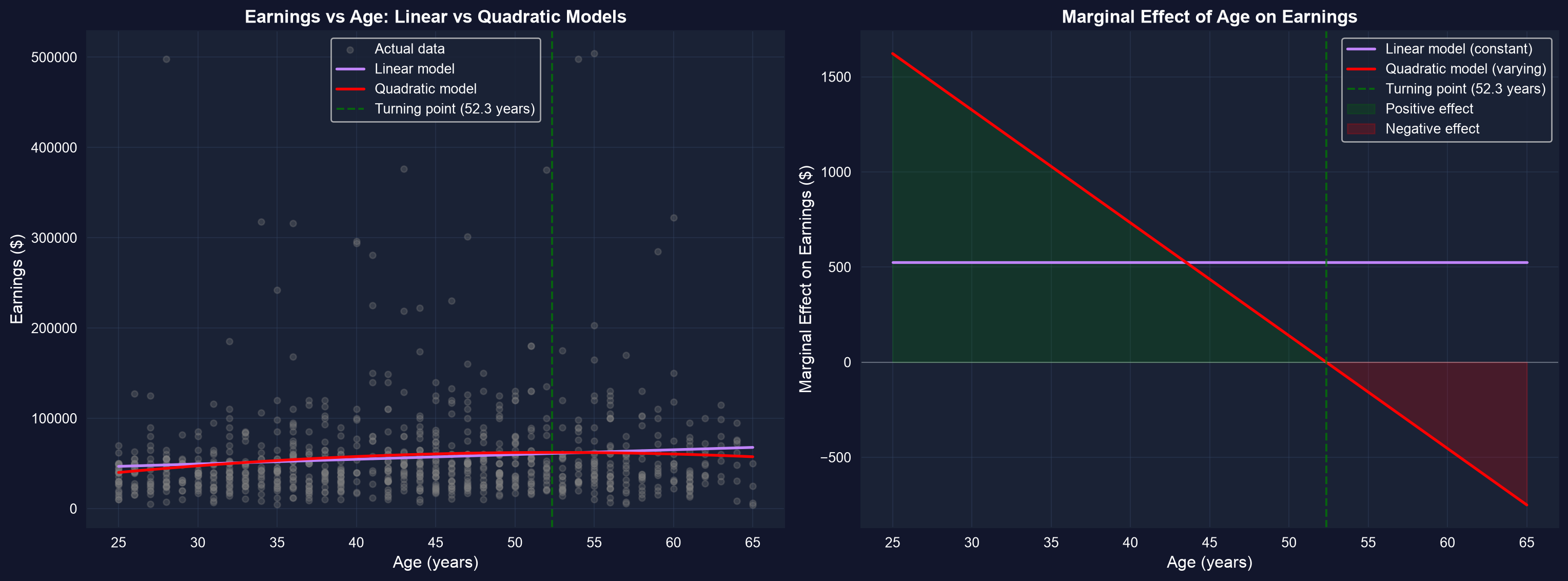
Fitted earnings against age (education held at its mean): the inverted-U life-cycle profile the quadratic recovers.

The slope is +$1,600/yr at 25, $0 near age 52, and −$450/yr at 60 — one regressor, three marginal stories.

Standardize to compare apples and oranges

Dollars-per-year and log-hours can’t be compared raw. Re-express every variable in SD units.

# z-score each variable: (x - mean) / sd  → coefficients become "SD of y per SD of x"
cols = ["earnings", "age", "agesq", "education", "lnhours"]
z = data[cols].apply(lambda s: (s - s.mean()) / s.std())      # standardized copies

mz = pf.feols("earnings ~ age + agesq + education + lnhours", data=z, vcov="HC1")
mz.coef().round(3)      # beta* weights — now directly comparable
# age & age^2 dominate; among the rest, education and lnhours carry the most weight

↗ Try it in Colab

Standardized weights rank the drivers

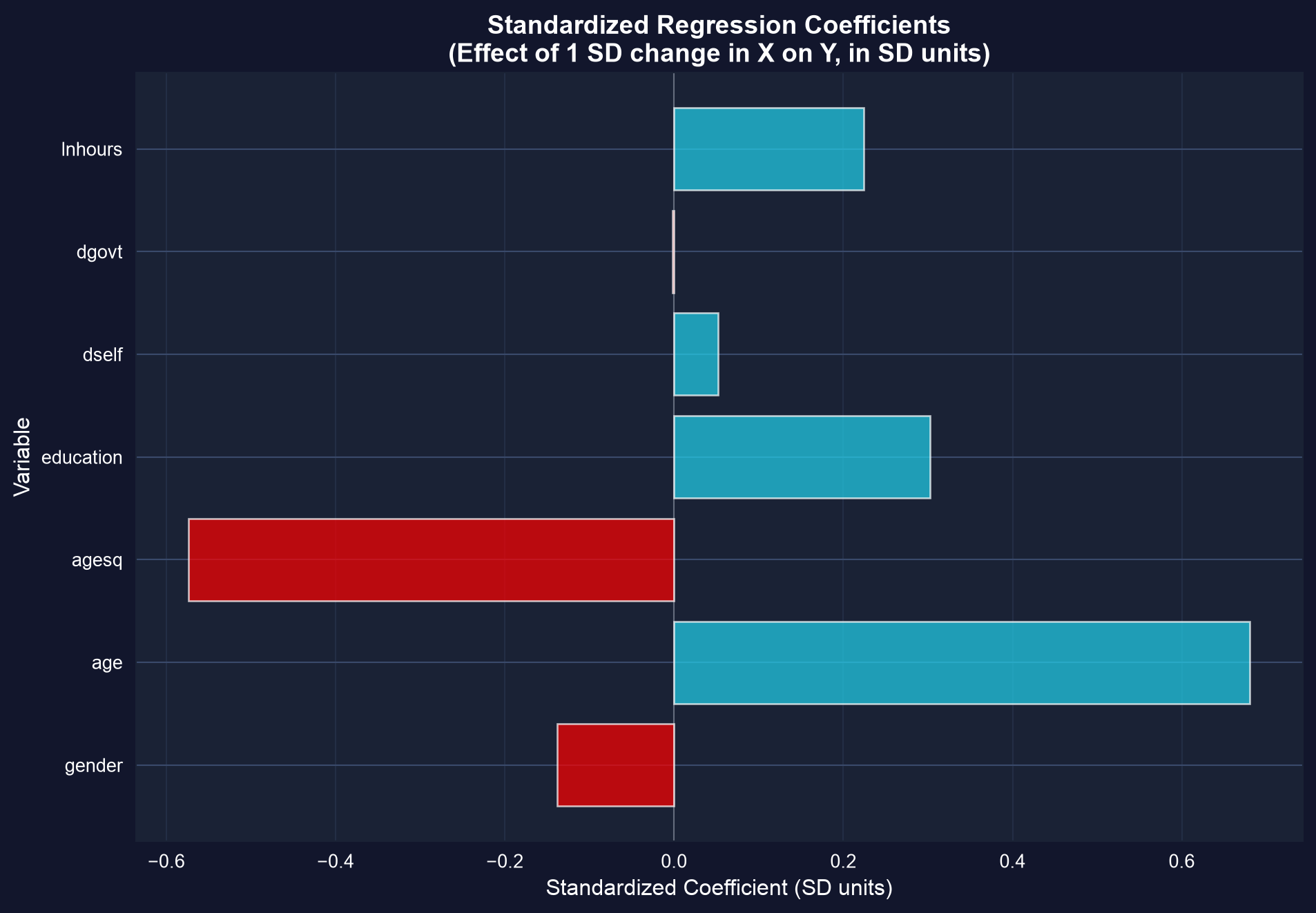
Standardized (\(\beta^*\)) coefficients: age and its square dominate; education and log-hours lead the rest.

A standardized coefficient answers “which regressor moves earnings most per SD of effort?” — comparable across units.

Interactions let the return to education shift with age

Does a year of schooling pay the same at 25 as at 55? Multiply the two regressors and test it.

inter = pf.feols("earnings ~ age * education", data=data, vcov="HC1")   # age, education, age:education

# return to education at a given age = beta_educ + beta_(age:educ) * age
be, bx = inter.coef()["education"], inter.coef()["age:education"]
print(f"return at 25: {be + bx*25:,.0f}")     # ~ +$5,241 / education-year
print(f"return at 55: {be + bx*55:,.0f}")     # ~ +$6,112 / education-year

# is the interaction itself distinguishable from zero?
inter.wald_test(R=[[0, 0, 0, 1]])             # H0: beta_(age:education) = 0  -> p ~ 0.60

↗ Try it in Colab

age * education expands to age + education + age:education. The returns drift from $5,241 at 25 to $6,112 at 55 — only ~1.2×, and the interaction is not significant (p ≈ 0.60), so read it cautiously.

Predicting from a log model: beware retransformation bias

\(\exp(\widehat{\ln y})\) predicts the median, not the mean — it systematically underpredicts. Duan’s smearing correction fixes it with the residuals themselves.

logmod = pf.feols("lnearnings ~ age + education", data=data, vcov="HC1")  # s_e ~ 0.62

naive = np.exp(logmod.predict())                        # biased: ~ $46k mean (actual ~ $56k)

smear = np.exp(logmod.resid()).mean()                   # Duan factor = mean(exp(residuals)) ~ 1.21
corrected = naive * smear                               # smeared prediction
print(f"naive mean     {naive.mean():,.0f}")            # ~ 46,000
print(f"corrected mean {corrected.mean():,.0f}")        # ~ 55,000, matches the data

↗ Try it in Colab

Jensen’s inequality: E[exp(u)] > exp(E[u]). The normality factor exp(s_e²/2) ≈ exp(0.62²/2) ≈ 1.21 gives the same correction when residuals are roughly normal; Duan’s smearing needs no such assumption.

Naive exp() underpredicts; smearing restores the mean

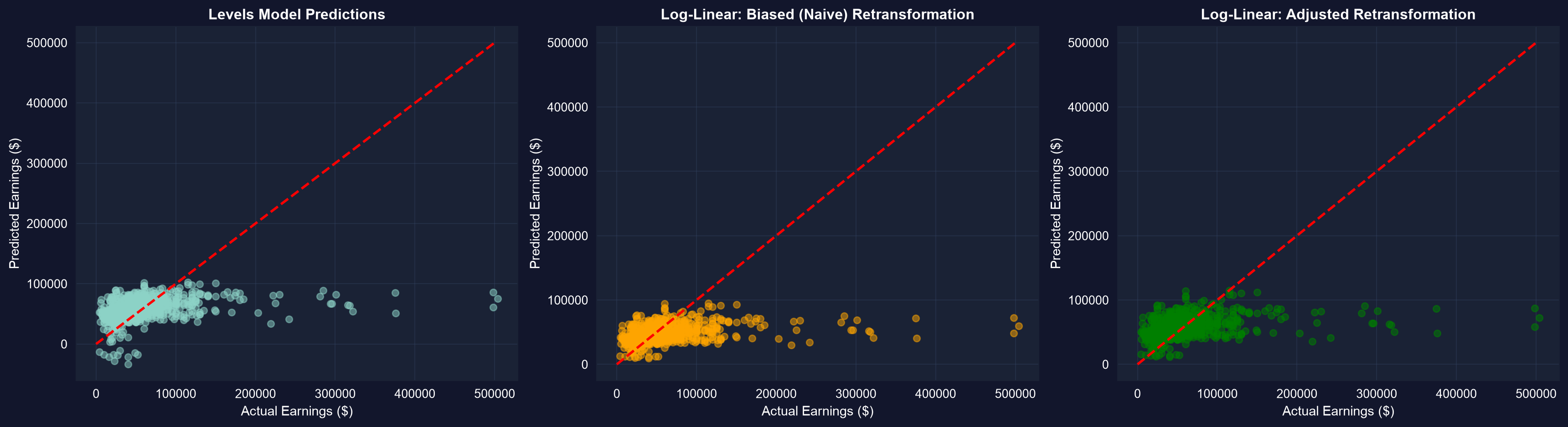
Predicted vs actual earnings: the naive \(\exp(\widehat{\ln y})\) sits low; the smeared prediction lands on the 45° line.

Always smear before you report dollar predictions from a log model.

Reading transformed coefficients right

Act III · The interpretation traps

Three traps, three corrections

Trap. “Log-linear \(\beta = 0.12\) means exactly +12%, and the log-log model fits best because its \(R^2\) is highest.”

Correction. The percent is an approximation (\(100(e^{0.12}-1) \approx 12.7\%\)); and you cannot compare \(R^2\) across models whose dependent variable differs (\(y\) vs \(\ln y\)) — judge them on prediction accuracy or economic plausibility instead.

A transformed coefficient is only as good as its interpretation — know whether you’re reading dollars, percents, or elasticities.

What to carry forward

• Logs give percentages and elasticities; the %-reading is approximate — use \(100(e^{\beta}-1)\) when \(|\beta|\) is large.
• Quadratics make the marginal effect vary; report the turning point and a few representative slopes (MER).
• Standardize to rank regressors across units; interact to let one effect depend on another — then test it.
• Don’t compare \(R^2\) across different dependent variables; smear before predicting levels from a log model.
• Every transformation keeps OLS linear in the coefficients — the toolkit never changed.

Transform the variable, not the method — then read the coefficient for what it truly is.