Act I — The Question

How much should a society save?

Solow handed households a saving rate — what if they chose it?

In the Solow model, households save a fixed fraction of income, whatever happens.

Real households decide: consume today, or save and consume more tomorrow?

Making saving a choice turns a growth model into a model of optimal behaviour — and lets us judge outcomes.

Ramsey (1928), revived by Cass and Koopmans in the 1960s. Without preferences, Solow cannot say whether an outcome is good. The policy question: how much should a society save for its future?

The naive answer — save enough to maximise consumption forever — is wrong

Solow’s golden rule

• pick the capital stock that maximises steady-state consumption
• ignores what it costs to get there

Ramsey’s optimum

• maximise discounted lifetime utility
• counts the sacrifices on the way

Optimal saving weighs the transition, not just the destination.

Set up the comparison we resolve with the modified golden rule.

Where we’re going

• The question: how should households split income between today and tomorrow?
• The model: the Hamiltonian, the Euler equation, the phase diagram, shocks
• So what: what the data say about \(\sigma\) and \(r > g\), Piketty, and the social discount rate

Advanced objectives: read a phase diagram and explain why only the saddle path is an equilibrium; evaluate Piketty’s r > g within the model.

Two kinds of variables: capital is sticky, consumption can jump

Capital \(k\) — the state

• built by past saving
• changes only gradually

Consumption \(c\) — the control

• chosen freely each instant
• can jump when news arrives

When something changes, consumption absorbs the surprise and capital follows.

The state/control distinction drives the saddle-path logic later.

The planner, one household, infinite lives — defensible shortcuts

• Planner: under the welfare theorems it reproduces the competitive outcome
• One household: fine if people respond similarly to incentives
• Infinite lives: dynastic altruism, as in Barro (1974)
• Discounting: positive interest rates reveal impatience

Caselli and Ventura (2000): structured heterogeneity still aggregates to a representative household. We check the planner shortcut at the end of Act II: the decentralised economy gives the same answer.

Act II — The Model

Optimal saving, step by step

Households maximise discounted utility of everyone alive

\[\int_0^\infty u(c_t)\, e^{nt} e^{-\rho t}\, dt \qquad \text{s.t.} \qquad \dot k_t = f(k_t) - n k_t - c_t\]

Population grows at \(n\); the future is discounted at \(\rho > n\); capital grows by output minus consumption minus “capital widening” \(nk\) (no depreciation).

rho greater than n: otherwise the problem has no solution (footnote 5). Book eqs. 3.1 and 3.5.

The Hamiltonian prices capital with a shadow value λ

\[H = u(c)\,e^{nt} + \lambda\,\big[f(k) - nk - c\big]\]

\(\lambda_t\), the co-state, is the value at \(t\) of one more unit of capital: a shadow price, like a Lagrange multiplier.

Static condition: \(u'(c)e^{nt} = \lambda\), so the marginal value of consuming equals the marginal value of saving.

Book eqs. 3.6–3.7. The current-value Hamiltonian. c is the control, k the state.

Capital is an asset: its return must equal its opportunity cost

\[\rho + n = \frac{\dot\lambda}{\lambda} + f'(k)\]

Opportunity cost of holding capital (\(\rho + n\)) = dividend (\(f'(k)\)) + capital gain on its price (\(\dot\lambda/\lambda\)).

The arbitrage logic we reuse for investment, asset prices and policy.

Book eq. 3.10, the dynamic FOC rewritten as an asset-pricing condition.

The Euler equation: consumption grows when saving pays more than impatience costs

\[\frac{\dot c_t}{c_t} = \sigma\,\big[f'(k_t) - \rho\big], \qquad \sigma \equiv -\frac{u'(c)}{u''(c)\,c}\]

Differentiate the static condition in time and use the arbitrage condition. \(\sigma\) is the elasticity of intertemporal substitution.

Every intertemporal choice in the book is a variation on this equation.

Book eqs. 3.13–3.15. Derivation in the guide’s Derivations page and Exercise 6.

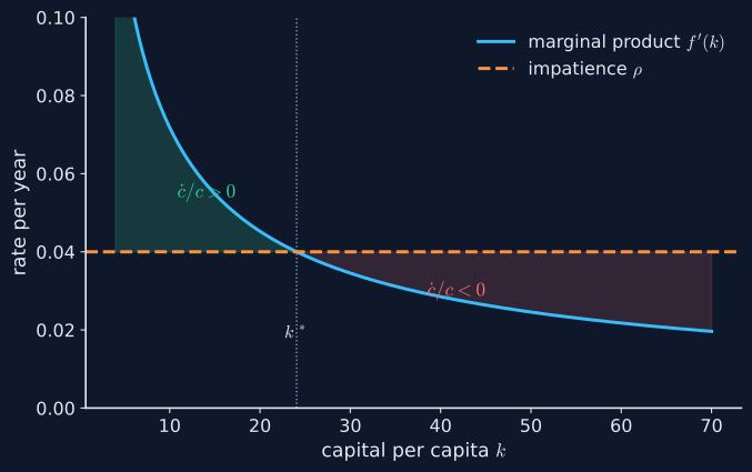
Consumption grows to the left of k*, where capital’s return beats impatience

The Euler equation in one picture (illustrative parameters)

Where the marginal product exceeds rho, consumption grows. sigma does not move the crossing, only the speed.

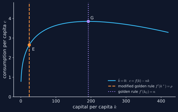
Optimal saving stops short of the golden rule

The kdot = 0 locus peaks at the golden rule; the optimum E lies to its left (illustrative)

Discounting (\(\rho > n\)) makes the consumption-maximising capital stock not worth building.

E has much less capital than G.

The modified golden rule pins the steady state

\[f'(k^*) = \rho \;>\; n = f'(k_G) \quad\Longrightarrow\quad k^* < k_G\]

Optimal saving never oversaves: no dynamic inefficiency, unlike Solow.

Chapter 8 returns to oversaving with overlapping generations.

With illustrative numbers, the optimum holds one eighth of the golden-rule capital

\(f(k) = k^{1/3}\), \(\rho = 0.04\), \(n = 0.01\) (the guide’s worked example):

	Capital \(k\)	Consumption \(c\)
Optimum (modified golden rule)	24.06	2.646
Golden rule	192.45	3.849

\(k^*/k_G = (n/\rho)^{1/\alpha} = 0.125\): discounting matters enormously.

Numbers from the guide’s worked example and Exercise 2, verified by _verify.py.

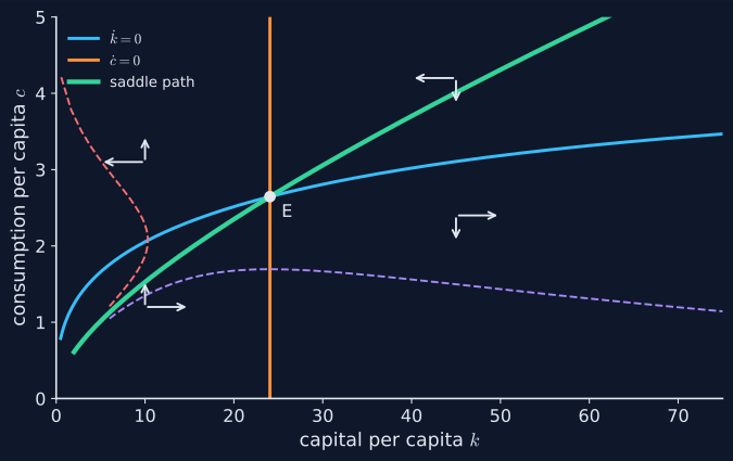
Only the saddle path reaches the steady state

Phase diagram: arrows show the motion in each region; dashed paths diverge (illustrative)

Given \(k_0\), consumption jumps onto the saddle path; then both move along it to E.

Above the hump capital falls; left of cdot = 0 consumption rises. The dashed paths start too high (capital runs out) or too low (capital over-accumulates).

Why every other path fails: the transversality condition

• Too much consumption: capital runs to zero, then consumption collapses: infeasible
• Too little consumption: capital piles up past the golden rule, where \(f'(k) < n\): valuable capital is never consumed
• The transversality condition rules both out and selects the saddle path

Uniqueness needs as many unstable roots as jump variables, here one.

Transversality: never die holding valuable capital. Counting rule: one jump variable (c), one unstable eigenvalue. A sink would mean indeterminacy.

A parameter sweep shows how patience raises steady-state consumption

import numpy as np                         # arrays and maths
import matplotlib.pyplot as plt            # plotting
alpha, n = 2/3, 0.01                       # illustrative parameters
rhos = np.linspace(0.015, 0.08, 100)       # impatience rates, all above n
k_star = ((1 - alpha) / rhos) ** (1 / alpha)   # optimum for each rho
c_star = k_star ** (1 - alpha) - n * k_star    # consumption on kdot = 0
fig, ax = plt.subplots()                   # one panel
ax.plot(rhos, c_star)                      # lower rho → higher c*
ax.set_xlabel("impatience ρ"); ax.set_ylabel("steady-state c*")
plt.show()
print(round(c_star[0], 2), round(c_star[-1], 2))   # patient vs impatient

↗ Run the full model in Colab

As rho falls towards n, c* rises towards the golden-rule maximum. The notebook’s Advanced section does this with full saddle paths and two self-checked tasks.

Comparative statics: what moves, on impact and in the long run

Change	On impact	Long run: \(k^*\), \(c^*\)
\(\rho\) ↓ (permanent)	\(c\) jumps down	both ↑
\(\rho\) ↑ (permanent)	\(c\) jumps up	both ↓
\(\sigma\) ↑	faster adjustment	unchanged
\(n\) ↑	\(c\) jumps down to the new \(c^*\)	\(k^*\) unchanged; \(c^*\) ↓

The steady state depends on \(\rho\), \(n\) and technology, not on \(\sigma\).

From the guide’s cheat sheet. n up: the hump falls; k* is unchanged because f’(k*) = rho.

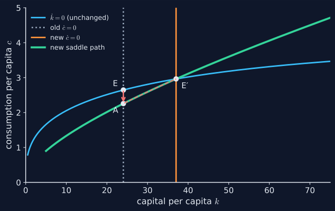
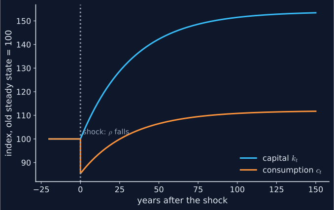
More patience: consumption dips, then climbs to a higher steady state

A permanent fall in ρ: jump from E down to A, then up the new saddle path to E′ (illustrative)

With these numbers consumption falls about 15% on impact, and ends about 12% higher.

rho falls from 0.04 to 0.03 (illustrative). Verified numbers: impact −14.7%, long run +12.0%. New k* ≈ 37.04.

On impact only consumption moves; capital follows gradually

Time paths after the fall in ρ, relative to the old steady state (illustrative)

A higher sigma makes the adjustment faster: half-life about 26.5 years with sigma = 0.5, 11 with sigma = 2 (model notebook).

Act III — So What

What it means for data and policy

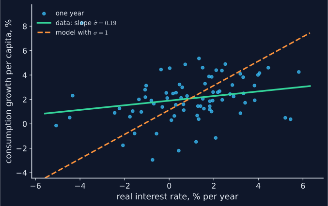
US consumption barely responds to interest rates

Consumption growth vs the real interest rate, US 1948–2025

Source: FRED (BEA, Federal Reserve Board), snapshot 2026-10-15 · the data lab · notebook

Right direction, weak strength: the estimated slope is about 0.19, far below σ = 1.

The lab’s estimate: sigma-hat ≈ 0.19, HAC SE ≈ 0.12, 95% CI includes zero, R² ≈ 5%. Hall (1988) concluded intertemporal substitution is weak.

Why the Euler equation fits poorly in simple data

• Ex-post real rates mismeasure the ex-ante rates savers face
• The T-bill rate is a safe return, not the return on capital \(f'(k)\)
• Some households are liquidity-constrained; habits smooth consumption
• Consumption and interest rates are both endogenous

A small σ means interest rates move consumption only modestly: a lesson for monetary policy.

Caveats from the data lab. Link to monetary policy chapters 19–21.

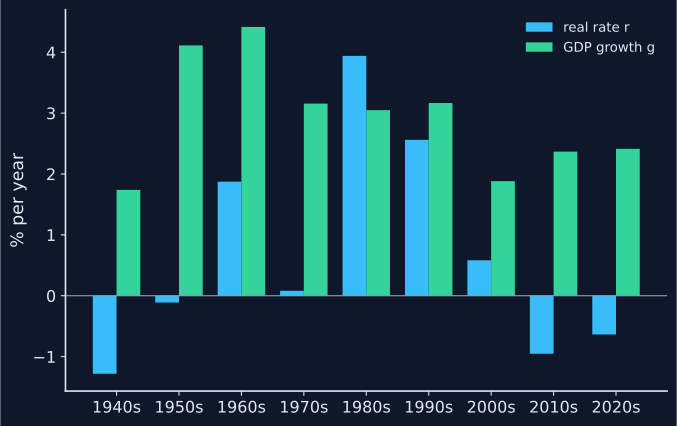
The safe real rate has mostly been below growth

Real T-bill rate vs real GDP growth, US decade averages

Source: FRED (BEA, Federal Reserve Board), snapshot 2026-10-15 · the data lab

With the safe rate, r > g in only 19% of years. But the model’s r is the return on capital.

Mean r − g about −2.1 points, 1948–2025. Which r you measure changes the answer.

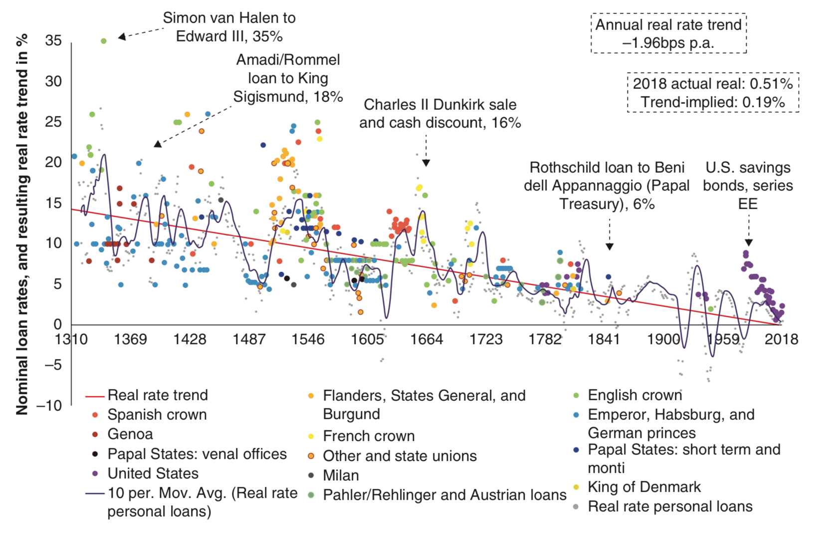
Case study: does r > g make inequality explode?

Real interest rates 1317–2018 (Schmelzing 2019), as reproduced in the chapter

In the model \(r = \rho > n = g\) on the balanced growth path: \(r > g\) is efficiency, not explosion.

Piketty’s fundamental force for divergence. Caveats: human capital; social mobility (Acemoglu and Robinson 2015, whose regressions find r − g does not explain historical top-income shares); factor shares.

If labour is hard to replace, its share can rise as capital grows

\[\frac{wL}{Y} = \alpha\left(\frac{AL}{Y}\right)^{\frac{\varepsilon-1}{\varepsilon}}\]

CES technology: with an elasticity of substitution \(\varepsilon < 1\), labour becomes more essential as the economy grows. Cobb–Douglas (\(\varepsilon = 1\)) keeps the share constant at \(\alpha\).

Whether r > g concentrates income depends on technology, not on r and g alone.

Book eqs. 3.22–3.26. This is one way the Piketty mechanism can be undone.

Case study: the social discount rate decides climate policy

• The Stern Review urged sharp, immediate emission cuts
• Nordhaus (2007): its conclusions hinge on a near-zero discount rate, inconsistent with market real rates and saving rates
• In the model, \(f'(k^*) = \rho\): steady-state capital is very sensitive to \(\rho\)
• Ramsey thought discounting future utility unethical: who should choose \(\rho\)?

The positive question (what do markets reveal?) differs from the normative one (what should a planner use?).

Case study 2 in the guide. Elasticity of k* to rho is −1/alpha = −1.5 with the illustrative alpha.

Optimal saving changes levels, not long-run growth

On the balanced growth path, \(k^*\) and \(y^* = f(k^*)\) are constant: no growth per person.

Diminishing returns stop accumulation once \(f'(k)\) falls to \(\rho\).

Long-run growth needs technology: that is where the next chapters go.

“Do we have growth after all? Not really.”

The tempting mistake — and the correction

Objection. If households become more patient and save more, they must consume less forever.

Response. Consumption falls only on impact. The new steady state has more capital and more consumption.

Quiz item 3.

A second objection: optimal saving rules out oversaving everywhere

Objection. Since optimisers never oversave, dynamic inefficiency is a Solow curiosity.

Response. True for an infinitely-lived planner. With overlapping generations (Chapter 8), markets can accumulate capital beyond the golden rule.

The outline’s second Devil’s-advocate leaf. The NGM’s single household hides intergenerational conflict.

Key takeaways

• Euler equation: \(\dot c / c = \sigma[f'(k) - \rho]\); σ looks small in the data
• Modified golden rule: \(f'(k^*) = \rho\), so no oversaving
• Saddle path: the transversality condition selects the unique path
• Shocks: permanent shifts move the loci; consumption jumps, capital follows
• Policy: \(r > g\) is not destiny; the discount rate is a choice

Point to the guide’s case studies, exercises 3–5 and the data lab’s Your-turn tasks.

Walk the map once more: Act I the question, Act II the model, Act III so what.

Optimal saving reshapes the path to the steady state — not long-run growth.