Chapter 3 — Does consumption grow faster when interest rates are high? And is r > g?
The question. The Euler equation says consumption grows when the return on saving exceeds impatience, \(\dot c / c = \sigma(r - \rho)\). In the data, does consumption grow faster when real interest rates are high? And Piketty’s worry: is the return \(r\) above the growth rate \(g\)?
What the model predicts. A positive relationship between consumption growth and the real interest rate, with slope equal to the elasticity of intertemporal substitution \(\sigma\). And, on the balanced growth path, \(r = \rho > n = g\): r above g.
What you’ll do. Meet the data → explore → confront the model → estimate \(\sigma\) → replicate two classics (Hall’s 1988 estimate; \(r\) versus \(g\)).
TipData literacy: growth rates, real rates and frequencies
Growth as log differences.\(100 \times \Delta \ln c_t\) is (almost exactly) the percentage growth rate. Logs make growth rates additive over time.
Real versus nominal. The model’s \(r\) is a real return. We use the ex-post real rate: the T-bill rate minus the inflation that actually happened. Savers decide on the ex-ante rate, using expected inflation, so this is a proxy.
Changing frequency. Consumption and GDP are quarterly, the T-bill rate monthly. Averaging to annual data reduces noise, at the cost of blurring timing (“time aggregation”), which is one of Hall’s (1988) concerns.
Explore
Tip🔮 Predict, then look
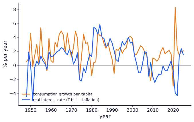
If the Euler equation holds with a sizeable \(\sigma\), consumption growth should rise and fall with the real interest rate. Before you look: do you expect the two lines below to move closely together?
What the data show. Only loosely. Their correlation is 0.22. Consumption growth is remarkably stable, while the real rate swings from deeply negative (high-inflation years) to strongly positive (the early 1980s).
Figure 1: US consumption growth per capita and the ex-post real 3-month T-bill rate, annual, % per year. Source: FRED (BEA, Federal Reserve Board), snapshot 2026-10-15.
Two features stand out. First, consumption growth averages 2.1% per year and rarely turns negative outside recessions. Second, the real rate was negative in the inflationary 1970s and again after 2008, years in which consumption kept growing. That is the first hint of trouble for a large \(\sigma\).
Confront the model
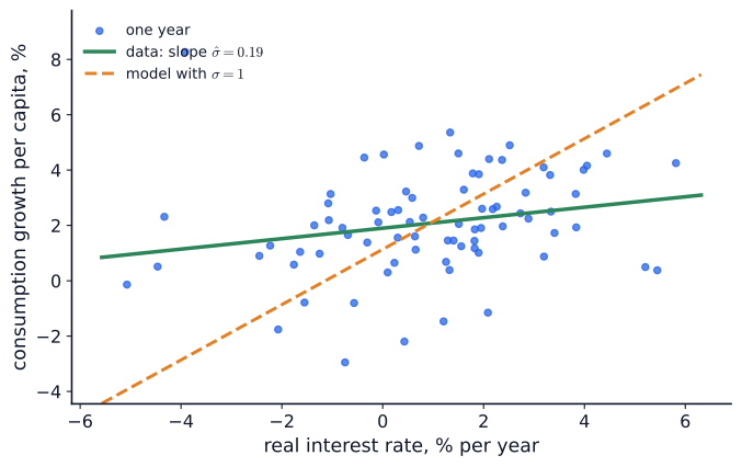
The model predicts points lying along a line of slope \(\sigma\). The orange dashed line shows what \(\sigma = 1\) (log utility, the guide’s illustrative value) would imply, drawn through the sample means. The green line is the best fit to the data.
Figure 2: Consumption growth against the real interest rate, US annual data. The data’s slope (green) is far flatter than σ = 1 would imply (orange, dashed). Source: FRED (BEA, Federal Reserve Board), snapshot 2026-10-15.
The direction is right, since higher real rates go with slightly faster consumption growth. The strength is not: the cloud is nearly flat. Before reading on, list three reasons why the simple Euler equation might fit poorly. Then compare your list with the caveats below.
Estimate
Regress consumption growth on the real rate, \(\;100\,\Delta\ln c_t = a + \sigma\, r_t + \varepsilon_t\), with standard errors robust to autocorrelation (HAC):
The estimated elasticity of intertemporal substitution is \(\hat\sigma =\) 0.19 (standard error 0.12). Its 95% confidence interval, [-0.05, 0.43], includes zero, and the real rate explains only 5% of the variation in consumption growth.
Why the fit is weak. These caveats matter as much as the number:
The ex-post real rate mismeasures the ex-ante rate savers actually face.
The T-bill rate is a safe return, not the return on capital \(f'(k)\) in the model.
Some households are liquidity-constrained and simply consume their income.
Habits and adjustment costs smooth consumption.
Annual averaging blurs timing.
Consumption and interest rates are both endogenous: a regression is not an experiment.
Replicate a classic
1. Hall (1988): is intertemporal substitution weak? Robert Hall asked whether a higher real interest rate induces households to postpone consumption. In post-war US data, he observed, consumption growth was almost steady while expected real returns changed, so he concluded that intertemporal substitution is weak. If it were strong, consumption growth would have moved with returns. With a simple method and data up to 2025, our estimate of 0.19 points the same way. This is a qualitative replication of one of the most debated facts in macroeconomics.
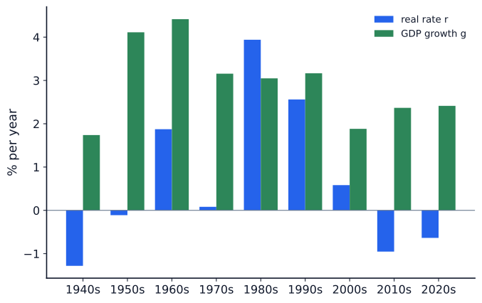
2. Is r > g? The chapter shows Schmelzing’s eight centuries of real rates, declining but mostly above growth “at least until very recently”. What do post-war US data say for the safe real rate against aggregate real GDP growth (the \(g\) in Piketty and in the dynamic-efficiency condition)?
Code
def draw(ax, c): x = np.arange(len(dec)); w =0.38 ax.bar(x - w /2, dec.r, w, color=c["blue"], label="real rate r") ax.bar(x + w /2, dec.g, w, color=c["green"], label="GDP growth g") ax.axhline(0, color=c["muted"], lw=0.8) ax.set_xticks(x, [f"{d}s"for d in dec.index]) ax.set_ylabel("% per year") ax.legend(loc="upper right", fontsize=10)keygraph(draw, "rg", prefix="datalab")
Figure 3: The ex-post real 3-month T-bill rate (r) and aggregate real GDP growth (g), US decade averages, % per year (the 1940s bar covers 1948–49 only). Source: FRED (BEA, Federal Reserve Board), snapshot 2026-10-15.
Over 1948–2025, the safe real rate averaged 2.1 percentage points below growth, and exceeded growth in only 19% of years, mostly the high-rate 1980s. So, with the safe short-term rate, post-war US data mostly show \(r < g\). Only the 1980s are an exception. Schmelzing’s series is different: global, long-term rates over eight centuries, which were mostly above growth until their long decline brought them down. Different rates, places and periods give different pictures. Above all, the \(r\) in Piketty’s argument and in the model (\(r = f'(k)\)) is the return on capital, which includes risk and is well above the T-bill rate. Which \(r\) you measure changes the answer.
Your turn
🟢 In the time-series chart, find two periods in which the real rate was negative yet consumption kept growing. What does the Euler equation predict for those years, and why might households not behave that way?
Estimate \(\sigma\) by instrumental variables, using lagged rates and inflation as instruments (a standard fix for the timing problems in this regression).
Replace the ex-post rate with an ex-ante rate based on the University of Michigan inflation expectations series (fetched live; citation required).
Repeat the r–g comparison with a 10-year bond rate.
What we learned
Direction yes, strength no. Consumption growth rises with the real rate, but weakly. The estimated \(\sigma\) is small and imprecise, in line with Hall’s (1988) conclusion that intertemporal substitution is weak.
Which r matters. The safe real rate has mostly been below GDP growth in the post-war US, while the model’s (and Piketty’s) \(r\) is the return on capital. Comparisons of \(r\) and \(g\) must say which return they mean.
Limits. Ex-post rates, aggregation, liquidity constraints and endogeneity all blur the test. A simple regression cannot identify \(\sigma\) cleanly.
For policy. A small \(\sigma\) means interest-rate changes move consumption only modestly through the intertemporal channel (monetary policy, Chapters 19–21). And \(r < g\) for safe rates eases government debt dynamics (Chapters 17–18).
Data sources and licences
U.S. Bureau of Economic Analysis, Real personal consumption expenditures per capita [A794RX0Q048SBEA], Personal consumption expenditures: chain-type price index [PCECTPI] and Real gross domestic product [GDPC1]. Board of Governors of the Federal Reserve System, 3-month Treasury bill secondary market rate [TB3MS]. All retrieved from FRED, Federal Reserve Bank of St. Louis, on 2026-10-15. Public domain. Snapshots are in data/fred/ and listed on the data page.
# Refresh from source (optional): fetch today's data instead of the dated snapshots (no API key needed).import pandas as pdbase ="https://fred.stlouisfed.org/graph/fredgraph.csv?id="q = pd.read_csv(base +"A794RX0Q048SBEA,PCECTPI", parse_dates=["observation_date"])gdp = pd.read_csv(base +"GDPC1", parse_dates=["observation_date"])tb = pd.read_csv(base +"TB3MS", parse_dates=["observation_date"])a = annual(q, gdp, tb) # then re-run the cells above