Act I — The Question

How much should a society save?

Solow handed households a saving rate — what if they chose it?

In the Solow model, households save a fixed fraction of income, whatever happens.

Real households decide: consume today, or save and consume more tomorrow?

Making saving a choice turns a growth model into a model of optimal behaviour.

Open with the gap the chapter fills. Solow is mechanical: no one chooses anything, so we cannot say whether the outcome is good or bad. Ramsey (1928), revived by Cass and Koopmans in the 1960s, lets saving be chosen. That is the first step towards modern dynamic macroeconomics.

The naive answer — save enough to maximise consumption forever — is wrong

Solow’s golden rule

• pick the capital stock that maximises steady-state consumption
• ignores what it costs to get there

Ramsey’s optimum

• maximise discounted lifetime utility
• counts the sacrifices on the way

Optimal saving weighs the transition, not just the destination.

Many students think “optimal” means “the most consumption in the long run”. The golden rule does that. But reaching it requires years of extra saving, and those sacrifices happen sooner, when they weigh more. We’ll see the optimum stops short of the golden rule.

Where we’re going

• The question: how should households split income between today and tomorrow?
• The model: the Euler equation, the steady state, and the path to it
• So what: what the data say, inequality (\(r > g\)), and why growth still needs technology

Agenda from the guide’s learning objectives: explain the Euler equation, find the steady state, predict the response to a change in patience.

Two kinds of variables: capital is sticky, consumption can jump

Capital \(k\) — the state

• built by past saving
• changes only gradually

Consumption \(c\) — the control

• chosen freely each instant
• can jump when news arrives

When something changes, consumption absorbs the surprise and capital follows.

This distinction decides every dynamic result in the chapter. Keep it in mind for the shock slides. Also define rho (impatience, the rate of time preference) and sigma (willingness to shift consumption over time) here, or on the next slides.

Act II — The Model

Optimal saving, step by step

Households maximise discounted utility of everyone alive

\[\int_0^\infty u(c_t)\, e^{nt} e^{-\rho t}\, dt\]

Utility from consumption per person, counted for a population growing at rate \(n\), and discounted at the rate of time preference \(\rho > n\).

rho greater than n is needed: otherwise future generations’ larger numbers outweigh discounting, and the household would postpone consumption forever. No solution.

Capital grows by what output leaves after consumption

\[\dot k_t = f(k_t) - n k_t - c_t\]

Output \(f(k)\) is consumed or invested; \(nk\) equips the newcomers (“capital widening”). No depreciation, as in the chapter.

This equation of motion makes the problem dynamic: saving today is capital tomorrow.

Per-capita resource constraint, book eq. 3.5. Capital is the state variable: it cannot jump.

The Euler equation: consumption grows when saving pays more than impatience costs

\[\frac{\dot c_t}{c_t} = \sigma\,\big[f'(k_t) - \rho\big]\]

Save one more unit: it earns \(f'(k)\) but you value the future less by \(\rho\). If the return wins, consume more later than now. \(\sigma\) sets how strongly you respond.

Possibly the most important equation in macroeconomics: every intertemporal choice in the book is a variation on it.

The Keynes–Ramsey rule, book eq. 3.15. Intuition first: postpone a unit of consumption, it becomes capital and yields f’(k); but you discount it at rho. sigma is the elasticity of intertemporal substitution.

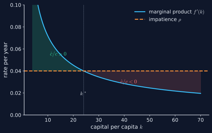
Consumption grows to the left of k*, where capital’s return beats impatience

The Euler equation in one picture (illustrative parameters)

The blue curve is the marginal product, falling because of diminishing returns. The dashed line is rho. Where the curve is above the line, consumption grows; below, it shrinks. They cross at k-star.

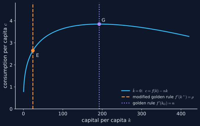
Optimal saving stops short of the golden rule

The kdot = 0 locus peaks at the golden rule; the optimum E lies to its left (illustrative)

Because the future is discounted (\(\rho > n\)), it is not worth building the consumption-maximising capital stock.

The hump is every possible steady state. G maximises steady-state consumption. E, the optimum, has much less capital: with the illustrative parameters about 24 versus 192.

The modified golden rule pins the steady state

\[f'(k^*) = \rho \;>\; n = f'(k_G) \quad\Longrightarrow\quad k^* < k_G\]

Optimal capital: its return equals impatience. Golden rule: its return equals population growth. Since \(\rho > n\), the optimum has less capital.

Optimal saving never oversaves: no dynamic inefficiency.

Book eqs. 3.17–3.18. Contrast with Solow, where oversaving is possible. Chapter 8 returns to whether oversaving can happen with overlapping generations.

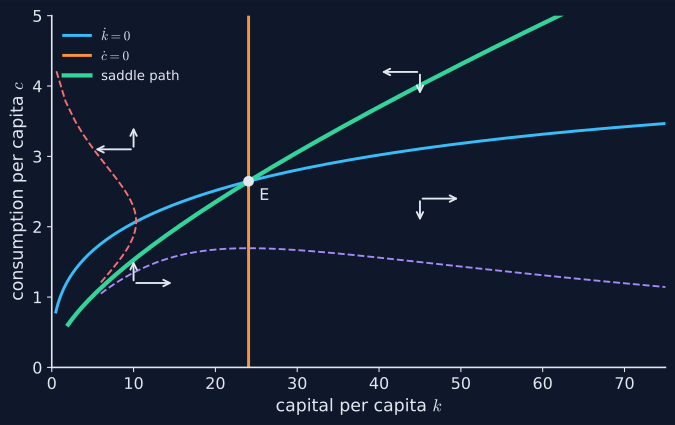
Consumption jumps onto the only road to the steady state

Phase diagram: only the saddle path (green) reaches E (illustrative)

Every other path runs capital out or piles it up forever: not optimal.

Read the arrows: above the hump capital falls; left of the vertical line consumption rises. Only the green saddle path leads into E. Given k0, consumption jumps vertically onto it. Core students need the picture, not the proof.

Twelve lines compute the optimum and the golden rule

import numpy as np                         # arrays and maths
import matplotlib.pyplot as plt            # plotting
alpha, rho, n = 2/3, 0.04, 0.01            # illustrative parameters
f = lambda k: k ** (1 - alpha)             # output per person
k_star = ((1 - alpha) / rho) ** (1 / alpha)    # optimum: f'(k*) = rho
k_gold = ((1 - alpha) / n) ** (1 / alpha)      # golden rule: f'(k_G) = n
k = np.linspace(1, 400, 400)               # grid of capital stocks
plt.plot(k, f(k) - n * k)                  # the kdot = 0 locus
plt.axvline(k_star, ls="--")               # the optimum ...
plt.axvline(k_gold, ls=":")                # ... far left of the golden rule
plt.show()
print(round(k_star, 1), round(k_gold, 1))      # 24.1 192.5

↗ Run the full model in Colab

Self-contained: paste it into a Colab cell. Illustrative parameters (the chapter gives none). The notebook’s Core section simulates the whole transition.

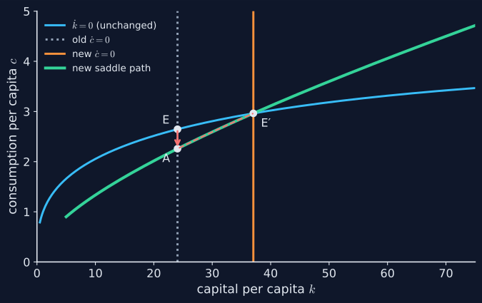
More patience: consumption dips, then climbs to a higher steady state

A permanent fall in ρ: jump from E down to A, then up the new saddle path to E′ (illustrative)

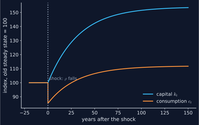
With these numbers consumption falls about 15% on impact, and ends about 12% higher.

Only the cdot = 0 line moves (rho does not enter kdot = 0). Capital cannot jump, so consumption does: down, onto the new saddle path. Numbers from the guide’s key graphs and verification script.

On impact only consumption moves; capital follows gradually

Time paths after the fall in ρ, relative to the old steady state (illustrative)

Same experiment against time. Capital is a stock and rises smoothly. Consumption is a choice: it jumps down, then overtakes its old level.

Act III — So What

What it means for data and policy

US consumption barely responds to interest rates

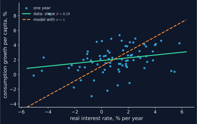
Consumption growth vs the real interest rate, US 1948–2025

Source: FRED (BEA, Federal Reserve Board), snapshot 2026-10-15 · the data lab · notebook

Right direction, weak strength: the estimated slope is about 0.19, far below σ = 1.

The model predicts a line of slope sigma. The data cloud is nearly flat. Hall (1988) concluded that intertemporal substitution is weak. Our simple estimate points the same way. Caveats: ex-post real rate, safe rate, liquidity constraints.

Interest rates beat growth for centuries — yet no plutocracy

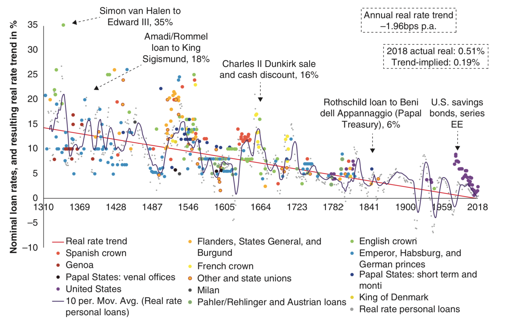
Real interest rates 1317–2018 (Schmelzing 2019), as reproduced in the chapter

In the model \(r = \rho > n = g\): “\(r > g\)” is a property of efficiency, not a recipe for explosion.

Piketty: if r > g, inherited wealth outgrows income. The chapter’s caveats: much capital is human capital, social mobility, and labour may become more essential as economies grow. Schmelzing’s data show rates mostly above growth for centuries without plutocracy.

Optimal saving changes levels, not long-run growth

On the balanced growth path, \(k^*\) and \(y^* = f(k^*)\) are constant: no growth per person.

Diminishing returns still stop accumulation once \(f'(k)\) falls to \(\rho\).

Long-run growth needs technology: that is where the next chapters go.

“Do we have growth after all? Not really.” Endogenising saving was not the missing piece.

The tempting mistake — and the correction

Objection. If households become more patient and save more, they must consume less forever.

Response. Consumption falls only on impact. The extra saving builds capital, and the new steady state has more capital and more consumption.

The guide’s most common misconception, tested in quiz item 3. Point back to the shock graph.

Key takeaways

• The Euler equation: consumption grows when the return on capital beats impatience
• The modified golden rule: \(f'(k^*) = \rho\), so optimal saving never oversaves
• Saddle path: consumption jumps onto the unique path to the steady state
• Shocks: more patience lowers consumption on impact but raises it in the long run
• No long-run growth without technological progress

These match the guide’s key takeaways. Point students to the summary, quiz and data lab.

Walk the map one last time: Act I the question, Act II the model, Act III so what.

Optimal saving reshapes the path to the steady state — not long-run growth.