Where one cross-section runs out

Act I · The tension

This is the capstone chapter. Chapters 1–16 fitted regressions to cross-sections: one observation per unit, no ordering. Real economic data usually has more structure: the same units observed repeatedly (panels), observations ordered in time (time series), and regressors that are themselves chosen (endogeneity). Each structure changes what a slope means and how uncertain it is.

A slope is only as good as the variation behind it

A regression slope compares observations. With one cross-section, the only comparison is across units: big-market teams versus small-market teams, rich countries versus poor ones. Whatever else differs between them rides along in the slope.

This chapter adds two new sources of variation and one warning:

• Panel data: the same unit over time, so we can compare a unit with itself
• Time series: one unit, many periods, so we must respect order and memory
• Causation: no amount of structure helps if the regressor is correlated with the error

The question running through the whole deck: which variation identifies this coefficient, and which standard error is honest about it?

Frame the deck around one question. Pooled OLS uses all variation; fixed effects uses only within-unit variation; first differences uses only period-to-period changes; levels regressions with trending series may be identified by nothing more than two shared trends. The standard error has to match the dependence in the data: clustered for panels, HAC for time series.

Ten stops — click any to jump

Stop	Question	Method	Headline result
17.2	Do wins raise NBA revenue?	Pooled OLS, cluster SEs	+0.0068 per win; SE ×1.81 when clustered
17.3	…holding the team fixed?	Fixed effects (within)	+0.0045 per win (−33%)
17.4	FE or RE?	Random effects, Hausman	concepts (not estimated)
17.4b	Who earns above $60k?	Logit vs LPM	+6.2 pp per year of schooling
17.5	Do long rates follow short rates?	Levels, HAC SEs	\(R^2 = 0.95\); HAC SE ×3.65
17.6	Is the fit spurious?	Correlogram, differences	lag-1 \(\rho\): 0.95 → 0.25
17.6b	How fast is pass-through?	ADL(2,2)	0.74 at once, 0.53 by month 2
17.7	When is a slope causal?	IV & the causal toolkit	links to Ch 13 designs
CS 1	Capital and productivity, 108 countries	Panel FE, two-way FE	capital elasticity 0.71 → 0.44
CS 2	Night lights in 339 municipalities	FE, year effects, FD	population slope +0.34 → −0.82

Every stop follows the same arc: question → method review → code → real output → interpretation → caveats. The stop numbers are links: click one to jump to its divider. Press M for the menu or O for the overview grid.

Stops 17.2–17.6 are the chapter’s worked examples. 17.7 is conceptual in the chapter, so the deck reviews the ideas and points to the Chapter 13 deck for worked causal designs. The two case studies are the chapter’s end-of-chapter tasks, run in full for these slides.

Three data structures, three new problems

Data	Structure	Size	What goes wrong with plain OLS
AED_NBA.DTA	team × season	29 teams, 286 obs.	errors correlated within a team; team traits confound the slope
AED_EARNINGS_COMPLETE.DTA	cross-section, 0/1 outcome	872 workers	a straight line predicts “probabilities” outside \([0,1]\)
AED_INTERESTRATES.DTA	monthly time series	397 months	trends fake a relationship; errors are autocorrelated
Mendez (2020)	country × year	108 × 25	country traits confound capital’s slope
DS4Bolivia	municipality × year	339 × 9	municipality traits confound population’s slope

Each structure needs two fixes: one for the coefficient (which variation) and one for the standard error (which dependence).

The earnings file has 872 workers, as the chapter’s datasets list states, and every result uses all 872. The NBA panel is unbalanced: 28 teams for 10 seasons plus the Bobcats for 6, so 286 team-seasons rather than 29 × 10 = 290.

One estimator, four ways to be honest about uncertainty

SE type	pyfixest syntax	Allows errors to be…	Used for
Default (iid)	(none)	independent, equal variance	benchmark only
Heteroskedasticity-robust	vcov="HC1"	independent, unequal variance	earnings LPM / logit
Cluster-robust	vcov={"CRV1": "teamid"}	correlated within a cluster, independent across	NBA, CS 1, CS 2
HAC (Newey–West)	vcov="NW", vcov_kwargs={"time_id": ..., "lag": 24}	correlated across nearby periods	interest rates

The coefficient never changes with vcov; only SEs, \(t\), \(p\) and CIs do. In this deck the honest SE is 1.8× (NBA), 4× (countries) and 3.65× (rates) the default.

pf.feols is the only estimator for linear models in this chapter; the logit uses statsmodels. The vcov argument changes only inference. Cluster-robust SEs allow any correlation pattern among the observations of one team (or country, or municipality), so they cover both persistent team effects and serial correlation within a team. Newey–West SEs allow correlation that dies out after a chosen number of lags (24 months here).

The thread: which variation identifies the slope?

• Pooled OLS uses all variation: between units and within units over time
• Between variation: differences in unit averages (Knicks vs Bucks)
• Within variation: a unit’s deviations from its own average (the Lakers’ good vs bad seasons). Fixed effects use only this
• Changes (\(\Delta y_t\) on \(\Delta x_t\)): period-to-period movements. First differences and time-series regressions in changes use only this
• Levels of two trending series: may be identified by little more than two shared trends, the classic spurious regression

When a coefficient changes as we move from one kind of variation to another, the change itself is evidence about confounding.

This is the deck’s recurring thread. We will see it four times: NBA (0.0068 pooled → 0.0045 within), countries (capital elasticity 0.71 → 0.44), Bolivian municipalities (population slope +0.34 → −0.82), and interest rates (levels vs changes). Each change is a diagnostic for confounding by something time-invariant (panels) or by a common trend (time series).

Six ideas anchor this chapter

• Panel data: observations indexed by unit \(i\) and time \(t\)
• Within estimator: subtract each unit’s own mean to erase its fixed traits \(\alpha_i\)
• Logit: push \(x'\beta\) through an S-curve so probabilities stay in \([0,1]\)
• AR(\(p\)): regress \(y_t\) on its own past values; persistence and momentum
• ADL: add current and lagged \(x\); cumulative sums of the \(\gamma\)’s trace the dynamic effect
• Hausman test: compares FE and RE; a significant gap rejects RE’s assumption

Each idea answers the same question under harder conditions: what is really driving \(y\)?

These are the chapter’s Key Concepts. One caution: the chapter’s code never estimates random effects or runs the Hausman test; its Key Concepts example quotes RE ≈ 0.0046 and a Hausman χ² ≈ 2.8 (p ≈ 0.10) from fitting RE separately (e.g., with linearmodels). The deck presents the test as a concept (17.4) and reports that check.

Act II-a · Panel data: the same units, again and again

17.2 – 17.4 · pooled OLS, clustering, fixed effects, random effects, logit

Three slides of method, then the NBA example from start to finish: structure, variance decomposition, pooled OLS with three SE types, fixed effects, and the FE-vs-RE choice. The logit example (also in 17.4 of the chapter) closes the act.

17.2 · Do wins raise NBA team revenue?

Panel structure · within vs between · pooled OLS · cluster-robust SEs

Section 17.2: the NBA panel. Tools: describing a panel, decomposing variation, pooled OLS, and why default SEs are wrong when the same team appears ten times.

The question and the panel

Data. NBA team finances, 2001–02 to 2010–11 (AED_NBA.DTA): 29 teams, 286 team-seasons. Revenue is in millions of dollars.

Variable	Meaning	Mean	Range
revenue	team revenue, $ millions	95.7	58.5 – 187.7
lnrevenue	log revenue (outcome)	4.532	4.069 – 5.235
wins	regular-season wins (of 82)	41.0	9 – 67
playoff	1 if the team made the playoffs	0.545	0 – 1
teamid, season	the two panel indexes \(i\) and \(t\)		29 teams × up to 10 seasons

The panel is unbalanced: 28 teams appear in all 10 seasons, the Bobcats in only 6, so \(N = 286\), not \(29 \times 10 = 290\).

Economic question: does winning raise a team’s revenue? A team that wins more sells more tickets, merchandise and playoff games. But big-market teams also have more money to buy winning rosters, so the association could run both ways.

Three ways to use a panel

\[y_{it} = \beta_1 + \beta_2 x_{it} + u_{it}, \qquad i = 1,\dots,n \;(\text{teams}),\; t = 1,\dots,T \;(\text{seasons})\]

• Pooled OLS: ignore the panel structure in estimation; fix the SEs by clustering on \(i\)
• Fixed effects (FE): give each unit its own intercept, \(y_{it} = \alpha_i + \beta_2 x_{it} + \varepsilon_{it}\), and estimate \(\beta_2\) from within-unit changes only
• Random effects (RE): treat \(\alpha_i\) as a random draw, \(u_{it} = \alpha_i + \varepsilon_{it}\), assumed uncorrelated with \(x\); uses a weighted mix of within and between variation

The three estimators differ in which comparison they make, not in arithmetic sophistication.

Pooled OLS treats each team-season as a separate observation for the coefficient but must cluster for inference. FE allows the team effect to be correlated with wins (big markets win more) because it never compares one team with another. RE is more efficient but only consistent if the team effect is unrelated to the regressor.

Code: load the panel and inspect its structure

!pip install -q pyfixest                     # pyfixest is not preinstalled in Colab
import numpy as np                           # numerical operations
import pandas as pd                          # tabular data
import pyfixest as pf                        # OLS / fixed effects with robust and cluster SEs
url = "https://raw.githubusercontent.com/quarcs-lab/data-open/master/AED/AED_NBA.DTA"
data_nba = pd.read_stata(url)                # one row per team-season
print(data_nba.shape)                        # (286, 65): rows, columns
print(data_nba.groupby("teamid").size().value_counts())   # seasons observed per team
data_nba[["revenue", "lnrevenue", "wins", "playoff"]].describe().round(3)

↗ Try it in Colab

Self-contained: paste into an empty Colab cell. The value_counts line reveals the unbalanced panel: 28 teams with 10 seasons, one team (the Bobcats, an expansion franchise) with 6.

Code: split the variation into between and within

\[\underbrace{y_{it}-\bar y}_{\text{overall}} \;=\; \underbrace{\bar y_i-\bar y}_{\text{between}} \;+\; \underbrace{y_{it}-\bar y_i}_{\text{within}}\]

# continues from the previous block
g = data_nba.groupby("teamid")                      # group the rows by team
for v in ["lnrevenue", "wins"]:
    overall = data_nba[v].std()                     # SD over all 286 team-seasons
    between = g[v].mean().std()                     # SD of the 29 team averages
    within = (data_nba[v] - g[v].transform("mean")).std()   # SD of deviations from own mean
    print(f"{v:10s} overall {overall:.4f}  between {between:.4f}  within {within:.4f}")

↗ Try it in Colab

The decomposition is exact for sums of squares. With standard deviations it holds approximately, because the between SD is computed over 29 team means and the within SD over 286 deviations. The chapter computes this only in its cheat-sheet block; it is the first thing to run on any panel.

Output: revenue varies across teams, wins vary within teams

Variable	Overall SD	Between SD	Within SD	Share of variance
lnrevenue	0.2360	0.2127	0.1085	between ≈ 81%
wins	12.44	7.04	10.36	within ≈ 69%

Shares: between variance ÷ overall variance (0.0452 / 0.0557) and within variance ÷ overall variance (107.3 / 154.7).

• Revenue is mostly a team trait: Knicks average $162M, Lakers $150M; Bucks $70M, Grizzlies $74M
• Wins are mostly a season-to-season story: a team’s wins swing more around its own average than team averages differ from each other

Fixed effects throw away 81% of the revenue variance but keep 69% of the wins variance, so the within estimator still has plenty to work with.

The chapter’s “~0.21 between, ~0.11 within, ~0.24 overall” is confirmed exactly. What the chapter does not show is the decomposition for wins, and it matters: if wins had almost no within variation, FE estimates would be very imprecise. Here they have plenty.

The chapter’s team averages (Lakers ≈ $150M, Grizzlies ≈ $74M, a gap of about $77M) match the data: Lakers $150.5M, Grizzlies $73.7M. The largest gap between team averages (Knicks $162.2M vs Bucks $70.5M) is about $92M.

Between and within, side by side

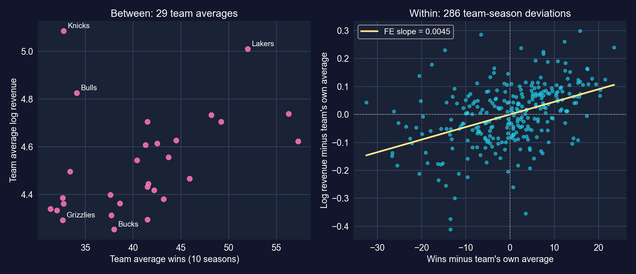
Left: one dot per team (its 10-season averages). Right: each team-season as a deviation from its own team average, with the fixed-effects slope.

The left panel mixes market size with winning (the Knicks earn the most while winning few games). The right panel compares each team only with itself.

Left: across teams the relationship is noisy; the Knicks and Bulls earn a lot without winning much, because of market size. Team-average revenue and team-average wins correlate only 0.40. Right: after removing each team’s averages, more wins than usual go with more revenue than usual. This is exactly the variation fixed effects use; the yellow line is the FE slope, 0.0045.

The pooled picture mixes both comparisons

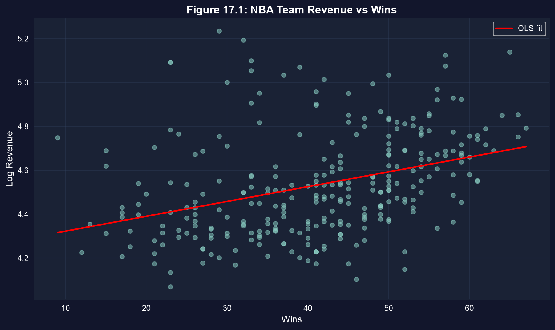
Each dot is a team-season. The pooled OLS line runs through between-team and within-team differences at once.

The pooled slope partly credits winning for market size: big-market teams sit high on the revenue axis whatever their record.

This is the chapter’s Figure 17.1. The positive slope is real as a description, but it bundles two comparisons. The next code block estimates it and asks how to compute its standard error.

Code: pooled OLS with three kinds of standard errors

# continues from the previous block
f_iid = pf.feols("lnrevenue ~ wins", data=data_nba)                 # default (iid) SEs
f_hc1 = pf.feols("lnrevenue ~ wins", data=data_nba, vcov="HC1")     # heteroskedasticity-robust
fit_pool = pf.feols("lnrevenue ~ wins", data=data_nba, vcov={"CRV1": "teamid"})  # by team
for name, f in [("default", f_iid), ("HC1", f_hc1), ("cluster", fit_pool)]:
    print(name, f.coef()["wins"], f.se()["wins"], f.tstat()["wins"])   # same b, new SE
fit_pool.summary()                           # full table with cluster-robust SEs

↗ Try it in Colab

Three fits of the same model. pyfixest’s default for a model without fixed effects is iid SEs. HC1 allows heteroskedasticity across observations. CRV1 with teamid allows any correlation among the ten observations of one team.

Output: same slope, very different uncertainty

SE type	Coef. on wins	SE	\(t\)	\(p\)	95% CI	SE ÷ default
Default (iid)	0.00675	0.00105	6.42	< 0.001	[0.00468, 0.00882]	1.00
HC1	0.00675	0.00102	6.61	< 0.001	[0.00474, 0.00876]	0.97
Cluster by team	0.00675	0.00191	3.54	0.001	[0.00284, 0.01066]	1.81

N = 286 · 29 clusters · \(R^2 = 0.127\) (identical in all three rows)

Heteroskedasticity is not the problem here (HC1 ≈ default). Within-team dependence is: allowing for it widens the SE by 81% and halves the \(t\)-statistic.

Reproduces the chapter’s table: default 0.0011, robust 0.0010, cluster 0.0019, ratio 1.81, which the chapter rounds to about 1.8 (clustering raises the SE by about 80%). Significance survives (t = 3.54, p = 0.001), so clustering corrects the uncertainty without overturning the result.

Why clustering: ten seasons of one team are not ten independent facts

\[\widehat{V}_{\text{CR}}(\hat\beta) = (X'X)^{-1}\Big(\textstyle\sum_{g=1}^{G} X_g'\hat u_g \hat u_g' X_g\Big)(X'X)^{-1}\]

• The middle term sums over clusters \(g\), so every pair of residuals within a team may be correlated; residuals in different teams are assumed independent
• Two sources of within-team correlation: a persistent team effect (the Lakers’ residual is positive every year) and serial correlation (good years follow good years)
• In the limit of perfect correlation, 10 seasons of one team carry the information of 1 observation; the truth lies in between

Clustering must be done at the level where shocks are shared. With \(G = 29\) clusters the \(t\) reference has only \(G - 1 = 28\) degrees of freedom.

The chapter writes the cluster formula with an ellipsis in the denominator; the sandwich form above is the complete version. Practical cautions from the chapter: with fewer than about 30 clusters, cluster-robust SEs can still be too small; the wild cluster bootstrap is the usual refinement (mentioned, not run). Two-way clustering (team and season) allows common season shocks too; its variance is V_team + V_season − V_team×season.

Output: the pooled regression, read correctly

Variable	Coef.	SE	\(t\)	\(p\)	95% CI
Intercept	4.25520	0.09572	44.45	< 0.001	[4.05912, 4.45128]
wins	0.00675	0.00191	3.54	0.001	[0.00284, 0.01066]

N = 286 · CRV1 SEs clustered by teamid (29 clusters) · \(R^2 = 0.127\)

• Log-level model: one more win goes with \(100 \times 0.00675 \approx 0.68\%\) more revenue (a log-point approximation)
• Ten more wins: \(100\,(e^{10 \times 0.00675}-1) = 7.0\%\)
• \(R^2 = 0.127\): wins describe little of the revenue spread, which is mostly team traits

This is an association across and within teams. Teams that win more also tend to be the rich-market teams, so the slope is not yet “the effect of winning”.

Interpretation of a log-level coefficient: 100 × b is the approximate percentage change in revenue per extra win. For larger changes use the exact transformation 100(e^{Δx·b} − 1). The intercept (4.26, i.e. about $70M) is the predicted log revenue at zero wins, an extrapolation outside the data (minimum 9 wins).

17.3 · Fixed effects: compare each team only with itself

Within transformation · LSDV · what FE absorbs · omitted-variable bias

Section 17.3. Fixed effects remove everything about a team that does not change over the decade: market size, arena, brand, ownership, local income (to the extent it is stable).

The fixed-effects model and the within transformation

\[y_{it} = \alpha_i + \beta\,x_{it} + \varepsilon_{it}\]

Average each team’s equation over its seasons and subtract:

\[(y_{it}-\bar y_i) = \beta\,(x_{it}-\bar x_i) + (\varepsilon_{it}-\bar\varepsilon_i)\]

• \(\alpha_i\) disappears: anything constant within a team cannot bias \(\hat\beta\), even if it is correlated with \(x\)
• Same estimate two ways: LSDV (one dummy per team) or de-meaning then OLS
• Price: coefficients on time-invariant regressors cannot be estimated, and only within variation is used

FE swap the assumption “no omitted variables” for the weaker “no omitted variables that change over time within a unit”.

This is the key identifying assumption, often called strict exogeneity: the time-varying error must be uncorrelated with the regressor in every period. Team traits that are fixed over ten seasons (market size, arena, history) are absorbed by alpha_i. Anything that changes over time and drives both wins and revenue (a new star, a new arena, a new TV contract) is not.

Code: fixed effects, and a check by hand

# continues from the previous block
fit_fe = pf.feols("lnrevenue ~ wins | teamid", data=data_nba,
                  vcov={"CRV1": "teamid"})   # "| teamid" = one intercept per team
fit_fe.summary()                             # within estimator, cluster SEs by team
print(fit_fe._r2_within)                     # share of WITHIN-team variation explained
# check: the same slope from OLS on de-meaned data (the within transformation)
data_nba["dm_lnrev"] = data_nba["lnrevenue"] - g["lnrevenue"].transform("mean")
data_nba["dm_wins"] = data_nba["wins"] - g["wins"].transform("mean")
print(pf.feols("dm_lnrev ~ dm_wins - 1", data=data_nba).coef())   # identical slope

↗ Try it in Colab

The vertical bar in the formula tells pyfixest to absorb team fixed effects. The last three lines show that FE is nothing more than OLS on de-meaned data: the slope matches to every digit. (The SEs of the manual regression would need a degrees-of-freedom correction for the 29 estimated means; pyfixest handles that.)

Output: the within-team slope is a third smaller

Variable	Coef.	SE	\(t\)	\(p\)	95% CI
wins	0.00451	0.00084	5.35	< 0.001	[0.00278, 0.00623]

N = 286 · 29 team fixed effects · CRV1 SEs by teamid · within \(R^2 = 0.185\) · manual de-meaned OLS slope: 0.00451

	Pooled OLS	Fixed effects
Coefficient on wins	0.00675	0.00451
Cluster SE	0.00191	0.00084
\(R^2\)	0.127 (overall)	0.185 (within)

Holding the team fixed, the slope falls by 33%, and it is estimated more precisely: removing team effects removed most of the residual noise.

Matches the chapter: 0.0045, SE 0.0008, t 5.35, within R² 0.185. The two R² values are not comparable: one is overall, one is within. Also note that clustering still matters inside FE: the iid SE of the FE slope is 0.00059, so clustering widens it by a factor of 1.42, reflecting serial correlation that the team effects did not remove.

One slope inside each team

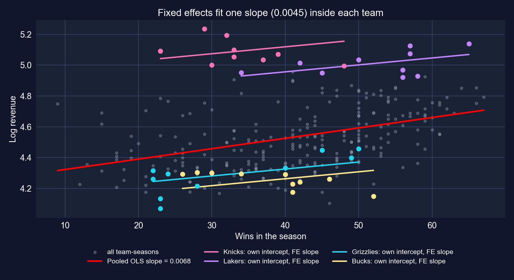
Pooled OLS (red) versus team-specific intercepts with a common fixed-effects slope, for four teams.

Big-market teams (Knicks, Lakers) sit on high lines, small-market teams (Grizzlies, Bucks) on low ones. The pooled line is steeper because it climbs across those lines.

Each colored line uses that team’s own intercept alpha_i and the common FE slope 0.0045. The pooled line connects low-revenue, low-win teams with high-revenue, high-win teams, and that cross-team comparison is where the extra steepness comes from.

Why the slope fell: omitted-variable bias, signed

\[\text{plim}\;\hat\beta_{\text{pooled}} = \beta + \gamma\,\frac{\text{Cov}(\alpha_i, x_{it})}{\text{Var}(x_{it})}\]

• \(\gamma > 0\): the team effect (market, brand) raises revenue
• \(\text{Cov}(\alpha_i, x_{it}) > 0\): rich-market teams also win somewhat more (team-average revenue and wins correlate 0.40)
• So the pooled slope is biased upward: 0.00675 vs 0.00451, a gap of 0.00225

The direction of the change from pooled to FE is exactly what the omitted-variables formula predicts when the omitted trait helps both \(x\) and \(y\).

Same formula as the Phillips-curve case in Chapter 13: bias = (effect of omitted variable on y) × (slope of omitted variable on x). Here the omitted variable is the team fixed effect. FE does not estimate gamma; it removes the term by construction. The 0.40 correlation is between the 29 team averages of log revenue and wins (computed for these slides).

What one more win is worth

• Per win: \(100\,(e^{0.00451}-1) = 0.45\%\) more revenue for the same team
• At the sample mean revenue of $95.7M: about $0.43M per win
• Ten more wins than the team’s usual: \(100\,(e^{10 \times 0.00451}-1) = 4.6\%\), about $4.4M
• The pooled slope would have said 7.0% ($6.7M) for ten wins

Winning pays, but far less than the cross-section suggests. Market size, not the win column, is where most revenue differences come from.

The chapter evaluates the effect for a team with $100M revenue, close to the sample mean (0.45% × $100M = $450K per win, roughly $4.5M for ten wins). The deck uses the sample mean itself ($95.7M; no team-season reaches $200M, maximum $187.7M) and the exact exponential formula, hence $0.43M and $4.4M.

What fixed effects can and cannot fix

Absorbed (time-invariant)

• market size and local income level
• arena, franchise history, brand
• ownership style (if stable)

Not absorbed (time-varying)

• a star arrives, a coach changes, injuries
• new arena or TV contract mid-panel
• league-wide shocks (lockouts, recessions)
• revenue → payroll → wins (reverse causality)

FE make the causal reading more plausible, not guaranteed. A natural next step is season fixed effects, | teamid + season, for league-wide shocks.

Fidelity note. Like the chapter’s model and code (lnrevenue ~ wins | teamid), the FE regression here has no season effects; the chapter says so explicitly. Its within-team illustration (Lakers 2005–06, 34 wins, vs 2009–10, 65 wins) lies inside this sample (2001–02 to 2010–11). Season fixed effects are suggested as an extension, not estimated here.

17.4 · Fixed or random effects?

Random effects · efficiency vs consistency · the Hausman test

Section 17.4. The chapter describes random effects and the Hausman test but does not estimate either: its 17.4 code prints the pooled-vs-FE comparison. The deck therefore reviews the method and reports what the code actually computes.

Random effects: a team effect assumed unrelated to wins

\[y_{it} = \beta_1 + \beta_2 x_{it} + \underbrace{(\alpha_i + \varepsilon_{it})}_{\text{composite error}}, \qquad \alpha_i \sim (0,\sigma_\alpha^2),\;\; \varepsilon_{it} \sim (0,\sigma_\varepsilon^2)\]

• Key assumption: \(\text{Cov}(\alpha_i, x_{it}) = 0\), i.e. the team effect is unrelated to the regressor
• Estimation: feasible GLS, which partially de-means: \(y_{it} - \theta\,\bar y_i\) with \(\theta = 1 - \sqrt{\sigma_\varepsilon^2 / (\sigma_\varepsilon^2 + T\sigma_\alpha^2)}\)
• \(\theta = 0\) gives pooled OLS, \(\theta = 1\) gives FE; RE sits in between and uses some between variation

RE buys efficiency with an assumption. If big-market teams also win more, the assumption fails and RE inherits part of the pooled bias.

The quasi-demeaning formula is the standard textbook RE (GLS) transformation, added here as a method review; the chapter states only “Feasible GLS”. With T = 10 seasons and a large team-effect variance, theta is close to 1, so RE lands close to FE. RE is not estimated in this deck; fitting it separately (linearmodels, as behind the chapter’s Key Concepts example) gives theta ≈ 0.84 and RE ≈ 0.0046, next to FE’s 0.0045.

Pooled, RE, FE: what each one compares

	Pooled OLS	Random effects	Fixed effects
Variation used	between + within, equal weights	within + a fraction \((1-\theta)\) of between	within only
Assumes about \(\alpha_i\)	uncorrelated with \(x\) (and ignored)	uncorrelated with \(x\)	nothing; may correlate with \(x\)
Consistent if \(\alpha_i\) correlates with \(x\)?	no	no	yes
Efficient if it doesn’t?	no	yes	no
Time-invariant regressors?	yes	yes	no
NBA estimate	0.00675	not estimated	0.00451

In observational panels the “no correlation” assumption is rarely credible, so FE is the default and RE needs a justification.

RE is typically defensible when the unit effects are plausibly random with respect to the regressor, for example when the regressor is randomly assigned. In the NBA case, market size almost certainly correlates with the ability to buy a winning roster.

The Hausman test: does RE’s assumption survive?

\[H = (\hat\beta_{FE} - \hat\beta_{RE})'\,\big[\widehat V(\hat\beta_{FE}) - \widehat V(\hat\beta_{RE})\big]^{-1}(\hat\beta_{FE} - \hat\beta_{RE}) \;\sim\; \chi^2_k\]

• \(H_0\): \(\alpha_i\) uncorrelated with the regressors, so both are consistent and RE is efficient: the two estimates should be close
• \(H_a\): correlated, so only FE is consistent: the estimates diverge
• A large \(H\) (small \(p\)) rejects RE; keep FE

The chapter’s code does not run the test; fitting RE separately (as its Key Concepts example reports) gives \(\chi^2 \approx 2.8\), \(p \approx 0.10\): RE is not rejected at 5%, and FE (0.0045) and RE (0.0046) nearly coincide.

The classic Hausman statistic assumes RE is fully efficient under H0, which fails with heteroskedastic or clustered errors; a robust alternative is the correlated-random-effects (Mundlak) test, adding team means of x as regressors. Both are mentioned as standard practice, not estimated.

Fidelity note: the chapter’s code does not estimate RE or run the test; its Key Concepts example quotes RE ≈ 0.0046 and χ² ≈ 2.8 (p ≈ 0.10) from a separate fit, which linearmodels reproduces (classic version: χ² = 2.75, p = 0.097). Practice Exercise 3 (χ² = 25.4) is a hypothetical, not this dataset.

Code: what the chapter’s 17.4 cell actually computes

# continues from the previous block (the chapter's 17.4 code)
comparison_table = pd.DataFrame({
    "Pooled OLS": [fit_pool.coef()["wins"], fit_pool.se()["wins"], fit_pool._r2, fit_pool._N],
    "Fixed Effects": [fit_fe.coef()["wins"], fit_fe.se()["wins"], fit_fe._r2_within, fit_fe._N]
}, index=["Wins Coefficient", "Wins Std Error", "R²", "N"])
print(comparison_table)                      # R² rows differ in kind: overall vs within

↗ Try it in Colab

	Pooled OLS	Fixed effects
Wins coefficient	0.00675	0.00451
Std. error (cluster)	0.00191	0.00084
\(R^2\)	0.127	0.185
\(N\)	286	286

pyfixest focuses on fixed-effects estimation and has no random-effects estimator; the chapter notes this in a code comment. In Python, the linearmodels package provides RandomEffects and a Hausman-type comparison; that is outside this chapter’s toolkit and is not run here.

17.4b · Who earns more than $60,000?

Binary outcomes · linear probability model · logit · marginal effects

The chapter’s 17.4 also introduces nonlinear models through a logit. Different data: a cross-section of workers, no panel structure. The lesson: when y is 0/1, read the model through predicted probabilities and marginal effects.

The question: education, age and the chance of a high income

Data. 872 full-time workers, 2010 (AED_EARNINGS_COMPLETE.DTA). Outcome: dbigearn = 1 if annual earnings exceed $60,000.

Variable	Meaning	Mean
dbigearn	1 if earnings > $60,000 (238 workers)	0.273
education	years of schooling (0–20)	13.85
age	years	43.3

• Linear probability model (LPM): \(\Pr(y=1\mid x) = x'\beta\); slopes are probability changes, but fitted values can leave \([0,1]\)
• Logit: \(\Pr(y=1\mid x) = \dfrac{e^{x'\beta}}{1+e^{x'\beta}}\); always in \((0,1)\), but \(\beta_j\) is in log-odds units

Logit’s marginal effect \(\partial p/\partial x_j = p(1-p)\,\beta_j\) changes with \(p\), so you must say where you evaluate it.

The file has 872 workers, as the chapter’s datasets list states, and all results use 872. The marginal effect is largest at p = 0.5, where it equals β/4, and shrinks toward zero in the tails.

Code: build the binary outcome and fit the logit

!pip install -q pyfixest                      # pyfixest is not preinstalled in Colab
import pandas as pd                           # tabular data
import pyfixest as pf                         # OLS for the linear probability model
from statsmodels.formula.api import logit     # logit with R-style formulas
url = "https://raw.githubusercontent.com/quarcs-lab/data-open/master/AED/AED_EARNINGS_COMPLETE.DTA"
data_earnings = pd.read_stata(url)            # 872 full-time workers, 2010
data_earnings["dbigearn"] = (data_earnings["earnings"] > 60000).astype(int)  # 1 = high earner
print(data_earnings["dbigearn"].mean())       # share of high earners
model_logit = logit("dbigearn ~ age + education", data=data_earnings).fit(cov_type="HC1", disp=0)
print(model_logit.summary())                  # coefficients in log-odds units, robust SEs

↗ Try it in Colab

Self-contained block. The logit is fitted by maximum likelihood; cov_type=“HC1” requests heteroskedasticity-robust (sandwich) standard errors, as in the chapter.

Output: logit coefficients are log-odds, not probabilities

Variable	Coef.	SE	\(z\)	\(p\)
Intercept	−8.0651	0.6914	−11.67	< 0.001
age	0.0385	0.0080	4.85	< 0.001
education	0.3742	0.0366	10.22	< 0.001

N = 872 · share with dbigearn = 1: 0.273 · HC1 SEs · McFadden pseudo-\(R^2 = 0.145\)

• Sign and significance read as usual: older and more educated workers are more likely to earn above $60k
• Size does not: one more year of schooling multiplies the odds by \(e^{0.3742} = 1.45\)
• To talk about probabilities we need marginal effects

A logit coefficient of 0.37 is not “37 percentage points”. It is a change in log-odds.

Pseudo-R² compares the log likelihood with a constant-only model; it is not a share of variance and is typically much lower than OLS R² values. The odds ratio is the cleanest exact reading of a logit coefficient.

Code: marginal effects and the linear probability model

# continues from the previous block
ame = model_logit.get_margeff()               # default at="overall": AVERAGE marginal effects
mem = model_logit.get_margeff(at="mean")      # marginal effects AT THE MEANS of age, education
print(ame.summary()); print(mem.summary())
fit_lpm = pf.feols("dbigearn ~ age + education", data=data_earnings, vcov="HC1")
fit_lpm.summary()                             # slopes are directly probability changes
p_lpm = fit_lpm.predict()                     # LPM fitted "probabilities"
print((p_lpm < 0).sum(), p_lpm.min())         # how many fall below zero?

↗ Try it in Colab

The chapter calls get_margeff() and labels the output as average marginal effects: statsmodels’ default is at=“overall”, which averages each worker’s marginal effect (the AME). Marginal effects at the means need at=“mean”. The deck runs both.

Output: three answers to “one more year of schooling”

Effect on \(\Pr(\text{earnings} > \$60\text{k})\)	education	SE	age	SE
Logit, average marginal effect (get_margeff())	0.0618	0.0047	0.0064	0.0013
Logit, marginal effect at the means (at="mean")	0.0662	0.0062	0.0068	0.0014
Linear probability model (OLS, HC1)	0.0540	0.0050	0.0064	0.0013

LPM: N = 872 · \(R^2 = 0.142\) · 95% CI for education [0.0442, 0.0639]

One more year of schooling raises the probability of earning above $60k by about 6.2 percentage points on average (logit), or 5.4 (LPM). Same sign, similar size.

The chapter reports the average marginal effect of education as about 0.06 (about 0.07 at the sample means) and the LPM coefficient as about 0.05. Exact values: AME 0.062 (what the chapter’s code prints), at the means 0.066, LPM 0.054. Logit and LPM agree on sign and rough size. The formula check: p at the means = 0.229, so 0.229 × 0.771 × 0.3742 = 0.066.

Where the two models part ways

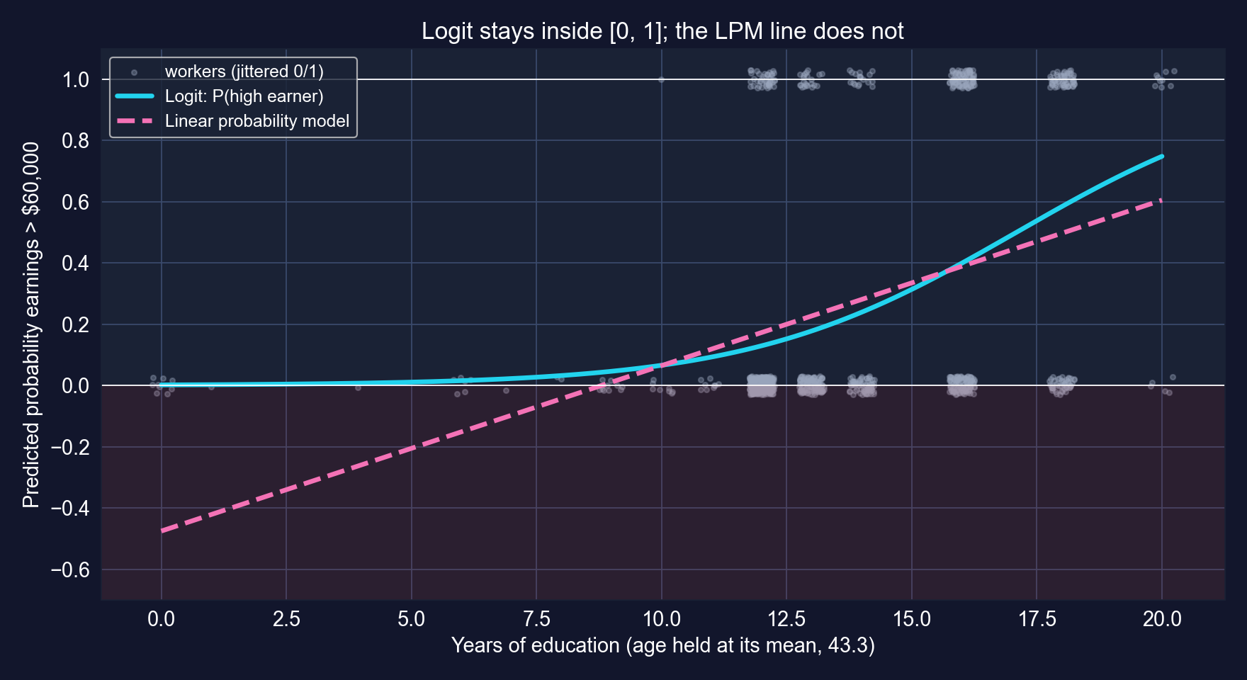
Predicted probability by years of education, age fixed at its mean. Shaded: impossible negative “probabilities”.

In the data, 30 of 872 LPM fitted values are negative (minimum −0.59). Every logit prediction stays between 0.001 and 0.86.

The two curves agree in the middle of the data (12–16 years of schooling): at 16 years both predict about 0.39–0.40. They diverge in the tails, where the LPM line keeps going and the logit flattens. At 20 years the logit predicts 0.75, the LPM 0.61. The negative LPM predictions come from workers with very little schooling. Average marginal effects summarize the curve with one number; the picture shows why one number hides variation.

Reading the logit honestly

• Report marginal effects, and say which: average (AME) or at the means (MEM). They differ here by 0.004
• LPM is a fine first pass for average effects near the middle of the data; use logit (or probit) for predictions and for the tails
• Association, not return to schooling: ability, family background and occupation choice correlate with education and with earnings
• The cut-off is arbitrary: $60,000 discards most of the information in earnings, which the log-earnings regressions of earlier chapters use in full

A binary model changes the scale of the answer, not the identification problem.

This example sits in the panel chapter only because the chapter places nonlinear models in 17.4. Nothing here is a panel. The identification caveats are the same as for any cross-sectional regression of earnings on education.

Act II-b · Time series: order and memory

17.5 – 17.6 · stationarity, spurious regression, HAC, autocorrelation, AR and ADL

One unit (the U.S. Treasury market), 397 months. The panel problems become time problems: shared trends instead of shared team traits, and serial correlation instead of within-cluster correlation.

17.5 · Do long rates follow short rates?

Stationarity · spurious regression · levels with a trend · Newey–West HAC

Section 17.5: the levels regression of the 10-year Treasury rate on the 1-year rate, with a time trend, under default and HAC standard errors.

The question and the data

Data. Monthly U.S. Treasury yields, January 1982 – January 2015: 397 months (AED_INTERESTRATES.DTA).

Variable	Meaning	Mean	Range
gs10	10-year Treasury rate, %	6.19	1.53 – 14.59
gs1	1-year Treasury rate, %	4.69	0.10 – 14.73
dgs10	monthly change in gs10, percentage points	−0.03	−1.43 – 0.78
dgs1	monthly change in gs1, percentage points	−0.04	−1.81 – 0.76

Economic question: how much of a move in short rates (which the Fed influences) passes through to long rates (which matter for mortgages and investment)?

The expectations hypothesis says long rates reflect expected future short rates, plus a term premium. If so, short-rate moves should pass through to long rates, but less than one-for-one, because a 1-year move changes only part of the expected 10-year path.

Three time-series ideas to keep in view

• Autocorrelation at lag \(k\): \(r_k = \dfrac{\sum_{t=k+1}^{T}(y_t-\bar y)(y_{t-k}-\bar y)}{\sum_{t=1}^{T}(y_t-\bar y)^2}\). Today resembles yesterday
• Stationarity: mean, variance and autocorrelations do not change over time. Trending series are non-stationary
• Spurious regression: regress one trending series on another and you get a high \(R^2\) and huge \(t\)-statistics even with no structural link

With trending data a large \(R^2\) is a warning, not a reward. Two cures: difference the data, or keep levels and use HAC standard errors (and think hard).

Many macro series behave like random walks with drift; their levels wander and their changes are roughly stationary. Spurious regression (Granger and Newbold) is the time-series analogue of confounding by a common factor: here the common factor is time itself.

Both rates drift down from 14% to near zero

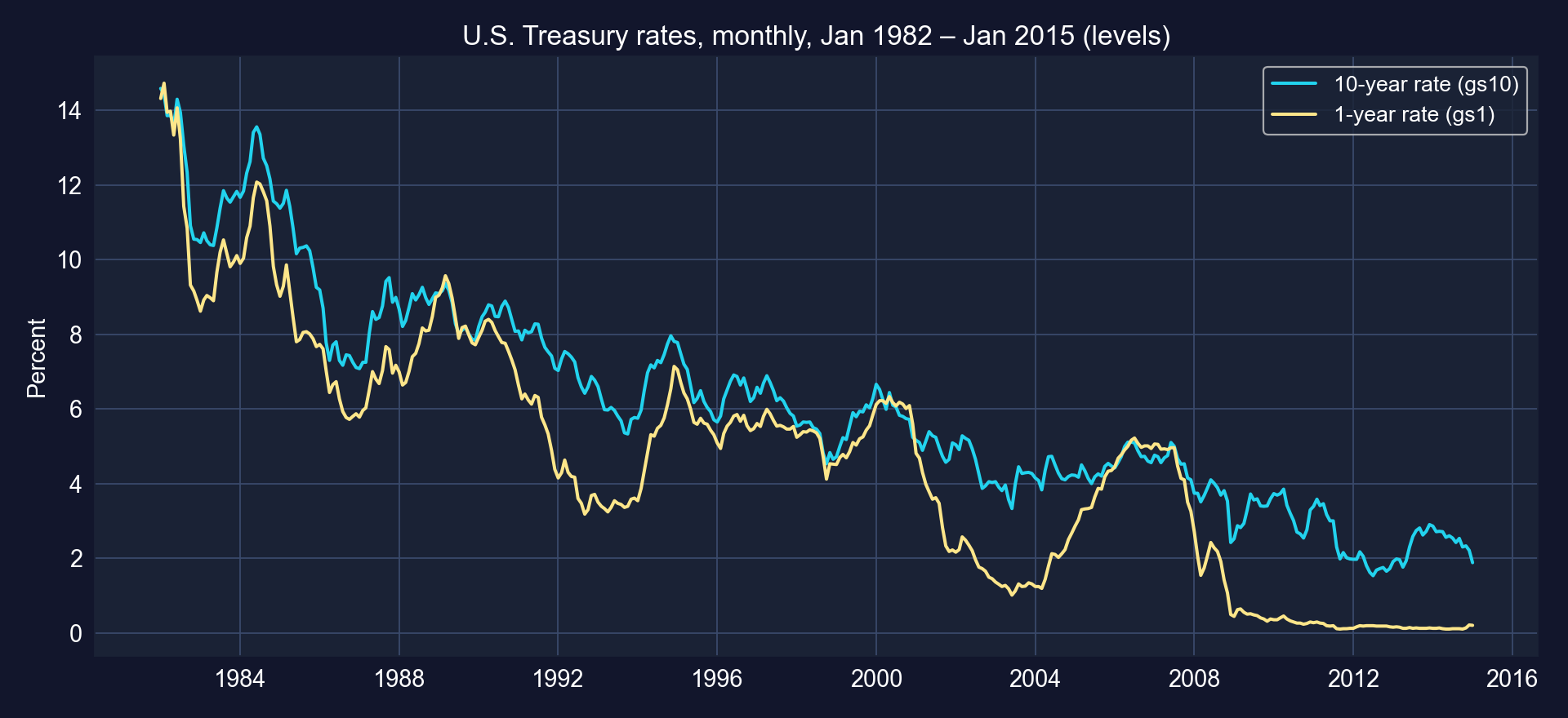
Monthly 10-year and 1-year Treasury yields, 1982–2015.

Over 33 years both rates fall by more than ten points. Any regression of one level on the other will partly fit this shared downward drift. In levels the two series correlate 0.95.

Notice also the late period: after 2008 the 1-year rate is pinned near zero (the zero lower bound) while the 10-year rate keeps moving. A single linear relationship across 1982–2015 also assumes the relationship is stable through very different monetary regimes.

Code: the levels regression, with default and HAC SEs

!pip install -q pyfixest                     # pyfixest is not preinstalled in Colab
import numpy as np                           # numerical operations
import pandas as pd                          # tabular data
import pyfixest as pf                        # OLS with default / HAC standard errors
url = "https://raw.githubusercontent.com/quarcs-lab/data-open/master/AED/AED_INTERESTRATES.DTA"
data_rates = pd.read_stata(url)              # 397 months, Jan 1982 – Jan 2015
data_rates["time"] = np.arange(len(data_rates))              # linear time trend 0, 1, 2, ...
fit_levels = pf.feols("gs10 ~ gs1 + time", data=data_rates)   # default SEs
fit_levels_hac = pf.feols("gs10 ~ gs1 + time", data=data_rates, vcov="NW",
                          vcov_kwargs={"time_id": "time", "lag": 24})   # Newey–West, 24 lags
fit_levels_hac.summary()                     # same coefficients, HAC SEs

↗ Try it in Colab

Self-contained. Including a linear time trend lets the regression absorb a common linear drift, but not wandering, non-linear trends. HAC with 24 lags allows errors to be correlated over two years of monthly data.

Output: a near-perfect fit, and SEs that were 3.6× too small

Variable	Coef.	Default SE	Default \(t\)	HAC SE	HAC \(t\)	HAC ÷ default
Intercept	5.8994	0.2254	26.17	0.6640	8.89	2.95
gs1	0.5076	0.0221	22.92	0.0808	6.28	3.65
time	−0.0106	0.0006	−16.69	0.0018	−5.79	2.88

N = 397 · \(R^2 = 0.947\) · HAC: Newey–West, 24 lags · HAC 95% CI for gs1: [0.3488, 0.6663]

Holding a linear trend fixed, a 1-point higher short rate goes with a 0.51-point higher long rate. The fit looks superb, but the residuals are highly persistent, so default SEs overstate precision more than threefold.

Matches the chapter: R² around 0.95 and a HAC SE more than three times the default (3.65×). The time coefficient says the long rate drifted down by about 0.011 points per month (about 0.13 per year) beyond what the short rate explains.

The chapter later claims the “long-run” levels coefficient is “≈ 0.90–0.95”. With the trend it is 0.51; without the trend (the chapter’s cheat-sheet regression gs10 ~ gs1) it is 0.84, with R² 0.909. Neither is 0.90–0.95.

How HAC standard errors work

\[\widehat V_{\text{HAC}} = (X'X)^{-1}\Big[\hat\Omega_0 + \sum_{\ell=1}^{L} w_\ell\,\big(\hat\Omega_\ell + \hat\Omega_\ell'\big)\Big](X'X)^{-1}, \qquad w_\ell = 1 - \frac{\ell}{L+1}\]

• \(\hat\Omega_\ell = \sum_t \hat u_t \hat u_{t-\ell}\, x_t x_{t-\ell}'\): the covariance of scores \(\ell\) months apart
• Bartlett weights \(w_\ell\) shrink distant lags; \(L\) is chosen by the analyst (here 24 months)
• HAC fixes the standard errors; it does not fix a spurious coefficient

HAC is to time series what clustering is to panels: same sandwich, different idea of which errors may be correlated.

The Newey–West estimator is the cluster-robust sandwich with a different middle: instead of summing within clusters, it sums cross-products of nearby periods with declining weights. Choosing L: rules of thumb such as 0.75·T^(1/3) give about 5.5 for T = 397; the chapter chooses 24 (two years) to be conservative given the strong persistence.

17.6 · Autocorrelation: is the levels fit spurious?

Correlogram · consequences · first differencing

Section 17.6: diagnose the residuals of the levels regression, then re-estimate in changes.

Autocorrelation: what it breaks and how to see it

• Consequences: OLS coefficients stay unbiased (if the regressors are exogenous), but default SEs are wrong, usually too small, and \(t\)-tests over-reject
• Detect: the correlogram of residuals; the Breusch–Godfrey LM test; the Durbin–Watson statistic for AR(1) errors
• Respond: HAC SEs; model the dynamics (AR, ADL); or first-difference non-stationary series

A slowly decaying correlogram is the fingerprint of a non-stationary, near-unit-root error.

The chapter imports acorr_breusch_godfrey but never runs it; the deck relies on the correlogram, as the chapter’s code does. Approximate 95% band for a single autocorrelation under white noise: ±1.96/√T = ±0.098 here.

Code: residual autocorrelations of the levels regression

# continues from the previous block
from statsmodels.tsa.stattools import acf             # autocorrelation function
from statsmodels.graphics.tsaplots import plot_acf    # correlogram plot
data_rates["uhatgs10"] = fit_levels._u_hat            # residuals of the levels regression
acf_resid = acf(data_rates["uhatgs10"].dropna(), nlags=10)   # lags 0..10
for k in range(11): print(k, round(acf_resid[k], 3)) # lag-1 ≈ 0.95
plot_acf(data_rates["uhatgs10"].dropna(), lags=24, alpha=0.05)  # with a 95% band

↗ Try it in Colab

The residuals of the levels-plus-trend regression are what the trend did not absorb. If they wander, the regression has not captured a stable relationship.

Output: the residuals barely forget

Lag	\(r_k\)
1	0.953
2	0.888
3	0.830
4	0.769
5	0.709
8	0.538
10	0.425

95% band: ±0.098

Correlogram of the levels-regression residuals, lags 1–24.

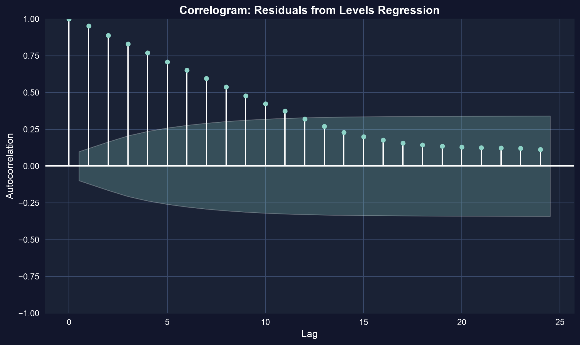
Still 0.42 after ten months. Errors this persistent mean the 397 months carry far less independent information than 397 observations, which is why HAC SEs were 3.65× larger.

Matches the chapter: lag 1 = 0.95, lag 10 = 0.42. Every bar is far outside the band. This is the signature of non-stationary (or near unit-root) residuals: the levels relationship may be partly spurious.

First differences: compare changes with changes

\[\Delta y_t = y_t - y_{t-1}, \qquad \Delta\text{gs10}_t = \beta_1 + \beta_2\,\Delta\text{gs1}_t + u_t\]

• Differencing removes a stochastic trend and any linear trend (it becomes the intercept)
• The question changes: “when short rates move this month, how much do long rates move?”
• Cost: long-run level information is discarded; only month-to-month variation identifies \(\beta_2\)

The time-series cousin of fixed effects: drop the persistent component, keep the changes.

The analogy is exact for two-period panels: first differences and fixed effects coincide when T = 2. In both cases, a component that does not change (a team’s market, a series’ level) is removed so that it cannot confound the slope.

Monthly changes: no trend, centred on zero

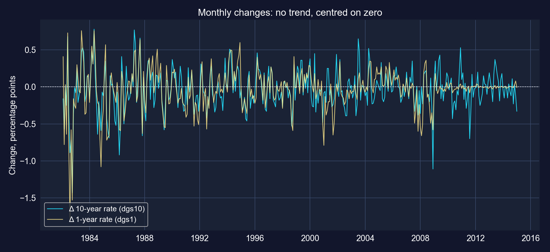
Monthly changes in the 10-year and 1-year rates, 1982–2015.

The changes look stationary: no drift, a constant mean near zero, but bursts of volatility (early 1980s, 2008), a reminder to use robust SEs.

Volatility clustering is a form of heteroskedasticity over time. The chapter estimates the changes regression with default SEs; HAC SEs for the same regression are 0.042 instead of 0.031 for dgs1 (computed for these slides), which changes nothing substantive here (t = 17 instead of 23).

Code: the regression in changes

# continues from the previous block
fit_changes = pf.feols("dgs10 ~ dgs1", data=data_rates)   # regression in first differences
fit_changes.summary()                                    # N = 396 (first month has no change)
uhat_dgs10 = fit_changes._u_hat                          # residuals in changes
acf_dgs10_resid = acf(uhat_dgs10[~np.isnan(uhat_dgs10)], nlags=10)
print(acf_dgs10_resid[1])                                # lag-1 autocorrelation

↗ Try it in Colab

The dataset already contains dgs10 and dgs1, so no differencing is needed in code. The first month is lost because its change is undefined.

Output: changes pass through at 0.72, and the residuals relax

Variable	Coef.	SE	\(t\)	\(p\)	95% CI
Intercept	−0.0064	0.0091	−0.71	0.480	[−0.0243, 0.0115]
dgs1	0.7198	0.0314	22.89	< 0.001	[0.6580, 0.7817]

N = 396 · default SEs (as in the chapter) · \(R^2 = 0.571\) · residual autocorrelation: lag 1 = 0.255, lag 2 = −0.039, lag 3 = 0.061

	Levels + trend	Changes
Slope on the 1-year rate	0.508	0.720
\(R^2\)	0.947	0.571
Residual lag-1 autocorrelation	0.953	0.255

A 1-point change in the short rate goes with a 0.72-point change in the long rate the same month. \(R^2\) falls, but now it is honest.

Matches the chapter’s Key Concept 17.7: residual lag-1 autocorrelation drops from about 0.95 to about 0.25, and the slope in changes is 0.72. Some autocorrelation remains (0.255 is well outside ±0.098), which motivates modelling the dynamics next.

17.6b · How fast do short-rate moves reach long rates?

AR(\(p\)) · ADL(\(p,q\)) · impact and cumulative multipliers

Still section 17.6 in the chapter (Autoregressive Models). The ADL(2,2) is estimated in the chapter’s Key Takeaways code block; the deck runs it as a main result.

Dynamic models: let the past enter the regression

\[\text{AR}(p):\quad y_t = \beta_0 + \alpha_1 y_{t-1} + \cdots + \alpha_p y_{t-p} + u_t\]

\[\text{ADL}(p,q):\quad y_t = \beta_0 + \sum_{j=1}^{p}\alpha_j\,y_{t-j} + \sum_{j=0}^{q}\gamma_j\,x_{t-j} + u_t\]

• \(\alpha_j\): persistence (momentum or reversal) in \(y\) itself
• \(\gamma_0\): impact multiplier, the same-month response to \(x\)
• \(\gamma_0+\gamma_1+\dots\): cumulative distributed-lag multipliers; the long-run multiplier also accounts for the AR terms: \(\sum_j\gamma_j \,/\, (1-\sum_j \alpha_j)\)

Here \(y_t = \Delta\text{gs10}_t\) and \(x_t = \Delta\text{gs1}_t\): an ADL(2,2) in changes.

The long-run multiplier formula is standard for stable ADL models: after a permanent unit change in x, y settles where y = (Σγ/(1−Σα))·x. With y and x in changes, this is the long-run response of the change in the long rate to a sustained change in the change of the short rate. Students should mainly read the impact and cumulative sums.

Code: build lags and fit the ADL(2,2)

# continues from the previous block
for k in [1, 2]:                                       # lags with .shift(k)
    data_rates[f"dgs10_lag{k}"] = data_rates["dgs10"].shift(k)
    data_rates[f"dgs1_lag{k}"] = data_rates["dgs1"].shift(k)
fit_adl = pf.feols("dgs10 ~ dgs10_lag1 + dgs10_lag2 + dgs1 + dgs1_lag1 + dgs1_lag2",
                   data=data_rates)                    # ADL(2,2), N = 394
fit_adl.summary()                                      # default SEs, as in the chapter
c = fit_adl.coef()                                     # cumulative pass-through:
print(c["dgs1"], c["dgs1"] + c["dgs1_lag1"], c["dgs1"] + c["dgs1_lag1"] + c["dgs1_lag2"])
print(acf(pd.Series(fit_adl._u_hat).dropna(), nlags=1)[1])   # residual lag-1 autocorrelation

↗ Try it in Colab

Three months are lost to the lags (one for the difference, two for the second lag), leaving 394. The code is the chapter’s Key Takeaways cheat-sheet block.

Output: strong impact, partial reversal, positive momentum

Variable	Coef.	SE	\(t\)	\(p\)	95% CI
Intercept	−0.0067	0.0088	−0.76	0.447	[−0.0239, 0.0106]
dgs10_lag1	0.2830	0.0508	5.57	< 0.001	[0.1831, 0.3828]
dgs10_lag2	−0.1021	0.0506	−2.02	0.044	[−0.2015, −0.0027]
dgs1	0.7397	0.0340	21.74	< 0.001	[0.6728, 0.8066]
dgs1_lag1	−0.2588	0.0514	−5.03	< 0.001	[−0.3599, −0.1576]
dgs1_lag2	0.0515	0.0492	1.05	0.296	[−0.0453, 0.1482]

N = 394 · default SEs · \(R^2 = 0.611\) · residual lag-1 autocorrelation 0.008

Same month: 0.74 points of pass-through. Next month a partial reversal (−0.26). The long rate’s own lagged change enters positively (+0.28): momentum, not mean reversion.

These match the chapter’s ADL(2,2) results (own lag ≈ +0.28, γ0 ≈ 0.74, γ1 ≈ −0.26, γ2 ≈ 0.05, two-month multiplier ≈ 0.53, R² ≈ 0.61 vs 0.57 for the static changes regression): momentum in the long rate’s own changes, with a partial reversal of the impact response. HAC SEs (computed for these slides) leave every conclusion unchanged: γ0 t = 14.0, γ1 t = −4.33, γ2 p = 0.26.

Pass-through, month by month

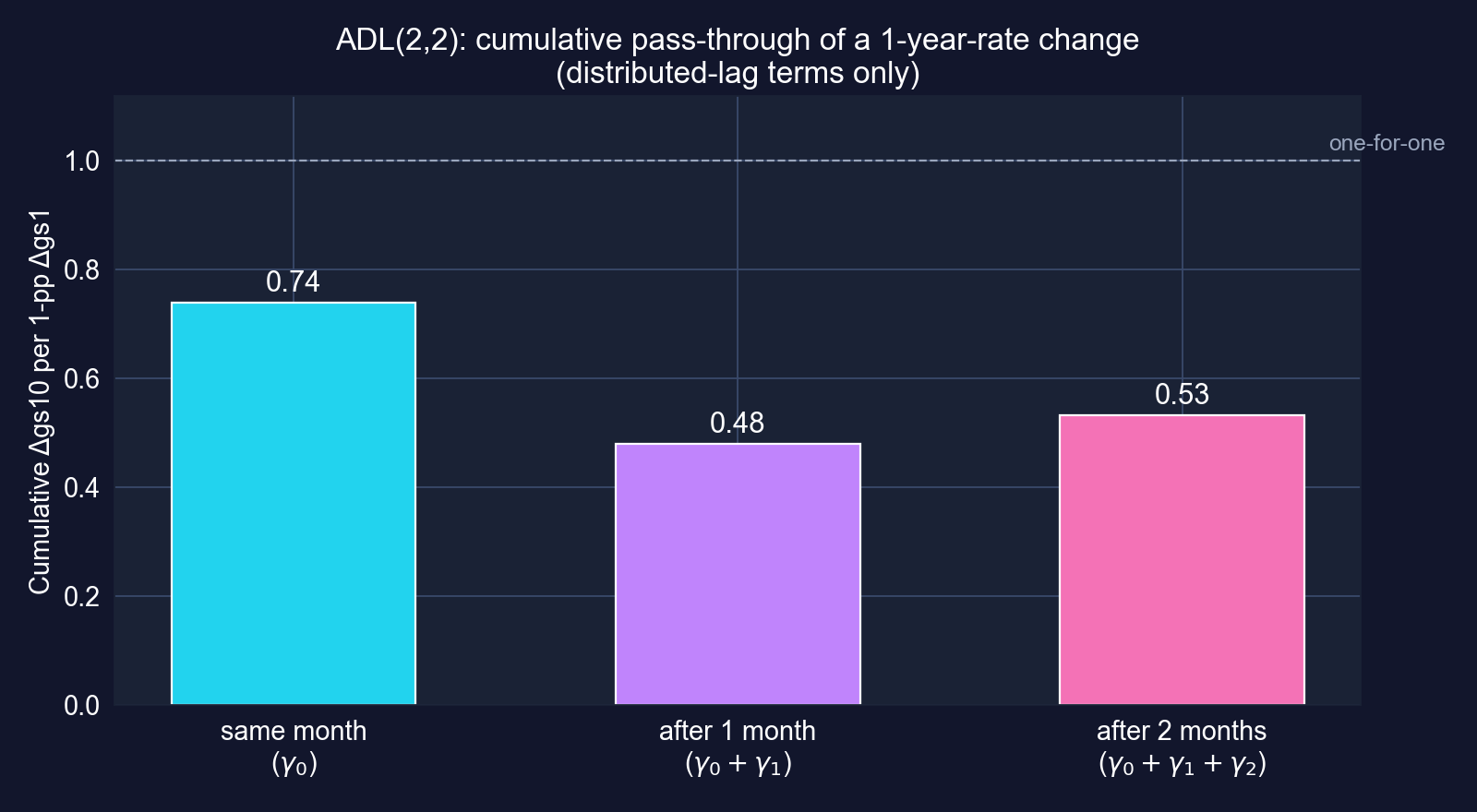
Cumulative distributed-lag multipliers from the ADL(2,2).

About 0.74 of a 1-point short-rate change shows up in the long rate at once; after the partial reversal, 0.53 has passed through within two months.

Cumulative sums of the γ coefficients: 0.740, 0.481, 0.532. Including the autoregressive terms, the long-run multiplier is 0.532 / (1 − 0.283 + 0.102) = 0.65, as in the chapter. All are well below one-for-one, consistent with the expectations hypothesis: a change in the 1-year rate moves only part of the expected path of short rates over ten years.

Did the dynamics soak up the autocorrelation?

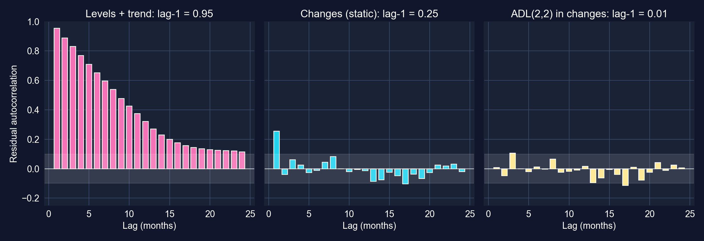
Residual autocorrelations, lags 1–24, for three specifications. Shaded band: ±1.96/√T.

Levels: 0.95. Static changes: 0.25. ADL(2,2): 0.01. Modelling the dynamics leaves residuals that look like white noise.

Left to right, the specifications climb from a spurious-looking levels fit to a well-specified dynamic model. A few isolated bars still touch the band at long lags; with 24 lags, one or two crossings are expected by chance at the 5% level.

Code: compare static, AR(2) and ADL(2,2) on one sample

# continues from the previous block (computed for these slides)
samp = data_rates.dropna(subset=["dgs10_lag2", "dgs1_lag2"])    # same 394 months for all
models = {"static": "dgs10 ~ dgs1", "AR(2)": "dgs10 ~ dgs10_lag1 + dgs10_lag2",
          "ADL(2,2)": "dgs10 ~ dgs10_lag1 + dgs10_lag2 + dgs1 + dgs1_lag1 + dgs1_lag2"}
for name, fml in models.items():
    f = pf.feols(fml, data=samp); n, k = f._N, len(f.coef())
    bic = n * np.log((f._u_hat ** 2).sum() / n) + k * np.log(n)   # lower is better
    print(name, round(f._r2, 3), round(acf(pd.Series(f._u_hat), nlags=1)[1], 3), round(bic, 1))

↗ Try it in Colab

Computed for these slides: the three models are re-fitted on the same 394 months so that R², residual autocorrelation and BIC are comparable.

Output: the ADL wins on every criterion

Model	\(R^2\)	Residual lag-1 \(\rho\)	BIC
Static: \(\Delta\)gs10 on \(\Delta\)gs1	0.573	0.259	−1346.8
AR(2): own lags only	0.125	0.012	−1057.9
ADL(2,2)	0.611	0.008	−1359.7

The chapter’s comparison table (0.57 / 0.25, 0.13 / 0.01, 0.61 / 0.01, with BIC “Higher/Lower”) is confirmed; the BIC values are computed here on a common sample of 394 months so that they are comparable. Note what each part buys: own lags alone explain little (R² 0.125) but whiten the residuals; the short rate explains most of the variation; together, the ADL wins on every criterion. The ADL’s R² gain over the static model is modest (0.038).

Reading time-series regressions with care

• Units: changes are in percentage points, not percent. “A 1% rise in the 1-year rate” should read “a 1-percentage-point rise”
• Levels vs changes answer different questions: equilibrium co-movement vs monthly pass-through
• Stability: one set of coefficients spans 1982–2015, including the zero-lower-bound years after 2008
• Not causal by default: both rates respond to the same news (inflation, growth); the ADL describes predictive dynamics and transmission, not a controlled experiment

A time-series regression is credible when its residuals are white noise and its story survives a check of stability and common shocks.

The chapter’s adjustment example traces the full ADL(2,2) in percentage points: +0.74 on impact, about −0.05 the next month and −0.04 the month after, settling about 0.65 points higher. Cointegration and unit-root tests are the formal tools for the levels question (named in the chapter’s Next Steps), not used here.

Act II-c · From association to cause

17.7 · endogeneity · instrumental variables · the causal toolkit

Section 17.7 is conceptual in the chapter: formulas, a list of methods, and print statements, with no estimation. The deck reviews the concepts and then points to the Chapter 13 deck, where an RCT, a difference-in-differences, a regression discontinuity and an instrumental-variables design are each estimated on real data.

17.7 · When is a slope causal?

Concepts only · worked designs in the Chapter 13 deck

Bridge from the panel and time-series sections: FE removed time-invariant confounders and differencing removed trends, but neither guarantees that the remaining variation in x is as good as random.

OLS is biased the moment \(x\) is correlated with the error

\[y = \beta_1 + \beta_2 x + u, \qquad \text{OLS is consistent only if } E[u \mid x] = 0\]

• Omitted variables: a confounder drives both \(x\) and \(y\). NBA: market size raises revenue and buys wins (FE removed the time-invariant part)
• Measurement error in \(x\): attenuates the slope toward zero
• Simultaneity / reverse causation: \(y\) also moves \(x\). NBA: revenue pays for players, players produce wins

Adding controls fixes only the confounders you measure. Credible causal claims need an identification strategy.

Each source has a different direction of bias. Omitted variables can go either way (sign of the OVB formula); classical measurement error biases toward zero; simultaneity depends on the feedback. Fixed effects address only one specific form of omitted variable: the time-invariant one.

Potential outcomes: what a causal effect means

\[\text{individual effect} = Y_{1i} - Y_{0i}, \qquad \text{ATE} = E[Y_{1i} - Y_{0i}]\]

• \(Y_{1i}\): the outcome if treated; \(Y_{0i}\): the outcome if not. Only one is ever observed
• A naive comparison of treated and untreated: \(E[Y_1\mid D{=}1] - E[Y_0\mid D{=}0] = \text{ATT} + \underbrace{E[Y_0\mid D{=}1]-E[Y_0\mid D{=}0]}_{\text{selection bias}}\)
• Every design is a way to make the selection-bias term zero, or to remove it

A causal estimate is a claim about a counterfactual. The design is the argument for why your comparison group stands in for it.

The chapter defines potential outcomes and the ATE; the decomposition into ATT plus selection bias is the standard result (added as method review, and worked through with data in the Chapter 13 deck’s Act II-b).

Instrumental variables: borrow variation that is as good as random

An instrument \(z\) must satisfy two conditions:

• Relevance: \(\text{Cov}(z, x) \neq 0\). Testable: first-stage \(F\) (rule of thumb \(> 10\))
• Exogeneity / exclusion: \(\text{Cov}(z, u) = 0\), so \(z\) affects \(y\) only through \(x\). Not testable: must be argued

With one regressor and one instrument, substitute \(y = \beta_1 + \beta_2 x + u\) into \(\text{Cov}(z, y)\):

\[\text{Cov}(z,y) = \beta_2\,\text{Cov}(z,x) + \underbrace{\text{Cov}(z,u)}_{=\,0} \;\;\Longrightarrow\;\; \hat\beta_{IV} = \frac{\widehat{\text{Cov}}(z,y)}{\widehat{\text{Cov}}(z,x)} = \frac{\text{reduced form}}{\text{first stage}}\]

IV is consistent where OLS is not, but only for the variation the instrument moves (a local effect), and only as good as the exclusion argument.

The derivation shows exactly where each condition enters: exogeneity kills the Cov(z,u) term; relevance makes the denominator non-zero. A weak first stage (small Cov(z,x)) magnifies any small violation of exogeneity. In pyfixest the syntax is pf.feols(“y ~ 1 | x ~ z”, data=…); a worked example with data is in the Chapter 13 deck (case 13.8).

The causal toolkit

Method	Source of variation	Identifying assumption	Where to see it worked
Randomized experiment	random assignment	randomization intact (no attrition bias)	Ch 13.5 · RAND HIE
Fixed effects	within-unit changes	no time-varying confounders	this deck, 17.3, CS 1, CS 2
Difference-in-differences	group × period	parallel trends	Ch 13.6 · South Africa
Regression discontinuity	a cutoff in a running variable	continuity at the cutoff	Ch 13.7 · U.S. Senate
Instrumental variables	an instrument	relevance + exclusion	Ch 13.8 · institutions
Matching / propensity scores	observed covariates	selection on observables only	(named in the chapter; not worked)

Every row trades the unverifiable “I controlled for everything” for a specific assumption you can defend, probe, or attack.

Links open the Chapter 13 deck at the corresponding case. Fixed effects belong in this table: they are a design, not just an estimator. Their assumption (no time-varying confounders) is weaker than “no confounders” but still an assumption.

The worked designs: naive vs design, from the Chapter 13 deck

Ch 13 case	Design	Naive comparison	Design-based estimate
13.5	RCT (health insurance)	(randomized: no naive version needed)	95% plan: −$1,108 vs free care
13.6	DiD (child nutrition)	treated before vs after: +0.867	+0.522 z-units
13.7	RD (Senate incumbency)	winners vs losers: +21.7 pp	+4.8 pp
13.8	IV (institutions)	OLS: 0.52	2SLS: 0.94

Same lesson as pooled vs FE in this chapter: when the comparison changes, the number changes, sometimes by a factor of four.

Numbers quoted from the verified Chapter 13 deck (see its synthesis act); nothing is re-estimated here. Pair them with this chapter’s own contrasts: NBA pooled 0.0068 vs FE 0.0045; capital elasticity pooled 0.71 vs FE 0.44; population slope pooled +0.34 vs FE −0.82.

Practical recommendations from 17.7

• Name the confounders before running anything; ask which are time-invariant
• Cluster (panels) or use HAC (time series): honest SEs are part of a credible claim
• Report several specifications: pooled and FE, OLS and IV, levels and changes. The pattern of changes is evidence
• State the identifying assumption in one sentence, and say what would violate it

A design earns a causal claim; a significant \(t\)-statistic does not.

These are the chapter’s practical recommendations, with the deck’s thread added: the comparison across specifications is not a robustness ritual, it is the main diagnostic.

Act II-d · Two case studies, every task run

Case Study 1 · cross-country productivity · Case Study 2 · night lights in Bolivia

The chapter’s two end-of-chapter case studies are written as student tasks: Case Study 1 gives hints only; Case Study 2 gives commented-out code. For these slides every task was coded within the chapter’s methods and hints, run, and interpreted. Results that do not appear in the chapter are labelled “computed for these slides”.

Case Study 1 · Does capital raise productivity, within countries?

108 countries × 25 years · variance decomposition · cluster SEs · FE · two-way FE · regions

Mendez (2020) convergence-clubs data. Research question from the chapter: how do physical and human capital relate to labor productivity across countries, and does controlling for unobserved country characteristics change the estimates?

The question and the data

Data. Mendez (2020) convergence-clubs panel: 108 countries × 1990–2014 = 2,700 country-years (balanced).

Variable	Meaning	Mean	Range
ln_lp	log labor productivity (output per worker)	9.80	6.90 – 11.94
ln_kl	log physical capital per worker	10.76	6.59 – 13.22
h	human capital index (schooling-based)	2.99	1.32 – 5.20
region	Africa 26 · Americas 22 · Asia 28 · Europe 30 · Oceania 2 countries

\[\ln lp_{it} = \alpha_i + \beta_k \ln kl_{it} + \beta_h\, h_{it} + \varepsilon_{it}\]

The capital and human-capital columns are kl (capital per worker) and h (human-capital index); the chapter and the slides use them throughout.

Same file as the Mendez case studies of earlier chapters, where kl and h are used correctly. With logs on both sides, beta_k is an elasticity; h enters in levels, so beta_h is a semi-elasticity.

Task 1 · Code: panel structure and variance decomposition

!pip install -q pyfixest                         # pyfixest is not preinstalled in Colab
import numpy as np, pandas as pd, pyfixest as pf # numerics, tables, regressions
base = "https://raw.githubusercontent.com/quarcs-lab/mendez2020-convergence-clubs-code-data/"
dat = pd.read_csv(base + "master/assets/dat.csv")    # 108 countries × 1990–2014
dat["ln_lp"] = np.log(dat["lp"])                     # log labor productivity
dat["ln_kl"] = np.log(dat["kl"])                     # log capital per worker
print(dat["country"].nunique(), dat["year"].nunique(), len(dat))   # 108 25 2700
overall_var = dat["ln_lp"].var()                                    # all country-years
between_var = dat.groupby("country")["ln_lp"].mean().var()          # 108 country means
within_var = dat.groupby("country")["ln_lp"].apply(lambda x: x - x.mean()).var()
print(overall_var, between_var, within_var, between_var / overall_var)

↗ Try it in Colab

Self-contained, and identical to the chapter’s Task 1 code except for the corrected column name. Variances rather than SDs, as in the chapter’s task.

Task 1 · Output: 95% of the variation is between countries

	Variance of ln_lp	Share
Overall (2,700 country-years)	1.391	100%
Between (108 country means)	1.328	95.4%
Within (deviations from own mean)	0.075	5.4%

Shares need not sum to exactly 100%: the between variance is computed over 108 means, the within variance over 2,700 deviations.

Productivity differences are overwhelmingly permanent cross-country gaps. Pooled OLS will be driven by them; fixed effects will keep only the 5% that moves within countries.

Answer to the task’s question: the between component dominates far more than in the NBA (81%). Implication: pooled OLS and FE answer very different questions. Pooled: are capital-rich countries more productive? FE: when a country accumulates capital, does its productivity rise?

Task 2 · Code: pooled OLS with default, robust and cluster SEs

# continues from the previous block
fit_default = pf.feols("ln_lp ~ ln_kl + h", data=dat)                          # iid SEs
fit_hc1 = pf.feols("ln_lp ~ ln_kl + h", data=dat, vcov="HC1")                  # robust
fit_cluster = pf.feols("ln_lp ~ ln_kl + h", data=dat, vcov={"CRV1": "country"})  # by country
print(pd.DataFrame({"default": fit_default.se(), "HC1": fit_hc1.se(),
                    "cluster": fit_cluster.se()}).round(4))   # same coefficients, three SEs
print((fit_cluster.se() / fit_default.se()).round(2))         # inflation factor
fit_cluster.summary()

↗ Try it in Colab

The chapter’s Task 2 code, with ln_kl and h. HC1 is added so the comparison separates heteroskedasticity from within-country dependence.

Task 2 · Output: clustering quadruples the standard errors

Variable	Coef.	Default SE	HC1 SE	Cluster SE	Cluster ÷ default	\(t\) (default → cluster)
Intercept	1.6949	0.0581	0.0724	0.2716	4.67	29.15 → 6.24
ln_kl	0.7136	0.0081	0.0089	0.0327	4.03	87.74 → 21.79
h	0.1410	0.0148	0.0150	0.0612	4.12	9.50 → 2.30

N = 2,700 · 108 country clusters · \(R^2 = 0.908\) · cluster 95% CI: ln_kl [0.6487, 0.7785], h [0.0196, 0.2623] (\(p = 0.023\))

25 years of one country are nearly one observation’s worth of evidence about its level: clustering inflates SEs about 4×. h drops from \(t = 9.5\) to a borderline \(t = 2.3\).

Answer to the task’s question: cluster SEs are about four times the default, much more than the 1.8× in the NBA panel, because country residuals are extremely persistent (95% of variation is between countries, and annual data are smooth). Heteroskedasticity alone (HC1) changes little.

Task 3 · Code: country fixed effects

# continues from the previous block
fit_fe = pf.feols("ln_lp ~ ln_kl + h | country", data=dat,
                  vcov={"CRV1": "country"})          # one intercept per country
fit_fe.summary()                                     # within-country estimates
print(pd.DataFrame({"pooled": fit_cluster.coef(), "FE": fit_fe.coef()}))   # side by side

↗ Try it in Colab

Exactly the chapter’s hint: pf.feols(‘ln_lp ~ ln_kl + h | country’), with SEs clustered by country (computed for these slides; the chapter does not show the output).

Task 3 · Output: capital’s elasticity falls by 39% within countries

Variable	Coef.	SE	\(t\)	\(p\)	95% CI
ln_kl	0.4377	0.0377	11.61	< 0.001	[0.3630, 0.5125]
h	0.2226	0.0566	3.93	< 0.001	[0.1104, 0.3348]

N = 2,700 · 108 country fixed effects · CRV1 by country · within \(R^2 = 0.670\) · computed for these slides

• ln_kl: pooled 0.714 → FE 0.438. Within a country, 1% more capital per worker goes with about 0.44% more output per worker
• h: pooled 0.141 → FE 0.223. One more unit of the index: \(100(e^{0.2226}-1) = 25\%\) higher productivity

The capital slope behaves like the NBA case (a positive confounder removed). Human capital moves the other way: FE does not always shrink coefficients.

Which coefficients change most, and why: the capital elasticity falls by 39%, consistent with positive omitted-variable bias from persistent country traits (institutions, geography, technology levels) that raise both capital per worker and productivity. The human capital coefficient rises, so the time-invariant confounders were correlated with h in the opposite direction relative to productivity, given capital. The chapter’s Key Concept 17.9 says “the typical finding is that FE coefficients are smaller than pooled OLS”; here that holds for capital but not for human capital.

Pooled vs FE vs two-way FE at a glance

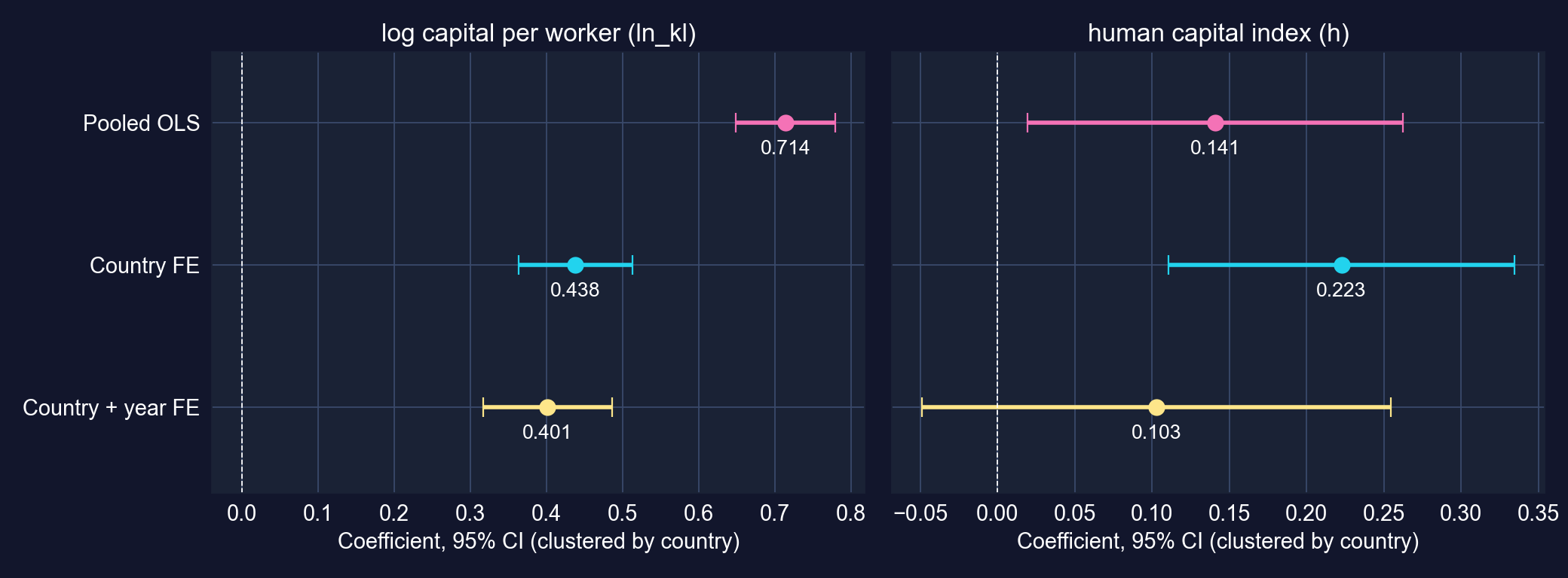
Coefficients with 95% CIs (clustered by country) under three specifications.

Capital’s elasticity is stable once country effects are in (0.44 → 0.40). Human capital’s is not: adding year effects makes it insignificant.

Read across specifications as the thread suggests. ln_kl: 0.714 (pooled), 0.438 (country FE), 0.401 (country and year FE). h: 0.141, 0.223, 0.103 (p = 0.18). The human capital index trends upward almost everywhere, so once common year effects absorb global trends, little independent within-country variation in h is left.

Task 4 · Code: time trends and year effects

# continues from the previous block
fit_twfe = pf.feols("ln_lp ~ ln_kl + h | country + year", data=dat,
                    vcov={"CRV1": "country"})       # two-way FE: country AND year
fit_twfe.summary()
fit_trend = pf.feols("ln_lp ~ ln_kl + h + year | country", data=dat,
                     vcov={"CRV1": "country"})      # a common linear trend instead
fit_trend.summary()
year_fe = fit_twfe.fixef()                          # estimated year effects (1990 = 0)
print(year_fe)

↗ Try it in Colab

The chapter’s hint: pf.feols(‘ln_lp ~ ln_kl + h | country + year’). Year fixed effects absorb everything common to all countries in a given year (global cycles, commodity prices, the 2009 crisis). A linear trend is the restricted version.

Task 4 · Output: common shocks matter for human capital

Variable	Coef.	SE	\(t\)	\(p\)	95% CI
ln_kl	0.4014	0.0428	9.38	< 0.001	[0.3166, 0.4862]
h	0.1028	0.0766	1.34	0.183	[−0.0491, 0.2547]

Two-way FE (country + year) · N = 2,700 · CRV1 by country · within \(R^2 = 0.337\) · computed for these slides

With a linear trend instead of year effects: ln_kl 0.4071, h 0.1009 (\(p = 0.183\)), trend +0.0057 per year (\(p = 0.034\)), i.e. about 0.57% a year of common productivity growth beyond capital and schooling.

Capital’s within-country elasticity survives common shocks (≈ 0.40). Human capital’s does not: its FE estimate partly reflected the worldwide upward trend in schooling.

The within R² falls from 0.670 to 0.337 when year effects are added because the year effects now absorb the common trend that capital and schooling were partly explaining. The trend model and the year-effects model give nearly the same slopes, so the common component is roughly linear.

Task 4 · The common year effects

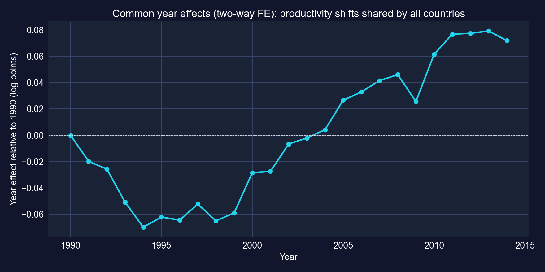
Estimated year fixed effects from the two-way FE model, relative to 1990.

After netting out capital and schooling, the common component falls in the early 1990s, rises from 2000 to 2008, dips in 2009, and recovers.

The 1990s trough (about −0.07 in 1994) partly reflects the transition economies in the sample; the 2009 dip is the global financial crisis. By 2014 the common effect is about +0.07 log points relative to 1990. These are conditional on capital and human capital, so they are a residual “common TFP” path, not total growth.

Task 4 · Code: do regions grow at different rates? Is there convergence?

# continues from the previous block (computed for these slides)
dat["t"] = dat["year"] - 1990                                    # years since 1990
fit_rt = pf.feols("ln_lp ~ ln_kl + h + i(region, t) | country", data=dat, vcov={"CRV1": "country"})
names = fit_rt.coef().index; rt = [k for k in names if k.startswith("region::")]
R = np.zeros((len(rt) - 1, len(names)))                           # H0: all trends = Africa's
for j, k in enumerate(rt[1:]):
    R[j, names.get_loc(k)], R[j, names.get_loc(rt[0])] = 1, -1
print(fit_rt.coef()[rt]); print(fit_rt.wald_test(R=R))           # Wald chi2(4)
first = dat[dat["year"] == 1990].set_index("country")["ln_lp"]   # initial productivity
last = dat[dat["year"] == 2014].set_index("country")["ln_lp"]
conv = pd.DataFrame({"ln_lp0": first, "g": 100 * (last - first) / 24}).reset_index()
pf.feols("g ~ ln_lp0", data=conv, vcov="HC1").summary()          # growth on initial level

↗ Try it in Colab

The task asks to “test whether productivity growth rates differ across regions” and “is there evidence of convergence”. i(region, t) gives each region its own linear trend (region-time interactions, as the hint suggests), with country FE. Convergence: regress average annual growth 1990–2014 on initial log productivity (a simple cross-country regression; growth in % per year uses the log-difference approximation).

Task 4 · Output: regional trends differ; poorer countries did not catch up

Region trend (per year)	Coef.	\(p\)
Africa	0.0015	0.665
Americas	0.0066	0.035
Asia	0.0135	0.010
Europe	0.0126	0.001
Oceania (2 countries)	0.0067	< 0.001

Country FE + ln_kl + h · CRV1 · equal-trends test: Wald \(\chi^2(4) = 11.39\), \(p = 0.023\)

Convergence regression	Coef.	SE	\(p\)
Intercept	4.520	1.836	0.015
ln_lp0 (1990)	−0.222	0.180	0.221

N = 108 · HC1 · \(R^2 = 0.018\) · growth in % per year

Beyond capital and schooling, productivity trended up about 1.3% a year in Asia and Europe and barely at all in Africa. There is no unconditional convergence: the slope on initial productivity is small and insignificant.

Both computed for these slides. Region trends are conditional on capital, human capital and country FE, so they are regional “residual TFP” trends. The convergence slope of −0.22 means a country with 1 log point lower productivity in 1990 grew only 0.22 percentage points a year faster, and that difference is not statistically distinguishable from zero. Average annual growth by region (raw, not conditional): Asia 3.25%, Europe 2.67%, Americas 2.23%, Africa 1.41%, Oceania 1.33%.

Task 4 · Convergence, pictured

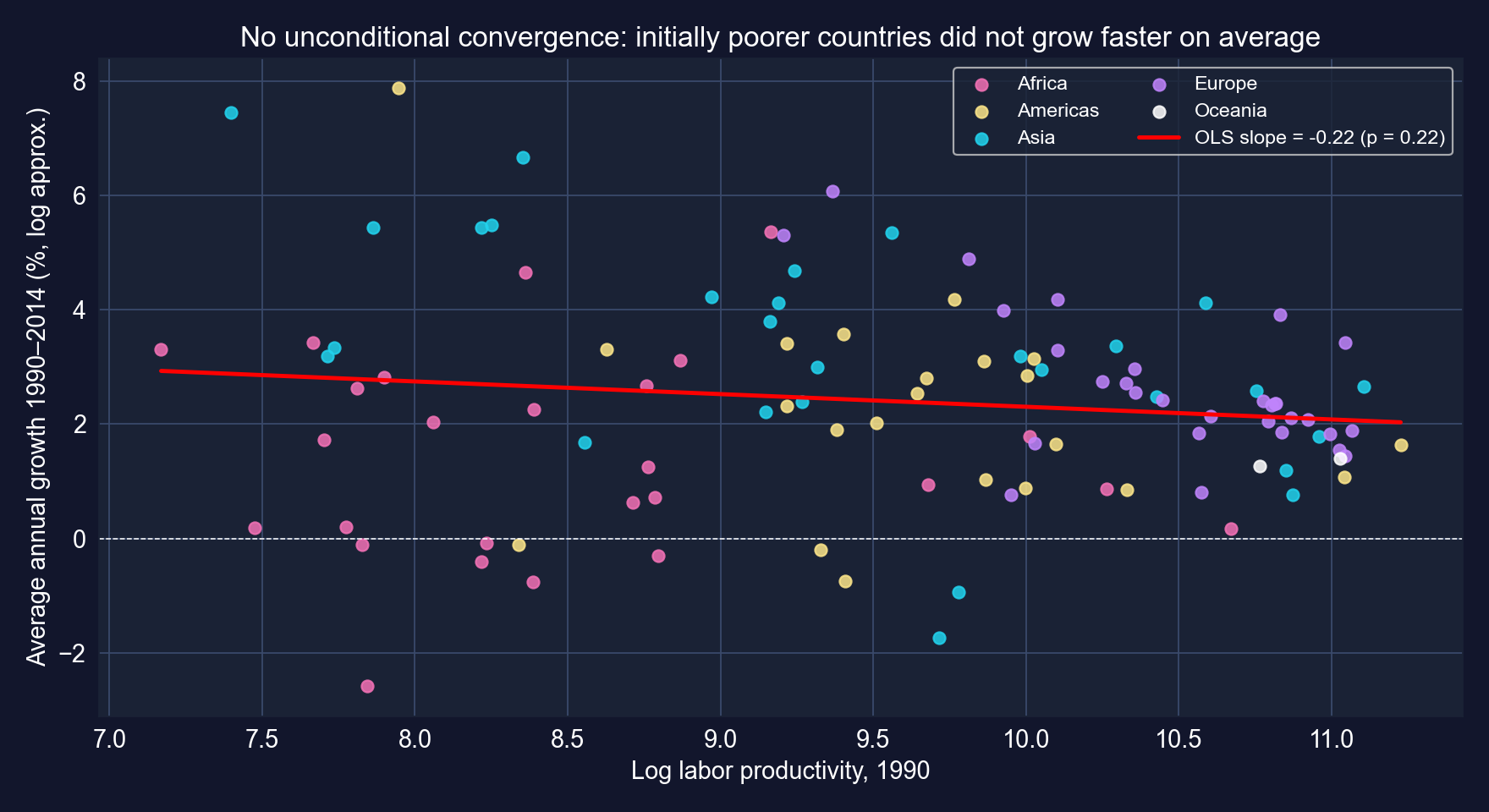
Average annual growth of labor productivity, 1990–2014, against its 1990 level; 108 countries.

A cloud with a faintly negative slope: some poor Asian economies raced ahead, many African economies did not. This is why the Mendez data are about convergence clubs, not one global convergence.

The picture motivates club convergence: groups of countries converge to different steady states. Testing for clubs is beyond this chapter.

Task 5 · Code: do returns to capital differ by region?

# continues from the previous block (computed for these slides)
fit_r1 = pf.feols("ln_lp ~ ln_kl + h + C(region)", data=dat, vcov={"CRV1": "country"})
fit_r2 = pf.feols("ln_lp ~ ln_kl + h + C(region) + C(region):ln_kl + C(region):h",
                  data=dat, vcov={"CRV1": "country"})    # region-specific slopes
fit_r1.summary(); fit_r2.summary()
inter = [k for k in fit_r2.coef().index if ":" in k]     # the 8 interaction terms
R = np.array([[1.0 * (k == a) for k in fit_r2.coef().index] for a in inter])
print(fit_r2.wald_test(R=R))                             # H0: all 8 interactions = 0

↗ Try it in Colab

The task’s three steps: region dummies, region-by-capital interactions, and a joint test. Africa is the reference region (alphabetical first). Pooled specifications with country-clustered SEs, as the task does not ask for FE here.

Task 5 · Output: regional slopes differ only weakly

Region	Implied ln_kl slope	Implied h slope
Africa (reference)	0.640	0.257
Americas	0.671	0.293
Asia	0.778	−0.075
Europe	0.679	0.048
Oceania (2 countries)	0.649	0.110

Implied slope = base slope + region interaction · joint test of all 8 interactions: Wald \(\chi^2(8) = 13.90\), \(p = 0.084\) · region dummies alone: only Oceania differs from Africa (\(p = 0.034\)) · computed for these slides

Returns to capital look similar across regions (0.64–0.78), and the interactions are jointly significant only at 10%. No region-specific interaction is individually significant at 5%.

Which region shows the highest return to human capital? The Americas (0.29) and Africa (0.26), but the h interactions are imprecise (the Asia interaction has p = 0.13), so the ranking is not reliable. These are pooled cross-country associations, subject to all the confounding that Task 3 revealed.

Task 6 · The policy brief, in numbers

Specification	ln_kl	h	Variation used
Pooled OLS, cluster SEs	0.714 (0.033)	0.141 (0.061)	between + within
Country FE	0.438 (0.038)	0.223 (0.057)	within country
Country + year FE	0.401 (0.043)	0.103 (0.077)	within country, net of common shocks
Region-specific slopes (pooled)	0.64 – 0.78	−0.08 – 0.29	between + within, by region

• Channels: capital accumulation is robustly associated with productivity within countries (elasticity ≈ 0.4); the human-capital link is fragile once common trends are removed
• Causal? Not established: capital responds to expected productivity (reverse causality), and time-varying policies and shocks remain

Policy reading: investment climates that raise capital per worker are the best-supported channel in these data, and pooled cross-country estimates overstate it by about 40%.

The task asks for a 200–300 word brief. This slide gives its evidence base. Threats to identification: reverse causality (more productive economies attract investment), measurement error in capital stocks (built by perpetual inventory, which smooths within variation), and the human capital index trending smoothly. The chapter’s Key Concept 17.10 adds that the estimator choice should follow the question; here the within estimates are the relevant ones for “what happens when a country accumulates capital”.

Case Study 2 · Night lights and population in Bolivia

339 municipalities × 2012–2020 · reshaping · pooled · FE · year effects · first differences

DS4Bolivia: the final DS4Bolivia case study of the book. The cross-sectional satellite-development data become a panel because nighttime lights and population are available annually for 2012–2020.

The question and the data

Data. DS4Bolivia (ds4bolivia_v20250523.csv): 339 municipalities, annual columns ln_NTLpc2012 … ln_NTLpc2020 and pop2012 … pop2020, stored wide (one row per municipality).

Variable	Meaning
ln_NTLpc	log nighttime lights per capita (outcome)
ln_pop	log population
year	2012, …, 2020
asdf_id, mun, dep	municipality id, name, department (9 departments)

\[\ln NTLpc_{it} = \alpha_i + \beta\,\ln pop_{it} + \delta_t + \varepsilon_{it}\]

Research question: how does luminosity evolve within municipalities over time, and how does it move with population once fixed local traits (altitude, remoteness, climate) are removed?

Key interpretive point for later: the outcome is lights per capita, ln(NTL) − ln(pop). So the coefficient on ln_pop equals (elasticity of total lights with respect to population) − 1. A coefficient of zero would mean total lights grow one-for-one with population.

Task 1 · Code: reshape wide → long

!pip install -q pyfixest                         # pyfixest is not preinstalled in Colab
import numpy as np, pandas as pd, pyfixest as pf # numerics, tables, regressions
url_bol = "https://raw.githubusercontent.com/quarcs-lab/ds4bolivia/master/ds4bolivia_v20250523.csv"
bol = pd.read_csv(url_bol)                       # 339 municipalities, wide format
years = range(2012, 2021)                        # nine annual observations
ntl_long = bol[["mun", "dep", "asdf_id"] + [f"ln_NTLpc{y}" for y in years]].melt(
    id_vars=["mun", "dep", "asdf_id"], var_name="ntl_var", value_name="ln_NTLpc")
ntl_long["year"] = ntl_long["ntl_var"].str.extract(r"(\d{4})").astype(int)  # "…2015" → 2015
pop_long = bol[["asdf_id"] + [f"pop{y}" for y in years]].melt(
    id_vars=["asdf_id"], var_name="pop_var", value_name="pop")
pop_long["year"] = pop_long["pop_var"].str.extract(r"(\d{4})").astype(int)

↗ Try it in Colab

The chapter’s commented-out Task 1 code, uncommented and run. melt() turns nine NTL columns into nine rows per municipality; the year is extracted from the column name with a regular expression.

Task 1 · Code: merge into one panel and check it

# continues from the previous block
panel = ntl_long.merge(pop_long[["asdf_id", "year", "pop"]], on=["asdf_id", "year"], how="left")
panel["ln_pop"] = np.log(panel["pop"])                       # log population
panel = panel.sort_values(["asdf_id", "year"]).reset_index(drop=True)
print(panel.shape, panel["asdf_id"].nunique())               # rows × columns, municipalities
print(panel["ln_NTLpc"].isna().sum())                        # missing light values
panel_reg = panel[["ln_NTLpc", "ln_pop", "year", "mun", "dep", "asdf_id"]].dropna()
print(len(panel_reg), panel_reg["asdf_id"].nunique())        # estimation sample

↗ Try it in Colab

	Rows	Municipalities
Full panel (339 × 9)	3,051	339
Missing ln_NTLpc	67
Estimation sample	2,984	337

The panel is 339 × 9 = 3,051 as the task expects, but 67 municipality-years have no light value, so the estimation sample is 2,984 rows covering 337 municipalities (two lose all years). The panel is therefore unbalanced; report this.

Task 6 (first): levels differ far more than they move

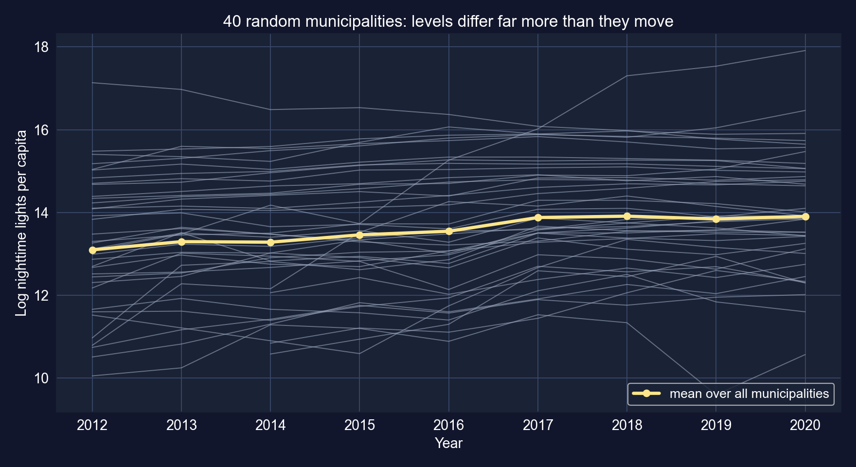
Log night lights per capita for 40 randomly chosen municipalities, with the all-municipality mean.

Variance of…	Overall	Between	Within	Between share
ln_NTLpc	1.729	1.635	0.220	94.6%
ln_pop	1.278	1.283	0.0055	≈ 100% (within 0.4%)

Moved forward from Task 6 because it frames everything that follows (computed for these slides). Lights: 95% between municipalities, like the countries. Population: essentially all between; within-municipality population barely moves (within variance 0.0055, about 0.4% of the total). That will matter for the FE estimate of the population slope: it is identified from very little variation. The between share slightly exceeds 100% for ln_pop because between and within variances use different denominators.

Task 2 · Code: pooled OLS, default vs cluster SEs

# continues from the previous block
fit_def = pf.feols("ln_NTLpc ~ ln_pop + year", data=panel_reg)               # default SEs
fit_pooled = pf.feols("ln_NTLpc ~ ln_pop + year", data=panel_reg, vcov={"CRV1": "asdf_id"})
print((fit_pooled.se() / fit_def.se()).round(2))      # cluster ÷ default, per coefficient
fit_pooled.summary()

↗ Try it in Colab

The chapter’s commented Task 2 code, uncommented: the same pooled regression with default and with municipality-clustered SEs.

Task 2 · Output: population and trend, pooled

Variable	Coef.	SE	\(t\)	\(p\)	95% CI
Intercept	−200.1384	12.3774	−16.17	< 0.001	[−224.4854, −175.7914]
ln_pop	0.3385	0.0472	7.18	< 0.001	[0.2457, 0.4312]
year	0.1044	0.0062	16.88	< 0.001	[0.0923, 0.1166]

N = 2,984 · 337 clusters · \(R^2 = 0.130\) · cluster ÷ default SE: ln_pop 2.37, year 0.71

The chapter’s commented Task 2 code. The intercept is the predicted log lights at year 0 (an extrapolation two thousand years back), which is why it is −200; centre the year to make it interpretable. Clustering widens the population SE 2.37×, but it narrows the SE on year (0.71×). Cluster-robust SEs estimate the actual within-cluster covariance of regressor × residual; when those products are negatively correlated within clusters, the cluster SE is smaller than the default. Cluster SEs are not always larger.

Task 2 · Interpretation: bigger places, more light per person

• Across municipalities, 1% more population goes with 0.34% more light per capita
• In total light, that is an elasticity of \(0.34 + 1 = 1.34\): larger places are disproportionately brighter (towns, grids, commerce)
• Trend: lights per capita grew about 0.10 log points a year on average, holding population fixed
• Low \(R^2 = 0.13\): most of the variation in lights per capita is unrelated to population size

A between-municipality comparison: cities versus rural municipalities differ in far more than population.

The per-capita construction matters: regress ln(NTL/pop) on ln(pop), and the slope is the total-lights elasticity minus one. Altitude, remoteness, grid access and economic structure differ systematically with size. FE next removes the time-invariant part of those differences.

Task 3 · Code: municipality fixed effects

# continues from the previous block
fit_fe = pf.feols("ln_NTLpc ~ ln_pop + year | asdf_id", data=panel_reg,
                  vcov={"CRV1": "asdf_id"})          # within-municipality estimator
fit_fe.summary(); print(fit_pooled.coef()["ln_pop"], fit_fe.coef()["ln_pop"])

↗ Try it in Colab

The chapter’s commented Task 3 code. The vertical bar absorbs one intercept per municipality, which is the same as demeaning every variable by municipality.

Task 3 · Output: the population slope flips sign

Variable	Coef.	SE	\(t\)	\(p\)	95% CI
ln_pop	−0.8237	0.2942	−2.80	0.005	[−1.4023, −0.2450]
year	0.1320	0.0066	20.04	< 0.001	[0.1191, 0.1450]

N = 2,983 (one singleton dropped) · 337 municipality FE · CRV1 · within \(R^2 = 0.429\)

The population slope flips sign: +0.34 pooled, −0.82 within municipalities.

The chapter’s commented Task 3 code (pyfixest absorbs the municipality effects; equivalent to demeaning). N is 2,983 because one municipality has a single observation, which carries no within variation and is dropped. The year coefficient rises to 0.132 log points a year (about 14% a year in per-capita lights).

Task 3 · Interpretation: what the sign flip does and does not mean

• In total lights: \(-0.82 + 1 = 0.18\). When a municipality’s population grows faster than its own trend, its total light grows much less than proportionally, so light per person falls
• Fixed effects absorb altitude, remoteness, climate, historical infrastructure: the cross-sectional “size premium” was mostly these traits
• But within-municipality population varies very little (0.4% of its variance) and moves almost linearly with time. With a year trend in the model, \(\beta\) is identified from small deviations of population from its trend

Treat −0.82 as fragile: population figures between censuses are usually projections, so their year-to-year deviations may be smoothing artefacts, not real migration.

Within municipalities the demeaned log population and demeaned year correlate 0.59 (computed for these slides), so the trend absorbs much of the population variation. The census-projection caveat is a standard data-quality concern for intercensal population series; the dataset documentation should be checked before reading the coefficient as behavioural.

Task 4 · Code: year effects instead of a linear trend

# continues from the previous block
fit_yfe = pf.feols("ln_NTLpc ~ ln_pop + C(year) | asdf_id", data=panel_reg,
                   vcov={"CRV1": "asdf_id"})                 # 2012 = reference year
yk = [k for k in fit_yfe.coef().index if k.startswith("C(year)")]
R = np.array([[1.0 * (k == a) for k in fit_yfe.coef().index] for a in yk])
print(fit_yfe.wald_test(R=R))                                # H0: no year effects
print(fit_yfe.coef()[yk].round(3))                           # path relative to 2012

↗ Try it in Colab

The task: replace the linear trend with year dummies, test their joint significance, and plot them. Municipality FE stay in, so the year effects describe the average within-municipality path, holding population fixed. (The chapter’s example code plots raw yearly means; the regression version is used here, and the raw means tell the same story: 13.10 in 2012, 13.91 in 2020.)

Task 4 · Output: lights jump in 2017, then plateau

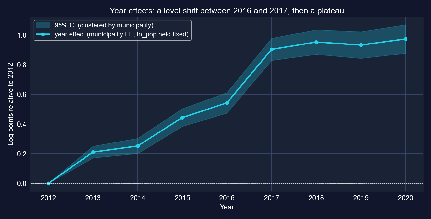
Year effects (log points relative to 2012), with municipality FE and log population held fixed.

Joint test of the 8 year effects: Wald \(\chi^2(8) = 706.3\), \(p < 0.001\) · ln_pop −0.8173 (SE 0.2957) · within \(R^2 = 0.469\) · computed for these slides

Not steady growth: +0.54 by 2016, a jump of 0.36 to 2017, then a plateau near +0.95. Ask whether the satellite product or its processing changed before reading a jump as development.

Year effects: 2013 0.211, 2014 0.252, 2015 0.444, 2016 0.543, 2017 0.904, 2018 0.953, 2019 0.933, 2020 0.974. The linear trend of 0.132 per year in Task 3 averaged over this step-plus-plateau shape. Annual nighttime-lights composites can change with sensor calibration and processing; this is a caution to check the data documentation, not a claim about what happened in 2017. The population coefficient is unchanged by the switch from trend to dummies.

Task 5 · Code: first differences

# continues from the previous block
panel_reg = panel_reg.sort_values(["asdf_id", "year"])
panel_reg["d_ln_NTLpc"] = panel_reg.groupby("asdf_id")["ln_NTLpc"].diff()   # vs previous row
panel_reg["d_ln_pop"] = panel_reg.groupby("asdf_id")["ln_pop"].diff()
fd_data = panel_reg.dropna(subset=["d_ln_NTLpc", "d_ln_pop"])               # drop first years
fit_fd = pf.feols("d_ln_NTLpc ~ d_ln_pop", data=fd_data, vcov={"CRV1": "asdf_id"})
fit_fd.summary()                                                            # change on change

↗ Try it in Colab

Sort by municipality and year, take within-municipality differences, drop each municipality’s first year, and regress change on change with municipality-clustered SEs.

Task 5 · Output: first differences point the same way, less precisely

Variable	Coef.	SE	\(t\)	\(p\)	95% CI
Intercept	0.1200	0.0059	20.29	< 0.001	[0.1083, 0.1316]
d_ln_pop	−0.5205	0.2928	−1.78	0.076	[−1.0964, 0.0554]

N = 2,647 · CRV1 by municipality · \(R^2 = 0.002\) · the intercept is the average yearly change (≈ +12.7% a year in per-capita lights)

The chapter’s commented Task 5 code. diff() takes the change from the previous available row; where a year is missing it spans two years (a small number of cases). The intercept in a first-difference regression plays the role of the linear trend.

Task 5 · The population slope across four estimators

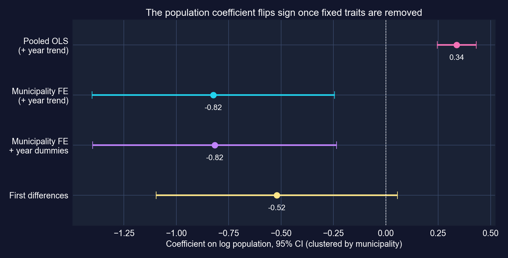
Coefficient on log population, 95% CIs clustered by municipality, across four specifications.

Positive between municipalities, negative within them, and only borderline in first differences.

Pooled +0.34; FE with a trend −0.82; FE with year dummies −0.82; FD −0.52. Only the pooled estimate uses between-municipality variation.

Task 5 · FE vs FD: same idea, different weights

• Both remove \(\alpha_i\). FE compares each year with the municipality’s 9-year average; FD compares each year with the previous one
• With \(T > 2\) they differ when errors are serially correlated or the timing of effects matters: FE is efficient with serially uncorrelated errors, FD with random-walk errors
• Here: FE −0.82 (\(p = 0.005\)), FD −0.52 (\(p = 0.076\)); same sign, overlapping CIs

Both point the same way, but FD cannot reject zero at 5%. The population slope is the weakest link in this case study.

Total-lights elasticities implied: pooled 1.34, FE 0.18, FD 0.48. When FE and FD diverge, it often signals measurement error (differencing amplifies noise relative to signal) or dynamics; both apply here, given how little population moves within municipalities.

Task 6 · Code: the evidence for the panel brief

# continues from the previous block (computed for these slides)
for v in ["ln_NTLpc", "ln_pop"]:
    overall = panel_reg[v].var()                                       # all rows
    between = panel_reg.groupby("asdf_id")[v].mean().var()            # municipality means
    within = panel_reg.groupby("asdf_id")[v].apply(lambda x: x - x.mean()).var()
    print(v, round(overall, 4), round(between, 4), round(within, 4))
dep = panel_reg.pivot_table(index="dep", columns="year", values="ln_NTLpc", aggfunc="mean")
print((dep[2020] - dep[2012]).sort_values().round(2))                 # change by department

↗ Try it in Colab

The task’s suggested extras: variance decomposition (shown earlier) and growth by department. Mean change in log lights per capita, 2012–2020, over all municipalities: +0.81.

Task 6 · The panel brief, in numbers

Evidence	Result
Variation in ln_NTLpc	95% between municipalities; within changes are small but real
Pooled population slope	+0.34 (cluster SE 0.047): bigger places brighter per person
FE / FD population slope	−0.82 (\(p = 0.005\)) / −0.52 (\(p = 0.076\)): fragile
Time path (year effects)	+0.97 log points 2012 → 2020, with a 0.36 jump in 2017
By department, 2012 → 2020	Chuquisaca +1.24, Beni +1.20, La Paz +1.04 … Tarija +0.46, Pando −0.50

• Advantages: annual, consistent coverage of all municipalities where surveys are rare
• Limits: sensor changes; a projected population denominator; lights see electrified activity only
• Add: time-varying covariates (electrification, roads, transfers)

Satellite panels can track municipal change over time, but the within-municipality slope is only as good as the time variation in the regressor.

Answers to the brief’s questions: (1) within-municipality changes show broad brightening, front-loaded into 2017; (2) the FE population coefficient reverses the pooled sign; (3) the time trend is step-shaped, not linear; (4) FE and FD agree in sign, differ in size and precision; the key assumptions are no time-varying confounders (both) and the error structure (which is more efficient); (5) and (6) as on the slide. Pando is the only department whose mean per-capita lights fell.

Reading it right

Act III · The resolution

Synthesis: line up every coefficient by the variation that identified it, line up every standard error by the dependence it allowed, then leave with a decision guide and a checklist.

Which variation identified each slope?

Example	Coefficient	All variation (pooled / levels)	Within or changes only	Change
NBA revenue	wins	0.00675	FE: 0.00451	−33%
Productivity, 108 countries	ln_kl	0.714	FE: 0.438	−39%
Productivity, 108 countries	h	0.141	FE: 0.223	+58%
Night lights, 337 municipalities	ln_pop	+0.338	FE: −0.824; FD: −0.521	sign flips
Treasury rates	1-year rate	levels + trend: 0.508	changes: 0.720	different question

No rule says the within estimate is smaller. It can shrink, grow or flip. What is constant is the lesson: the comparison defines the coefficient.

The deck’s thread in one table. In the panels, the move from pooled to within removes time-invariant confounders; the direction of the change depends on how those confounders relate to x and y. In the time series, levels and changes estimate different objects (an equilibrium co-movement net of a linear trend versus monthly pass-through), so the comparison is not about bias alone.

Which standard error was honest?

Example	Honest SE	Ratio to default SE	What the default ignored
NBA, pooled	cluster by team	1.81	10 seasons of one team are correlated
NBA, FE	cluster by team	1.42	serial correlation left after removing \(\alpha_i\)
Countries, pooled	cluster by country	4.03 (ln_kl)	25 smooth years per country
Municipalities, pooled	cluster by municipality	2.37 (ln_pop), 0.71 (year)	within-municipality dependence, either sign
Treasury rates, levels	Newey–West, 24 lags	3.65	residual autocorrelation of 0.95

Same coefficients, very different confidence. Inference must allow the dependence the data actually have, and it can move the SE either way.

Every ratio is computed from the same regressions shown in the deck. The 0.71 for the municipal year trend is the reminder that clustering is not a fixed “inflate by k” adjustment: it estimates the actual within-cluster covariance.

Choosing an estimator: a short guide

• Unit traits drive both \(x\) and \(y\)? Fixed effects (plus time effects); cluster by unit
• Unit effects unrelated to \(x\)? Random effects; check with Hausman or Mundlak
• Trending time series? Check the correlogram; use changes or AR/ADL dynamics; HAC SEs
• Binary outcome? LPM for averages; logit for probabilities, with marginal effects
• Time-varying confounders or feedback? You need a design: IV, DiD, RD, RCT

Start from the structure of the data and the likely confounders, then pick the estimator, then the standard error.

A decision guide, not an algorithm. Many applied papers combine elements: two-way FE with clustered SEs is the default panel specification in much of applied economics, and DiD is two-way FE with a treatment indicator.

The tempting mistake — and the correction

Objection. “Fixed effects control for unobserved heterogeneity, so the FE coefficient is causal.”

Response. FE remove only what is constant within a unit. In the NBA a new star raises wins and revenue in the same season; in Bolivia population and lights co-move with whatever drives local growth. And FE throw away the between variation, so the estimate rests on the within variation that remains: 69% of the variance of wins, but only 0.4% of the variance of municipal population.

FE are a design with an assumption (no time-varying confounders) and a cost (less variation). Check both before saying “effect”.

Steelman the objection: FE do solve a large class of omitted-variable problems, and the move from pooled to FE is often the single most informative robustness check in a panel. But “unobserved heterogeneity” in the FE sense means time-invariant heterogeneity only.

Five questions to ask of any panel or time-series coefficient

1. Which variation? Between, within, changes, or two shared trends?
2. Which units? Log points, percent, percentage points, probability, odds?
3. Which standard error? Clustered at the level where shocks are shared, or HAC over the right horizon?
4. What is held fixed? Unit effects, time effects, a trend, lagged values?
5. What could still move both \(x\) and \(y\)? Time-varying confounders, feedback, common shocks?

The unit errors corrected in this deck: rate changes in percentage points (not %), logit coefficients as log-odds (not probabilities), and log-point effects converted with \(e^b - 1\).

A checklist students can apply to any output in this chapter. The unit conventions to watch: “1%” versus a one-percentage-point rate change, marginal effects labelled as average versus at-the-means, and exact percentage conversions for log-level coefficients.

What to carry forward

• Panels: decompose the variation; FE use only the within part; cluster by unit
• FE vs RE: FE survive correlated unit effects; RE needs them uncorrelated
• Logit: report marginal effects, and say AME or MEM
• Time series: high \(R^2\) in levels is a warning; check residual autocorrelation
• Dynamics: ADL multipliers trace how effects build (0.74 → 0.53)
• Causation: FE and differencing remove some confounders; designs handle the rest

Recap of the chapter’s Key Takeaways, updated with what the deck verified: the size of the clustering and HAC corrections, the pooled-to-FE changes in three panels, and the ADL dynamics.

Structure, memory and a credible design: that is what turns a slope into an answer.