Summary

Chapter 3 — The neoclassical growth model

At a glance. The Solow model fixed the saving rate. This chapter lets households choose how much to save, trading consumption today against consumption tomorrow. The result is the Ramsey–Cass–Koopmans model: the first dynamic general equilibrium model of the book, and the source of its most important equation.

Thesis. When households choose saving optimally, consumption grows exactly when the return on capital exceeds their impatience, and the economy glides along a unique saddle path to a steady state with no oversaving. Yet, as in Solow, income per person still does not grow in the long run.

Before you start

This chapter builds on the Solow model (book, Chapter 2): steady states, the golden rule, per-capita variables. It also uses three tools from the book’s mathematical appendix, each explained along the way: the current-value Hamiltonian for dynamic optimisation, phase diagrams for two-variable systems, and eigenvalues of a 2×2 matrix. You also need to be comfortable with growth rates (\(\dot x / x\)) and elasticities.

Readiness check — three quick questions

In the Solow model, what condition pins down the steady-state capital stock?
What does the golden rule maximise?
A 2×2 matrix has a negative determinant. What do you know about the signs of its eigenvalues?

Answers.

Saving equals break-even investment, \(s f(k^*) = (n+\delta)k^*\).
Steady-state consumption per capita.
They have opposite signs, because the determinant is their product.

Missed one? Review Chapter 2 for 1–2 and the book’s mathematical appendix for 3.

Learning objectives

After this chapter you can:

explain the trade-off behind the Euler equation and predict the direction of consumption growth;
find the steady state from the \(\dot k = 0\) and \(\dot c = 0\) loci and explain why it lies below the golden rule (the modified golden rule);
predict how consumption and capital respond, on impact and over time, to a permanent change in patience;
🔵 read a phase diagram and explain why only the saddle path is an equilibrium;
🔵 evaluate Piketty’s \(r > g\) argument within the model;
🔴 derive the Euler equation from the Hamiltonian and prove saddle-path stability;
🔴 show that the decentralised equilibrium reproduces the planner’s solution.

Visual roadmap

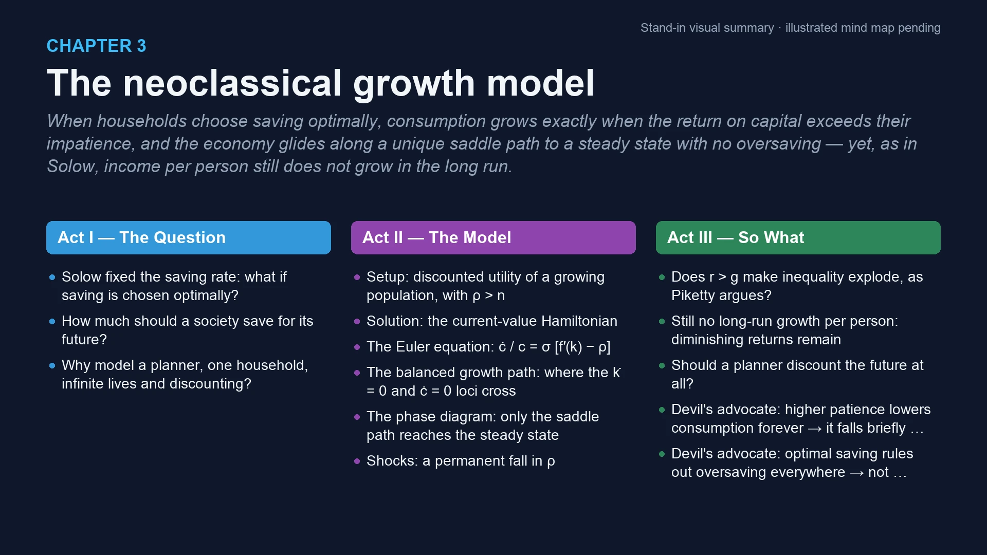
Visual summary of Chapter 3: the question, the model and the so-what of the neoclassical growth model — The chapter at a glance: its three acts (the question, the model, so what)

Section-by-section summary

3.1 The Ramsey problem

The chapter replaces Solow’s constant saving rate with an optimal saving plan. A planner chooses consumption over time to maximise the discounted welfare of a representative household.
Frank Ramsey solved the problem in 1928. Cass and Koopmans revived it in the 1960s, hence the names Ramsey or Ramsey–Cass–Koopmans model, or neoclassical growth model (NGM).
The shortcuts are bold but defensible:
- The planner reproduces the competitive outcome under the welfare theorems.
- One household is fine if people respond similarly to incentives.
- Infinite lives stand in for families that care about their children.
- Discounting reflects the revealed preference behind positive interest rates.
- 🔵 Barro’s dynastic altruism turns finite lives into an infinite horizon. Caselli and Ventura show that structured heterogeneity is still compatible with a representative household.
Why it matters: this is the template of modern macroeconomics. Explicit preferences make welfare statements possible, which the Solow model could not support.

The consumer’s problem

The household maximises discounted utility summed over all its members: \[\int_0^\infty u(c_t)\, e^{nt} e^{-\rho t}\, dt\] In words: utility of per-capita consumption, counted for a population growing at rate \(n\) and discounted at the rate of time preference \(\rho\).
Utility is increasing and concave (\(u' > 0\), \(u'' \le 0\)) and satisfies the Inada conditions.
🔵 The model needs \(\rho > n\). Otherwise future generations’ larger numbers outweigh discounting, and the household would postpone consumption forever, so the problem has no solution.
Why it matters: \(\rho\) is the single number that encodes impatience. Almost every result below compares something with \(\rho\).
Practise it: Quiz 1

The resource constraint

With no depreciation and no government, output is either consumed or invested: \(\dot K = F(K, L) - C\).
In per-capita terms (using constant returns, and \(\dot K/L = \dot k + nk\)): \[\dot k_t = f(k_t) - n k_t - c_t\] In words: capital per person grows by what output leaves after consumption and after equipping the newcomers (“capital widening”, \(nk\)).
This equation of motion makes the problem dynamic: saving today sets the capital available tomorrow.
Capital is the state variable: sticky, it can only change gradually. Consumption is the control variable: jumpy, it can be chosen freely at any instant.
Why it matters: the sticky/jumpy distinction decides how the economy reacts to shocks. Consumption absorbs the surprise; capital follows.
Practise it: Quiz 5

Solution to consumer’s problem

🔵 The tool is the current-value Hamiltonian, \(H = u(c)e^{nt} + \lambda[f(k) - nk - c]\). The co-state \(\lambda_t\) is the shadow value of a unit of capital at time \(t\).
🔵 The first-order conditions are:
- static: \(u'(c)e^{nt} = \lambda\), so the marginal utility of consuming equals the value of saving;
- dynamic: \(\dot\lambda = -\lambda[f'(k) - n] + \rho\lambda\);
- transversality (TVC): \(\lim_{t\to\infty} k_t \lambda_t e^{-\rho t} = 0\).
🔵 The dynamic condition is an arbitrage equation for capital as an asset, \(\rho + n = \dot\lambda/\lambda + f'(k)\): the opportunity cost of holding capital equals its dividend plus its capital gain.
🔴 The TVC says the optimiser never “dies” holding valuable capital that could have been consumed.
Why it matters: “return = opportunity cost” is the arbitrage logic the book reuses for investment, asset prices and policy.
Practise it: Exercise 6 · Quiz 8 · 🔴 Proof

The balanced growth path and the Euler equation

Differentiating the static condition in time, and defining the elasticity of intertemporal substitution \(\sigma \equiv -u'(c)/(u''(c)c) > 0\), gives the Euler equation (Keynes–Ramsey rule): \[\frac{\dot c_t}{c_t} = \sigma\,[f'(k_t) - \rho]\] In words: consumption grows when saving’s return \(f'(k)\) beats impatience \(\rho\), and faster the more willing households are to shift consumption over time (\(\sigma\)).
The Euler equation and the resource constraint form a system of two differential equations in \((c, k)\). Together with \(k_0\) and the TVC, they determine the whole path.
\(\dot k = 0\) gives \(c = f(k) - nk\), a hump. Above it capital falls; below it capital rises.
\(\dot c = 0\) gives \(f'(k^*) = \rho\), a vertical line. To its left consumption rises; to its right it falls.
The steady state is where the two cross. Comparing it with the golden rule \(f'(k_G) = n\) yields the modified golden rule: \[f'(k^*) = \rho > n = f'(k_G) \;\Rightarrow\; k^* < k_G\] In words: optimal saving stops short of the capital stock that maximises steady-state consumption, because the sacrifices needed to get there are discounted.
🔵 The Solow model allows dynamic inefficiency (oversaving), but optimal saving rules it out. Whether oversaving can happen in practice returns in Chapter 8.
Why it matters: the Euler equation “may well be the most important equation in all of macroeconomics”: every intertemporal choice in the book is a variation on it.
Practise it: Worked example · Exercises 1–2 · Key graph: the Euler equation · Key graph: the golden rule · Quiz 4

A digression on inequality: Is Piketty right?

On the balanced growth path output grows at \(g = n\). In the market economy \(r = f'(k^*) = \rho > n\), so the model’s dynamic efficiency is exactly Piketty’s \(r > g\), his “fundamental force for divergence”.
Piketty’s worry is that, if \(r > g\), inherited wealth grows faster than income and inequality explodes.
The chapter’s caveats:
- what \(k\) measures (much of it may be human capital, earned by labour);
- social mobility between workers and capitalists (Acemoglu and Robinson);
- how factor shares behave.
🔵 With Cobb–Douglas technology factor shares are constant (the labour share equals \(\alpha\)). With a CES technology the labour share is \(\alpha (AL/Y)^{(\varepsilon-1)/\varepsilon}\). If the elasticity of substitution \(\varepsilon < 1\), labour becomes more essential as the economy grows, which can undo the divergence.
🔵 Schmelzing’s eight centuries of data show real interest rates declining but mostly above growth, without producing plutocracy.
Why it matters: a growth model’s steady state speaks directly to one of today’s biggest policy debates, and shows why “\(r > g\)” alone settles nothing.
Practise it: Case study · Quiz 11

Transitional dynamics

🔵 To study stability, linearise the system around the steady state: \((\dot k, \dot c)' = \Omega\,(k - k^*, c - c^*)'\), with \(\Omega = \begin{bmatrix}\rho - n & -1 \\ \sigma c^* f''(k^*) & 0\end{bmatrix}\).
🔵 The eigenvalues of \(\Omega\) govern the dynamics:
- two negative is a sink (everything converges);
- two positive is a source (everything diverges);
- one of each is a saddle.
🔵 The counting rule for uniqueness: you need as many positive eigenvalues as jump variables. With one jump (\(c\)) and one sticky (\(k\)) variable, a sink would mean infinitely many equilibria; the saddle pins down a unique \(c_0\).
🔴 Here \(\det\Omega = \sigma c^* f''(k^*) < 0\). The eigenvalues have opposite signs, so the system is saddle-path stable.
In the phase diagram, consumption jumps vertically onto the saddle path and the economy then converges along it. Every other path diverges.
🔴 Diverging paths violate the TVC. They either over-accumulate capital past the golden rule or run capital to zero and force a jump in its price.
Why it matters: “the jump variable jumps onto the saddle path” is the solution method for every forward-looking model in the book.
Practise it: Exercises 5 and 7 · Key graph: the phase diagram · Quiz 6 · Quiz 7 · 🔴 Proof

The effects of shocks

Consider an unexpected, permanent fall in \(\rho\), so households become more patient. Only the \(\dot c = 0\) line moves, to the right, because \(\rho\) does not enter \(\dot k = 0\).
On impact, consumption falls onto the new saddle path. Then \(c\) and \(k\) rise together to a new steady state with more capital and more consumption.
🔵 Permanent, unanticipated shocks all follow the same recipe: shift the loci, jump onto the new saddle path, converge.
🔴 For an anticipated, transitory change (e.g. a temporary rise in \(\rho\)), consumption jumps only when the news arrives. It then moves so that the economy is exactly on the saddle path when the change ends. No anticipated jumps can occur, because they would offer infinite capital gains.
Why it matters: the response to a change in patience is the same logic as the response to tax or policy changes later in the book. Timing and anticipation matter as much as the size of the change.
Practise it: Exercise 4 · Key graph: the shock · Key graph: time paths · Quiz 3 · Quiz 13

🔮 Predict, then reveal

The economy sits at its steady state. Households unexpectedly become less patient: \(\rho\) rises permanently. What happens to consumption on impact, and where does the economy end up?

Answer. Consumption jumps up: impatient households consume more now. Capital then runs down and consumption declines along the new saddle path to a steady state with less capital and less consumption. It is the mirror image of the patience shock.

3.2 The equivalence with the decentralised equilibrium

🔴 Drop the planner. Competitive households own the capital, rent it to firms and lend to each other, and firms maximise profits. The chapter sketches the solution.
🔴 Households maximise the same utility subject to \(c_t + \dot a_t + n a_t = w_t + r a_t\), where assets are capital minus debt, \(a = k - b\).
🔴 Competitive factor markets pay \(r = f'(k)\) and \(w = f(k) - f'(k)k\).
🔴 Households face a no-Ponzi-game condition, \(\lim_{t\to\infty} a_t e^{-(r-n)t} \ge 0\): no borrowing to pay interest forever. It is a constraint, unlike the TVC, which is an optimality condition.
Why it matters: the planner’s efficient allocation is also what markets deliver. That is why the planner shortcut is safe in this model, and why it fails in models with externalities.

Integrating the budget constraint

🔴 Multiplying \(\dot a - (r-n)a = w - c\) by the integrating factor \(e^{-(r-n)t}\) and integrating gives the intertemporal budget constraint: \[\int_0^\infty w_s e^{-(r-n)s}\,ds + a_0 = \int_0^\infty c_s e^{-(r-n)s}\,ds\] In words: the present value of lifetime consumption equals initial assets plus the present value of wages.
🔴 The no-Ponzi condition is what removes the “end-of-horizon” term in the limit.
Why it matters: intertemporal solvency is the bridge to the permanent-income consumer (Chapter 11) and to government solvency (Chapters 17–18).
Practise it: 🔴 Proof

Back to our problem

🔴 The household’s Hamiltonian gives its own Euler equation, \(-\dfrac{c\,u''(c)}{u'(c)}\dfrac{\dot c}{c} = r - \rho\). With \(r = f'(k)\) this is exactly the planner’s.
🔴 The no-Ponzi condition becomes the planner’s TVC.
🔴 Identical households cannot borrow from each other (\(b = 0\)), so assets equal capital, and the budget constraint becomes the planner’s resource constraint \(\dot k = f(k) - nk - c\).
🔴 Same equations and same initial capital give the same paths: decentralisation changes nothing here.
Why it matters: this is the first instance of the book’s recurring question of whether the market outcome is efficient.
Practise it: Exercise 8 · Quiz 9 · 🔴 Proof

🔮 Predict, then reveal

In the decentralised economy, one household would like to borrow to consume more today. Who lends to it, and what is the economy’s equilibrium level of debt?

Answer. No one. All households are identical, so if one wants to borrow, so does everyone else, and no one is willing to lend. Equilibrium debt is zero, so assets equal capital. That is why the market equations collapse to the planner’s.

3.3 Do we have growth after all?

No. On the balanced growth path \(k = k^*\) and \(y = f(k^*)\) are constant, just as in Solow.
Endogenising saving does not overcome diminishing returns: the return to capital still falls to \(\rho\) and accumulation stops.
Long-run growth in per-capita income still requires exogenous technological progress.
Why it matters: this result motivates the next chapters. Endogenous growth models abandon diminishing returns or model technological change.
Practise it: Quiz 10

🔮 Predict, then reveal

Suppose households became much more patient. Would the economy now grow forever?

Answer. No. A lower \(\rho\) raises the steady-state capital stock and consumption (a level effect), but once \(f'(k)\) falls to the new \(\rho\), accumulation stops again. Patience changes levels, not the long-run growth rate.

3.4 What have we learned?

Optimal saving was not the missing piece for explaining long-run growth: we still have a growth model without long-run growth.
We gained a microfounded, dynamic general equilibrium framework, the foundation for endogenous growth and for business-cycle models.
The Euler equation captures the key intertemporal trade-off: postpone consumption when the return on saving exceeds impatience.
With forward-looking optimisers there is no dynamic inefficiency: no one chooses to oversave.
We now have a toolkit for dynamic analysis (Hamiltonians, phase diagrams, saddle paths) that the rest of the book uses constantly.

Common misconceptions

More patience means lower consumption forever.

Consumption falls only on impact. The extra saving builds capital, and consumption ends up higher than before. — tested in Quiz 3.

Optimal saving maximises steady-state consumption (the golden rule).

The optimum maximises discounted utility, transition included. With \(\rho > n\) it stops short of the golden rule: the modified golden rule \(f'(k^*) = \rho\). — tested in Quiz 4.

A higher elasticity of intertemporal substitution raises the steady-state capital stock.

\(\sigma\) does not appear in \(f'(k^*) = \rho\). It changes how fast the economy converges, not where it goes. — tested in Quiz 2.

Stability means every path converges; any path satisfying the Euler equation is an equilibrium.

With a jump variable we want a saddle. Only the saddle path satisfies the transversality condition; a sink would mean indeterminacy. — tested in Quiz 6 and Quiz 7.

The transversality condition and the no-Ponzi condition are the same thing.

The no-Ponzi condition is a constraint the market imposes; the TVC is an optimality condition. They coincide in equilibrium, but play different roles. — tested in Quiz 9.

If \(r > g\), inequality must explode.

The model satisfies \(r > g\), yet the outcome depends on what capital is (human or physical), on social mobility, and on whether labour is hard to substitute (\(\varepsilon < 1\)). — tested in Quiz 11.

Key takeaways

The Euler equation: consumption grows when the return on capital exceeds impatience, \(\dot c / c = \sigma[f'(k) - \rho]\).
The modified golden rule: optimal saving never oversaves; \(f'(k^*) = \rho\) puts the steady state below the golden rule.
Saddle paths: the jump variable (consumption) jumps onto the unique saddle path, and the transversality condition rules out every other path.
Shocks: a permanent rise in patience lowers consumption on impact but raises it in the long run.
No long-run growth: diminishing returns still stop per-capita growth, so growth needs technology.

Glossary

Balanced growth path (steady state): The path on which per-capita capital and consumption are constant and aggregates grow at the population growth rate.
Co-state variable (λ) [🔵]: The shadow price of the state variable: the current value of one more unit of capital.
Control variable: A jumpy variable chosen freely at each instant, such as consumption.
Current-value Hamiltonian [🔵]: The function \(H = u(c)e^{nt} + \lambda[f(k) - nk - c]\) used to solve dynamic optimisation problems in continuous time.
Dynamic inefficiency [🔵]: Oversaving: a capital stock above the golden rule, so everyone could consume more forever. Optimal saving in the NGM rules it out.
Elasticity of intertemporal substitution (σ): How strongly consumption growth responds to the gap between the return on saving and impatience; \(\sigma = -u'(c)/(u''(c)c)\).
Elasticity of substitution (ε) [🔵]: How easily capital can replace labour in production; below one, labour becomes more essential as the economy grows.
Euler equation (Keynes–Ramsey rule): The optimality condition \(\dot c/c = \sigma[f'(k) - \rho]\): consumption grows when the return on saving exceeds the rate of time preference.
Golden rule: The capital stock that maximises steady-state consumption per capita, where \(f'(k_G) = n\).
Intertemporal budget constraint [🔴]: The present value of lifetime consumption equals initial assets plus the present value of wages.
Labour share [🔵]: The fraction of income paid to labour, \(wL/Y\); constant (\(= \alpha\)) with Cobb–Douglas technology.
Modified golden rule: The optimal steady-state capital stock, where \(f'(k^*) = \rho\); below the golden rule because \(\rho > n\).
No-Ponzi-game condition [🔴]: The constraint that households cannot borrow forever to pay interest on earlier debt: \(\lim a_t e^{-(r-n)t} \ge 0\).
Phase diagram [🔵]: A plot of the \((k, c)\) plane with the \(\dot k = 0\) and \(\dot c = 0\) loci and arrows showing the direction of motion in each region.
Rate of time preference (ρ): How much less a household values consumption one instant later; the model requires \(\rho > n\).
Representative household: A single household standing in for the whole economy, valid when people respond similarly to incentives.
Saddle path [🔵]: The unique trajectory that converges to the steady state; consumption jumps onto it and the economy then moves along it.
Saddle-path stability [🔴]: A steady state with one stable and one unstable eigenvalue, which delivers a unique converging path when there is one jump variable.
State variable: A sticky variable that can change only gradually, such as the capital stock.
Transversality condition (TVC) [🔴]: The optimality condition \(\lim_{t\to\infty} k_t\lambda_t e^{-\rho t} = 0\): never end with valuable capital that could have been consumed.