Chapter 3 — Data lab: does consumption grow faster when interest rates are high? And is r > g?

Macroeconomics for Public Policy: A Study Companion to Advanced Macroeconomics. Test the Euler equation, \(\dot c / c = \sigma (r - \rho)\), and Piketty’s \(r > g\) with US data. 🟢 run and interpret · 🔵 “Your turn” tasks with self-checks · 🔴 extensions.

· Data lab page

Code

# Setup: pandas, numpy, matplotlib and statsmodels are preinstalled in Colab.
from pathlib import Path
import numpy as np
import pandas as pd
import matplotlib.pyplot as plt
import statsmodels.api as sm

DATA_BASE = "https://quarcs-lab.github.io/macro4pp/data/"   # dated snapshots published with the site
SNAP = "2026-10-15"


def load(relpath, **kw):
    """Load a snapshot: the local repo copy if present, else the published one."""
    local = Path("../data") / relpath
    return pd.read_csv(local if local.exists() else DATA_BASE + relpath, **kw)


q = load(f"fred/us-consumption-prices-gdp-per-capita_{SNAP}.csv", parse_dates=["observation_date"])
gdp = load(f"fred/us-real-gdp_{SNAP}.csv", parse_dates=["observation_date"])
tb = load(f"fred/us-tbill-3m_{SNAP}.csv", parse_dates=["observation_date"])
q.tail(3)

	observation_date	A794RX0Q048SBEA	PCECTPI	A939RX0Q048SBEA
315	2025-10-01	48490	128.097	70453
316	2026-01-01	48555	129.415	70857
317	2026-04-01	48982	131.006	71212

The question

The Euler equation predicts that consumption grows faster when the real interest rate is higher, with slope \(\sigma\) (the elasticity of intertemporal substitution). On the balanced growth path the model also has \(r = \rho > n = g\). We test both with US data from FRED: real consumption per capita (A794RX0Q048SBEA), the PCE price index (PCECTPI), real GDP (GDPC1) and the 3-month Treasury bill rate (TB3MS).

🟢 Core — build annual series and look at them

Consumption and GDP are quarterly, the T-bill rate is monthly. We average each to annual data (complete years only), then compute growth rates as \(100 \times \Delta \ln x\). The real rate is the T-bill rate minus inflation (an ex-post real rate).

Code

for x in (q, gdp, tb):
    x["year"] = x["observation_date"].dt.year
ann = (q.groupby("year").agg(c=("A794RX0Q048SBEA", "mean"), p=("PCECTPI", "mean"), nq=("PCECTPI", "size"))
       .join(gdp.groupby("year").agg(Y=("GDPC1", "mean")))
       .join(tb.groupby("year").agg(i=("TB3MS", "mean"), nm=("TB3MS", "size"))))
ann = ann[(ann.nq == 4) & (ann.nm == 12)].copy()      # keep complete years only
ann["pi"] = 100 * np.log(ann.p).diff()                # inflation, %
ann["g"] = 100 * np.log(ann.Y).diff()                 # aggregate real GDP growth, %
ann.dropna().tail()

	c	p	nq	Y	i	nm	pi	g
year
2021	44505.50	108.89550	4	21556.00200	0.044167	12	3.960960	6.079725
2022	45546.50	116.03750	4	22079.72600	2.021667	12	6.352471	2.400552
2023	46213.75	120.50500	4	22724.13500	5.068333	12	3.777783	2.876776
2024	47131.50	123.66200	4	23394.89200	4.966667	12	2.586079	2.909013
2025	48108.75	126.86575	4	23943.30525	4.066667	12	2.557740	2.317105

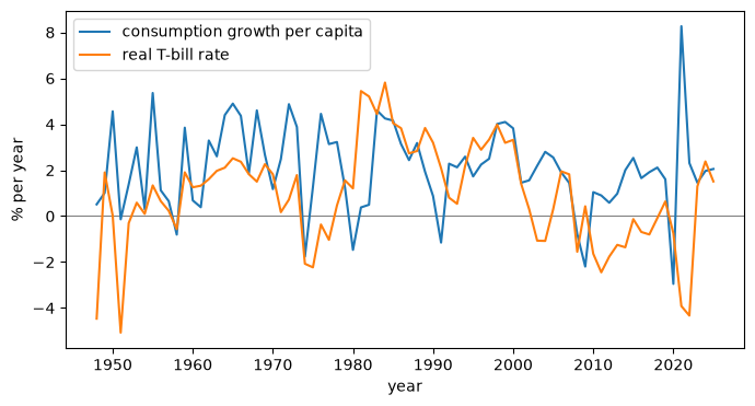
Predict before you plot: if \(\sigma\) were large, how would consumption growth and the real rate move together? Run the next cell and compare.

Code

cons_growth = 100 * np.log(ann.c).diff()
real_rate = ann.i - ann.pi
fig, ax = plt.subplots(figsize=(8, 4))
ax.axhline(0, color="grey", lw=0.8)
ax.plot(cons_growth, label="consumption growth per capita")
ax.plot(real_rate, label="real T-bill rate")
ax.set_xlabel("year"); ax.set_ylabel("% per year"); ax.legend()
plt.show()

Interpret. Find two periods with a negative real rate. What does the Euler equation predict for consumption growth in those years? What actually happened?

🔵 Advanced — Your turn

The self-checks assume the dated snapshot loaded above.

Task 1. Create a DataFrame d from ann with two new columns: gc, consumption growth per capita in % (\(100 \times \Delta \ln c\)), and r, the ex-post real rate in % (T-bill rate i minus inflation pi). Drop rows with missing values.

Code

# YOUR CODE HERE

Code

#@title ✅ Solution (double-click to reveal) { display-mode: "form" }
d = ann.copy()
d["gc"] = 100 * np.log(d.c).diff()
d["r"] = d.i - d.pi
d = d.dropna()

Code

assert len(d) == 78, "Expected 78 complete years (1948–2025). Did you drop missing values?"
assert abs(d.gc.mean() - 2.078) < 0.01, "Mean consumption growth should be about 2.08% — use 100 * np.log(...).diff()."
assert abs(d.r.mean() - 0.941) < 0.01, "Mean real rate should be about 0.94% — subtract inflation from the T-bill rate."
print("✓ Task 1 looks right")

✓ Task 1 looks right

Task 2. Estimate the Euler-equation slope: regress gc on a constant and r with statsmodels OLS. Store the slope in sigma_hat. Is it close to the \(\sigma = 1\) of log utility?

Code

# YOUR CODE HERE

Code

#@title ✅ Solution (double-click to reveal) { display-mode: "form" }
ols = sm.OLS(d.gc, sm.add_constant(d.r)).fit(cov_type="HAC", cov_kwds={"maxlags": 2})
sigma_hat = ols.params["r"]
print(ols.summary().tables[1])

==============================================================================
                 coef    std err          z      P>|z|      [0.025      0.975]
------------------------------------------------------------------------------
const          1.9004      0.242      7.840      0.000       1.425       2.376
r              0.1892      0.123      1.536      0.124      -0.052       0.431
==============================================================================

Code

assert abs(sigma_hat - 0.189) < 0.005, "The slope should be about 0.19 — regress d.gc on sm.add_constant(d.r)."
print(f"✓ Task 2: sigma_hat = {sigma_hat:.2f} — far below 1: intertemporal substitution looks weak (as Hall, 1988, concluded)")

✓ Task 2: sigma_hat = 0.19 — far below 1: intertemporal substitution looks weak (as Hall, 1988, concluded)

Task 3. Is \(r > g\)? Compute share_rg, the percentage of years in which the real rate r exceeds aggregate real GDP growth g.

Code

# YOUR CODE HERE

Code

#@title ✅ Solution (double-click to reveal) { display-mode: "form" }
share_rg = 100 * (d.r > d.g).mean()

Code

assert abs(share_rg - 19.2) < 0.5, "About 19% of years — compare d.r with d.g and take the mean of the boolean."
print(f"✓ Task 3: r > g in {share_rg:.0f}% of years for the SAFE rate. Why might the return on capital differ?")

✓ Task 3: r > g in 19% of years for the SAFE rate. Why might the return on capital differ?

🔴 Frontier — extensions

Instrumental variables. The ex-post real rate is measured with error and timing is blurred by annual averaging. Re-estimate \(\sigma\) using lagged real rates and lagged inflation as instruments (two-stage least squares, e.g. statsmodels.sandbox.regression.gmm.IV2SLS). Does \(\hat\sigma\) change?
Ex-ante real rate. Fetch the University of Michigan inflation expectations series (MICH, monthly, copyrighted, citation required, so fetch it live, don’t redistribute it) and build \(i - \pi^e\).
Which r? Repeat Task 3 with the 10-year Treasury yield (GS10) minus inflation. How does the answer change?

Refresh from source (optional)

The cells above use a dated snapshot so results are reproducible. Call refresh() to fetch today’s data from FRED (no API key needed), then re-run the notebook from the Core section.

Code

def refresh():
    """Fetch the latest FRED data into q, gdp, tb (keyless CSV endpoint)."""
    global q, gdp, tb
    base = "https://fred.stlouisfed.org/graph/fredgraph.csv?id="
    q = pd.read_csv(base + "A794RX0Q048SBEA,PCECTPI", parse_dates=["observation_date"])
    gdp = pd.read_csv(base + "GDPC1", parse_dates=["observation_date"])
    tb = pd.read_csv(base + "TB3MS", parse_dates=["observation_date"])
    print("Fetched up to", q.observation_date.max().date())

Sources and licences

U.S. Bureau of Economic Analysis (A794RX0Q048SBEA, PCECTPI, GDPC1) and Board of Governors of the Federal Reserve System (TB3MS), retrieved from FRED, Federal Reserve Bank of St. Louis, 2026-10-15. Public domain.

Back to the data lab page.