Chapter 3 — The neoclassical growth model: simulate the model

Macroeconomics for Public Policy: A Study Companion to Advanced Macroeconomics. 🟢 see the dynamics · 🔵 comparative statics and “Your turn” tasks · 🔴 solve the model by shooting.

· Study guide

# Setup — numpy, scipy and matplotlib are preinstalled in Colab.
import numpy as np
import matplotlib.pyplot as plt
from scipy import optimize, integrate
np.random.seed(0)
plt.rcParams.update({"figure.figsize": (7, 4.2), "axes.spines.top": False, "axes.spines.right": False})

The model

The next cell is the guide’s canonical model, the same code that draws the guide’s key graphs and checks its exercises. Technology is the chapter’s Cobb–Douglas, \(f(k) = A k^{1-\alpha}\), where \(\alpha\) is the labour share, with no depreciation. The chapter gives no calibration, so the parameters are illustrative.

# Model code — copied verbatim from guides/ch03-the-neoclassical-growth-model/_model.py
"""Canonical model for Chapter 3 — The neoclassical growth model (Ramsey–Cass–Koopmans).

THE single source of the chapter's model equations for this guide: key-graphs.qmd imports it, _verify.py
checks against it, write-notebook copies it verbatim into the model notebook, and _model.js (the OJS
sliders) is checked against it through PARITY_CASES (`uv run m4pp check-parity ch03`).

Notation follows the chapter (book/ch03-the-neoclassical-growth-model/main.md): per-capita capital k,
consumption c, population growth n, rate of time preference rho (> n), elasticity of intertemporal
substitution sigma, NO depreciation (the chapter sets delta = 0, §3.1 "The resource constraint").
Technology is the chapter's Cobb–Douglas, eq. 3.19, Y = A L^alpha K^(1-alpha), where ALPHA IS THE
LABOUR SHARE (eq. 3.21) — so per capita f(k) = A k^(1-alpha).

The chapter gives no calibration: the values below are ILLUSTRATIVE (chosen so rho > n), and every page
that uses them says so.
"""
import numpy as np
from scipy.integrate import solve_ivp

# --- Illustrative parameters (the chapter gives none; rho > n is required, footnote 5) ----------
A = 1.0          # total factor productivity
ALPHA = 2 / 3    # labour share (eq. 3.21); the capital share is 1 - ALPHA
RHO = 0.04       # rate of time preference
N = 0.01         # population growth
SIGMA = 1.0      # elasticity of intertemporal substitution (eq. 3.13); 1 = log utility


def f(k, A=A, alpha=ALPHA):
    """Output per capita, f(k) = A k^(1-alpha)."""
    return A * np.power(k, 1 - alpha)


def f_prime(k, A=A, alpha=ALPHA):
    """Marginal product of capital, f'(k) = (1-alpha) A k^(-alpha)."""
    return (1 - alpha) * A * np.power(k, -alpha)


def f_second(k, A=A, alpha=ALPHA):
    """f''(k) = -alpha (1-alpha) A k^(-alpha-1) < 0 (diminishing returns)."""
    return -alpha * (1 - alpha) * A * np.power(k, -alpha - 1)


def k_star(rho=RHO, A=A, alpha=ALPHA):
    """Steady-state capital from the modified golden rule f'(k*) = rho (eq. 3.17)."""
    return ((1 - alpha) * A / rho) ** (1 / alpha)


def k_golden(n=N, A=A, alpha=ALPHA):
    """Golden-rule capital from f'(k_G) = n (eq. 3.18): maximises steady-state consumption."""
    return ((1 - alpha) * A / n) ** (1 / alpha)


def c_kdot0(k, n=N, A=A, alpha=ALPHA):
    """The kdot = 0 locus, c = f(k) - n k (eq. 3.16): hump-shaped, peaking at k_G."""
    return f(k, A, alpha) - n * k


def c_star(rho=RHO, n=N, A=A, alpha=ALPHA):
    """Steady-state consumption: the kdot = 0 locus evaluated at k* (eqs. 3.16–3.17)."""
    return c_kdot0(k_star(rho, A, alpha), n, A, alpha)


def euler_growth(k, rho=RHO, sigma=SIGMA, A=A, alpha=ALPHA):
    """Consumption growth from the Euler equation, cdot/c = sigma [f'(k) - rho] (eq. 3.15)."""
    return sigma * (f_prime(k, A, alpha) - rho)


def eigenvalues(rho=RHO, n=N, sigma=SIGMA, A=A, alpha=ALPHA):
    """Eigenvalues (stable, unstable) of the linearised system, Omega in eq. 3.33.

    Omega = [[rho - n, -1], [sigma c* f''(k*), 0]];  det = sigma c* f''(k*) < 0 ⇒ opposite signs.
    """
    ks, cs = k_star(rho, A, alpha), c_star(rho, n, A, alpha)
    tr, det = rho - n, sigma * cs * f_second(ks, A, alpha)
    disc = np.sqrt(tr ** 2 - 4 * det)
    return (tr - disc) / 2, (tr + disc) / 2


def eig_stable(rho=RHO, n=N, sigma=SIGMA, A=A, alpha=ALPHA):
    """The negative (stable) eigenvalue: the speed at which the economy converges along the saddle path."""
    return eigenvalues(rho, n, sigma, A, alpha)[0]


def saddle_slope(rho=RHO, n=N, sigma=SIGMA, A=A, alpha=ALPHA):
    """Slope dc/dk of the saddle path at the steady state (linear approximation): rho - n - lambda_s > 0."""
    return rho - n - eig_stable(rho, n, sigma, A, alpha)


def dynamics(t, y, rho=RHO, n=N, sigma=SIGMA, A=A, alpha=ALPHA):
    """The system eqs. 3.5 and 3.15: kdot = f(k) - n k - c,  cdot = sigma c [f'(k) - rho]."""
    k, c = y
    return [f(k, A, alpha) - n * k - c, sigma * c * (f_prime(k, A, alpha) - rho)]


def saddle_path(k_min, k_max, rho=RHO, n=N, sigma=SIGMA, A=A, alpha=ALPHA, eps=1e-4):
    """Global saddle path c(k) on [k_min, k_max], traced by integrating the system BACKWARD in time
    from points just off the steady state along the stable eigenvector (backward, the stable arm
    becomes the attracting one). Returns (k, c) sorted by k."""
    ks, cs = k_star(rho, A, alpha), c_star(rho, n, A, alpha)
    slope = saddle_slope(rho, n, sigma, A, alpha)
    pieces = []
    for direction in (-1, 1):
        k0, c0 = ks + direction * eps * ks, cs + direction * eps * ks * slope
        stop = (lambda t, y: y[0] - k_min) if direction < 0 else (lambda t, y: y[0] - k_max)
        stop.terminal = True
        sol = solve_ivp(lambda t, y: [-v for v in dynamics(t, y, rho, n, sigma, A, alpha)],
                        (0, 2000), [k0, c0], events=stop, max_step=1.0, rtol=1e-9, atol=1e-11)
        pieces.append(sol.y)
    k = np.concatenate([pieces[0][0][::-1], [ks], pieces[1][0]])
    c = np.concatenate([pieces[0][1][::-1], [cs], pieces[1][1]])
    keep = (k > 0) & (c > 0)
    order = np.argsort(k[keep])
    return k[keep][order], c[keep][order]


def transition(k0, T=200, rho=RHO, n=N, sigma=SIGMA, A=A, alpha=ALPHA, num=401):
    """Optimal paths (t, k_t, c_t) from k0: consumption jumps onto the saddle path, then both move
    together to the steady state (policy function c(k) from the saddle path)."""
    ks = k_star(rho, A, alpha)
    kp, cp = saddle_path(min(k0, ks) * 0.5, max(k0, ks) * 1.5, rho, n, sigma, A, alpha)
    policy = lambda k: np.interp(k, kp, cp)
    sol = solve_ivp(lambda t, y: [f(y[0], A, alpha) - n * y[0] - policy(y[0])], (0, T), [k0],
                    t_eval=np.linspace(0, T, num), rtol=1e-9, atol=1e-11)
    k = sol.y[0]
    return sol.t, k, policy(k)

🟢 Core — see the dynamics

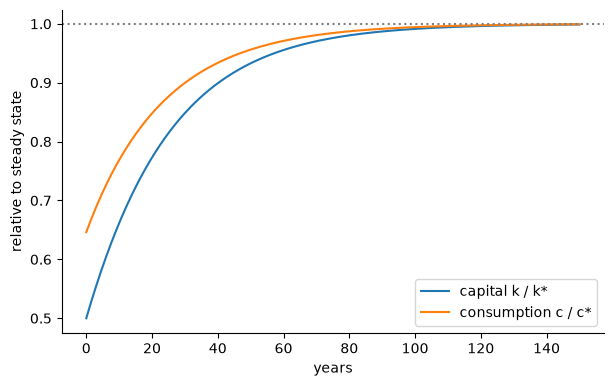
An economy starts with half the steady-state capital stock. Consumption jumps onto the saddle path; then capital and consumption rise together towards the steady state \((k^*, c^*)\).

ks, cs = k_star(), c_star()
t, kt, ct = transition(0.5 * ks, T=150)
fig, ax = plt.subplots()
ax.plot(t, kt / ks, label="capital k / k*")
ax.plot(t, ct / cs, label="consumption c / c*")
ax.axhline(1, color="grey", ls=":")
ax.set_xlabel("years"); ax.set_ylabel("relative to steady state"); ax.legend()
plt.show()
print(f"k* = {ks:.2f}, c* = {cs:.3f}; consumption starts at {ct[0] / cs:.0%} of c*")

k* = 24.06, c* = 2.646; consumption starts at 65% of c*

What you see. Capital is below its steady state, so its marginal product exceeds \(\rho\): the Euler equation says consumption must grow, and it does, together with capital. Consumption starts below \(c^*\) because it jumped onto the saddle path, which lies below the \(\dot k = 0\) locus to the left of \(k^*\).

Questions. 1. Why can’t capital jump to \(k^*\) immediately? 2. Why doesn’t consumption start at \(c^*\)?

🔵 Advanced — comparative statics

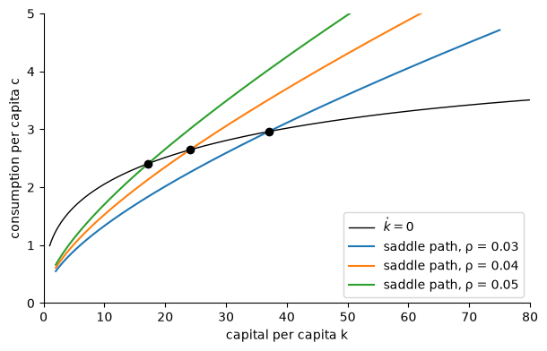
Three economies differ only in patience \(\rho\). More patient economies (lower \(\rho\)) accumulate more capital: the \(\dot c = 0\) line, and with it the saddle path, moves right.

fig, ax = plt.subplots()
k = np.linspace(1, 80, 300)
ax.plot(k, c_kdot0(k), color="black", lw=1, label=r"$\dot k = 0$")
for rho in (0.03, 0.04, 0.05):
    kp, cp = saddle_path(2, 75, rho=rho)
    ax.plot(kp, cp, label=f"saddle path, ρ = {rho}")
    ax.plot([k_star(rho)], [c_star(rho)], "o", color="black")
ax.set_xlim(0, 80); ax.set_ylim(0, 5)
ax.set_xlabel("capital per capita k"); ax.set_ylabel("consumption per capita c"); ax.legend()
plt.show()

Your turn 1

Compute the steady-state capital stock when \(\rho = 0.05\) (other parameters unchanged) and store it in k_ss_high_rho. Is it higher or lower than the baseline \(k^*\) (with \(\rho = 0.04\))?

# YOUR CODE HERE

#@title ✅ Solution (double-click to reveal) { display-mode: "form" }
k_ss_high_rho = k_star(rho=0.05)
print(f"k* with rho = 0.05: {k_ss_high_rho:.2f} (baseline {k_star():.2f})")

k* with rho = 0.05: 17.21 (baseline 24.06)

assert abs(k_ss_high_rho - ((1 / 3) / 0.05) ** 1.5) < 1e-9, "Use k_star(rho=0.05): the modified golden rule f'(k*) = rho."
print("✓ Your turn 1 looks right — more impatience, less capital")

✓ Your turn 1 looks right — more impatience, less capital

Your turn 2

The speed of convergence is \(|\lambda_s|\), so the half-life of a gap is \(\ln 2 / |\lambda_s|\). Compute the half-life for \(\sigma = 0.5\) and for \(\sigma = 2\); store them in half_life_low and half_life_high. Which economy converges faster, and why?

# YOUR CODE HERE

#@title ✅ Solution (double-click to reveal) { display-mode: "form" }
half_life_low = np.log(2) / abs(eig_stable(sigma=0.5))
half_life_high = np.log(2) / abs(eig_stable(sigma=2.0))
print(f"half-life: sigma = 0.5 → {half_life_low:.1f} years; sigma = 2 → {half_life_high:.1f} years")

half-life: sigma = 0.5 → 26.5 years; sigma = 2 → 11.0 years

assert half_life_high < half_life_low, "A higher sigma should mean FASTER convergence (shorter half-life)."
assert abs(half_life_low - np.log(2) / abs(eigenvalues(sigma=0.5)[0])) < 1e-9, "Use eig_stable(sigma=...)."
print("✓ Your turn 2 looks right — households willing to shift consumption over time adjust faster")

✓ Your turn 2 looks right — households willing to shift consumption over time adjust faster

🔴 Frontier — solve the model by shooting

saddle_path traces the saddle path by integrating backward from the steady state. Here we solve it the other way: forward shooting. Fix \(k_0\) and bisect on \(c_0\). If \(c_0\) is too high, capital runs out; if it is too low, capital over-accumulates. The bracket closes on the saddle path.

def fate(c0, k0, T=600):
    """+1 if capital runs out (c0 too high), -1 otherwise (c0 too low or on the path)."""
    zero = lambda t, y: y[0] - 0.5 * k0; zero.terminal = True
    over = lambda t, y: y[0] - 3 * k_star(); over.terminal = True
    sol = integrate.solve_ivp(dynamics, (0, T), [k0, c0], events=[zero, over], rtol=1e-10)
    return 1 if sol.t_events[0].size else -1

k0 = 0.5 * k_star()
lo, hi = 0.1, c_kdot0(k0)
for _ in range(60):
    mid = (lo + hi) / 2
    lo, hi = (lo, mid) if fate(mid, k0) > 0 else (mid, hi)
c0_shoot = (lo + hi) / 2
kp, cp = saddle_path(2, 75)
print(f"shooting: c0 = {c0_shoot:.5f}   backward saddle path: c0 = {np.interp(k0, kp, cp):.5f}")

shooting: c0 = 1.70998   backward saddle path: c0 = 1.70993

Two independent methods agree on the saddle path, which is how the guide’s verification script checks its own numbers.

Extensions. 1. Add depreciation \(\delta\): change the resource constraint to \(\dot k = f(k) - (n+\delta)k - c\). How do \(k^*\) and the golden rule change? 2. Simulate an anticipated permanent fall in \(\rho\) announced at \(t = 0\) but effective at \(t = 10\). Consumption should jump only at \(t = 0\).

---

Keep going: Key graphs · Exercises · Derivations · Data lab