Regional growth, convergence, and spatial spillovers in India: A reproducible view from outer space

1 Introduction

Regional growth and convergence matter most in federal states such as India. In such settings, spatial inequalities can threaten social cohesion and political stability. Consistent economic data, however, are rarely available below the state level. Satellite nighttime lights have relaxed that constraint by serving as a proxy for economic activity. Using those data, Chanda and Kabiraj (2020) document convergence across 520 Indian districts between 1996 and 2010. However, their analysis does not account for spatial spillovers. Such spillovers can arise from the diffusion of technology and from the movement of resources across neighboring districts.

This article extends that analysis along three dimensions. The first is replication: we adopt the data, the sample, and the conditioning variables of Chanda and Kabiraj (2020) without modification, so that any difference in the estimates reflects the spatial modeling alone. The second is substantive: we build an interactive visualization of regional convergence, test formally for spatial dependence, and estimate a spatial Durbin model. The model shows that catch-up across Indian districts has a significant neighborhood dimension. The spatial spillover effect of initial luminosity is negative and statistically significant. Districts whose neighbors started from a lower base therefore grew faster than their own initial conditions alone would predict.

The third contribution is methodological, and it is the primary one. This article shows that a comprehensive spatial econometric study can be implemented using only open-source software and cloud computing. Our workflow covers every step, from visualizing the satellite imagery and constructing the neighborhood structure to testing for spatial dependence, modeling the spillovers, and running the robustness checks.

That workflow delivers the main empirical result of the article. Accounting for spatial spillovers raises the estimated speed of regional convergence from about 3.0% to about 5.2% per year. The implied half-life of regional disparities therefore falls from roughly 23 years to 13. The same workflow extends beyond economic output, and we illustrate that reach with an exploratory analysis of luminosity and cultural participation across Indian states. Our results suggest that luminosity is positively associated with media-based cultural consumption and negatively associated with community-based participation. This pattern is consistent with luminosity tracking electrification and urbanization rather than economic output alone.

Every figure and table in this article is produced by one of the six cloud-based computational scripts and notebooks listed in Table 1. The five analytical notebooks are written in Python and run in Google Colaboratory, so a reader needs no local installation and no licensed software: clicking Run all downloads the data and re-executes the analysis. The remaining notebook, N1, hosts the interactive visualization and its Google Earth Engine source code. The notebooks, the data, and the manuscript source are in the project repository at https://github.com/quarcs-lab/project2025s-py, and their rendered versions are embedded in the online edition at https://quarcs-lab.github.io/project2025s-py/.

Table 1: Computational notebooks and scripts underlying this article

Notebook	Content
N1. View from outer space	Interactive luminosity map with Earth Engine script
N2. Regional convergence	Luminosity growth on initial luminosity, with speed and half-life
N3. Spatial dependence	Weight matrices, Global Moran’s I, and LISA cluster maps
N4. Spillover modeling	OLS and spatial Durbin estimates, impacts, and convergence speeds
N5. Robustness	Model 4 under six alternative weight matrices
N6. Spatial culture	Luminosity and cultural participation across Indian states

The rest of this article is organized as follows. Section 2 describes the data and the methods, and Section 3 presents the empirical results. Section 4 discusses the policy implications, the extension to multiple periods, the analysis of cultural participation, and new directions for research. Section 5 offers concluding remarks.

2 Data and methods

2.1 Data: Nighttime lights as a proxy for economic activity

Satellite images of nighttime light provide a proxy for economic activity below the national level. Henderson, Storeygard, and Weil (2012) pioneered this approach in economics. Their work exploits the empirical correlation between the intensity of artificial light observed from space and economic output on the ground. X. Chen and Nordhaus (2011) show that the proxy is most informative where official statistics are of low quality. Nighttime light (hereafter NTL) data have therefore become a standard tool for the study of growth and convergence across national and subnational regions.

NTL data have been applied to a wide range of questions in development economics. One line of work studies the effect of decentralization on regional convergence (Adhikari and Dhital 2021). A second line adjudicates between national accounts and household surveys, and it finds that national accounts track the light data more closely (Pinkovskiy and Sala-i-Martin 2016). A third line estimates GDP per capita and spatial inequality at the global scale (Lessmann and Seidel 2017). The Indian literature is equally varied, and it covers welfare programs, colonial institutions, demonetization, and the pandemic.¹ Chakravarty and Dehejia (2017) document large regional disparities in India and caution that the goods and services tax may widen them further. Taken together, these studies show that NTL data are well suited to the analysis of subnational disparities.

Our empirical design follows Chanda and Kabiraj (2020). The dependent variable is the growth rate of nighttime lights per capita. The primary explanatory variable is the initial level of nighttime lights per capita. We construct both variables for 520 districts in India from data released by the National Geophysical Data Center (NGDC). These data record observations from the DMSP-OLS satellites over the period from 1996 to 2010. To mitigate top-coding in brightly lit areas, the NGDC also released a radiance-calibrated series for eight specific years, which combines high magnification settings for low-light regions with low magnification settings for bright ones. Six of those eight years fall inside our 1996–2010 sample window, and they are the dates our dataset holds. In this article, we use the radiance-calibrated series throughout.²

2.2 A reproducible workflow and interactive visualization

We implement the entire study in a reproducible workflow. Jupyter notebooks combine executable code, explanatory narrative, and computational output in a single document (Kluyver et al. 2016), which is the practical expression of literate programming (Knuth 1984). We document the data processing, the estimation, and the visualization in notebooks that run on a single Python kernel. Each result can therefore be traced to the code that produced it. Quarto then extends those notebooks into a manuscript framework (Allaire et al. 2024). Every figure and table is embedded from an identified notebook cell, and one source file generates the HTML, PDF, Word, and JATS XML versions without discrepancies between them. The toolchain is open source, and the data and code are public (Peng 2011). Each notebook also runs in the cloud on Google Colaboratory, which requires no local installation. Readers can therefore re-execute the whole pipeline in a browser and without proprietary software.

Satellite data have opened new dimensions of economic measurement (Donaldson and Storeygard 2016). Interactive visualization complements that measurement, because it reveals spatial and temporal heterogeneity that static maps obscure. Google Earth Engine lowers the computational barriers to such visualization (Gorelick et al. 2017). Its browser-based environment requires no local software, and its catalog already holds the DMSP-OLS and VIIRS nighttime lights collections (Tamiminia et al. 2020). Readers can therefore track light intensity across regions over time, and they can see where initially dim regions brightened fastest. That pattern is the visual counterpart of the convergence relationship estimated in Section 3.

2.3 Regional convergence modeling

Neoclassical growth theory predicts that poor regions grow faster than rich ones. Diminishing returns to capital accumulation make the per capita growth rate of a region negatively correlated with its initial endowment (Solow 1956). Regions that share technology and preferences should therefore converge to a common steady state in the long run. We test that prediction within the growth regression framework of Barro and Sala-i-Martin (1992). Equation 1 states the convergence process in its simplest unconditional form.

\[ \boldsymbol{g_t} = \beta_1 \boldsymbol{x_{t-1}} + \boldsymbol{\varepsilon_t} \tag{1}\]

where \(\boldsymbol{g_t}\) is an \(N\text{-by-}1\) vector of per-capita NTL growth for the \(N\) regions over the period \(t\). The vector \(\boldsymbol{x_{t-1}}\) collects the initial (log) per-capita NTL of the same regions, and \(\boldsymbol{\varepsilon_t}\) collects idiosyncratic error terms. The parameter \(\beta_1\) measures the direction and the strength of regional convergence. A negative value implies that regions with lower initial NTL levels grow faster, which is the convergence hypothesis.

The estimated convergence coefficient translates into two quantities that are easier to interpret (Barro and Sala-i-Martin 1992). The first is the annual speed of convergence, and the second is the half-life. Because the dependent variable is average annual growth over \(T\) years, the implied convergence speed is \(\lambda = -\ln(1 + \beta_1 T)/T\). The half-life is \(\ln(2)/\lambda\), which is the time required to close half of the initial gap to the steady state. In our application \(T = 14\) years. We apply the same transformation to the total effect of initial luminosity in the spatial models.

The unconditional framework contains no control variables, so it imposes a common steady state on every region. That assumption is restrictive, because regions differ in geography, in socioeconomic conditions, and in policy implementation. We therefore add state fixed effects, which absorb state-specific institutions and policies. We also add geo-climatic controls and district-specific conditions related to demographics, human capital, and infrastructure. Equation 2 summarizes the resulting conditional convergence framework.

\[ \boldsymbol{g_t} = \beta_1 \boldsymbol{x_{t-1}} + \boldsymbol{X_t} \boldsymbol{\alpha} + \boldsymbol{\varepsilon_t} \tag{2}\]

Here, the matrix \(\boldsymbol{X_t}\) is an \(N\text{-by-}k\) collection of observations on control variables for each district in our sample, and it includes the state fixed effects. The vector \(\boldsymbol{\alpha}\), with dimensions \(k\text{-by-}1\), collects the associated regression coefficients. The conditioning set is adopted unchanged from Chanda and Kabiraj (2020). That choice is deliberate, because the present analysis extends that study rather than replacing it. Holding the controls fixed ensures that any difference between our estimates and their estimates comes from the spatial specification and not from a different choice of covariates.

The 16 district-level controls fall into three groups.³ Geography and agro-climate capture slow-moving determinants of the steady state that do not vary over the sample period. Demographics and human capital capture the factor endowments through which districts accumulate. Infrastructure captures access to the electricity grid and to markets. This last group matters here, because luminosity is itself partly a measure of electrification. The conditional models therefore compare districts that began the period with similar levels of grid access.

The demographic, human-capital, and electrification controls are measured in 1996, at the start of the growth period. They are therefore predetermined with respect to subsequent growth. The paved-roads variable is measured in 2000. The full list of control variables, with their measurement years and summary statistics, is given in Table A.1 of Chanda and Kabiraj (2020).

We estimate both specifications on a single long difference. The dependent variable is average annual growth between 1996 and 2010, and the regressors are measured at the start of that period. This is the design of Chanda and Kabiraj (2020), and we retain it. The design identifies the average rate at which districts converged over fourteen years. It is silent, however, on how that rate evolved within the period. We return to this limitation, and to what a panel design would require, in the discussion.

2.4 Spatial dependence testing

Spatial dependence is the tendency for observations at nearby locations to be more similar than observations at distant locations. It can arise from spatial spillovers, from shared geographic conditions, or from inter-regional economic linkages (Anselin 1988). When it is present and left unmodeled, standard regressions yield biased parameter estimates and invalid inference. We therefore test for spatial dependence with the Global Moran’s I statistic and with Local Indicators of Spatial Association (LISA). We apply both tests to the main variables of Equation 2.

The Global Moran’s I statistic quantifies the overall degree of spatial clustering among geographic units (Moran 1950). It compares the deviation of each observation from the mean with the deviations of its neighbors. Equation 3 gives the formula.

\[ I=\frac{n}{\sum_i \sum_j w_{ij}} \cdot \frac{\sum_i \sum_j w_{ij} \, z_i \, z_j}{\sum_i z_i^2} \tag{3}\]

where \(z_i\) is the deviation of observation \(i\) from the mean, and \(w_{ij}\) is the spatial weight that connects units \(i\) and \(j\). The term \(n\) denotes the total number of observations. The statistic typically ranges from \(-1\) to \(+1\). Positive values indicate that similar values tend to be located near each other.⁴ We assess significance with a permutation-based inference approach.⁵

The global statistic does not reveal where the clusters and outliers are located. Anselin (1995) therefore proposed Local Indicators of Spatial Association, which decompose the global statistic into a contribution from each observation. Equation 4 defines the local statistic for observation \(i\).

\[ I_i = z_i \sum_j w_{ij} \, z_j \tag{4}\]

where the summation is over the neighbors of \(i\), as defined by the spatial weight matrix. Each observation is then classified into one of four categories, according to how its value relates to the values of its neighbors. The High-High and Low-Low categories identify spatial clusters, and the High-Low and Low-High categories identify spatial outliers.⁶ We assess significance with conditional permutation tests. The LISA cluster maps report only the significant locations, typically at \(p < 0.05\).

The spatial weight matrix \(\mathbf{W}\) determines which districts are treated as neighbors, so its specification is central to the analysis. We employ a six-nearest-neighbor (6NN) matrix. It sets \(w_{ij} = 1\) if district \(j\) is among the six nearest districts to \(i\) by centroid distance, and \(w_{ij} = 0\) otherwise.⁷ Each district therefore has the same number of neighbors, even though district sizes vary widely across the country. We then row-normalize the matrix, as is standard practice, so that each row sums to one. The spatial lag \(\mathbf{W} \mathbf{x}\) is then the average value among the neighbors of a district.

The choice of \(k = 6\) balances two concerns. It is large enough to capture local spatial interactions, and it is small enough to exclude distant districts that are unlikely to exert economic influence. The data also support this choice. Among the seven weight matrices considered in Table 4, the 6NN specification attains the lowest AIC, which indicates the best fit to the spatial structure of the data. We nevertheless treat the definition of the neighborhood as an open question. In Section 3 we re-estimate the preferred model under six alternative weight matrices, which range from contiguity-based schemes to inverse-distance schemes. Those results, reported in Figure 8 and Table 4, show that the direct and total convergence effects do not depend on this choice.

Evidence of significant spatial dependence would justify the use of spatial econometric methods. Ertur and Koch (2007) argue that the spatial Durbin model (SDM) accounts for such dependence in the convergence process. Fischer (2011) derives the same specification as the reduced form of a spatially interdependent growth model. The SDM also separates the direct effects of district characteristics from the indirect effects that operate through spatial channels (LeSage and Pace 2009).

2.5 Spatial spillover modeling

Our spatial spillover modeling builds on the spatially augmented Solow model of Ertur and Koch (2007), which was developed for countries. It also builds on the regional Mankiw-Romer-Weil extension of that model by Fischer (2011). Both models account for technological interdependence across economies. We apply this framework to an economy of \(N\) subnational regions. Each region is characterized by the Cobb-Douglas production function with constant returns to scale in Equation 5.

\[ Y_{i t}=A_{i t} K_{i t}^{\alpha_{K}} H_{i t}^{\alpha_{H}} L_{i t}^{1-\alpha_{K} -\alpha_{H}} \tag{5}\]

where \(Y_{it}\) is output, \(K_{it}\) is physical capital, \(H_{it}\) is human capital, \(L_{it}\) is the labor force, and \(A_{it}\) is the level of technological knowledge for region \(i\) at time \(t\). The parameters \(\alpha_K\) and \(\alpha_H\) are the output elasticities with respect to physical and human capital. Technological knowledge is not exogenous in this framework, because it depends on internal and on external factors. Equation 6 states that relation.

\[ A_{i t}=\Omega_{t} k_{i t}^{\theta} h_{i t}^{\phi} \prod_{j \neq i}^{N} A_{j t}^{\rho W_{i j}} \tag{6}\]

The specification captures three components of technological progress:

• An exogenous component (\(\Omega_t\)) that represents the common stock of knowledge across regions.
• An embodied component (\(k_{i t}^{\theta} h_{i t}^{\phi}\)) that reflects technology embedded in physical and human capital per worker.
• A spatial component (\(\prod_{j \neq i}^{N} A_{j t}^{\rho W_{i j}}\)) that captures technological interdependence between regions.

The third component is absent from the standard Solow model, and it is the source of the spatial spillovers in growth.

From this framework Ertur and Koch (2007) derived a spatial Durbin model that accounts for spillovers in the convergence process, with the human-capital terms following Fischer (2011). The model augments the conditional specification of Equation 2 with spatial lags of the dependent variable, of initial luminosity, and of the control variables, and can be written compactly as Equation 7:

\[ \boldsymbol{g_t} = \beta_1 \boldsymbol{x_{t-1}} + \boldsymbol{X_t} \boldsymbol{\alpha} + \beta_2 \boldsymbol{W} \boldsymbol{x_{t-1}} + \boldsymbol{W} \boldsymbol{X_t} \boldsymbol{\gamma} + \rho \boldsymbol{W} \boldsymbol{g_t} + \boldsymbol{\varepsilon_t} \tag{7}\]

The vectors \(\boldsymbol{g_t}\), \(\boldsymbol{x_{t-1}}\) and \(\boldsymbol{\varepsilon_t}\), the matrix \(\boldsymbol{X_t}\), and the parameters \(\beta_1\) and \(\boldsymbol{\alpha}\) are defined as in Equation 2 above. The new terms are the spatial lags: \(\boldsymbol{W} \boldsymbol{x_{t-1}}\) and \(\boldsymbol{W} \boldsymbol{g_t}\) are \(N\text{-by-}1\) vectors of neighborhood averages of initial luminosity and of growth, while \(\boldsymbol{W} \boldsymbol{X_t}\) is the corresponding \(N\text{-by-}k\) matrix for the control variables. The coefficients \(\beta_2\), \(\boldsymbol{\gamma}\) and \(\rho\) measure how strongly each of these neighborhood averages enters the growth of a district.⁸

3 Results

3.1 Regional convergence: An interactive exploration from outer space

Before presenting the regression results, we illustrate growth and convergence in nighttime lights visually, through an interactive map of India, a convergence scatterplot, and case studies of some of the poorest regions of the country.⁹

Figure 1: Regional luminosity in India: 1996 vs 2010
Notes: Luminosity is measured in radiance-calibrated digital number (DN) values from DMSP-OLS satellites. Interactive web application available at https://bit.ly/india-rc-ntl.
Source: Authors’ visualization using pre-processed luminosity images from the Earth Observation Group (NOAA/NCEI). See View from outer space notebook for source code.

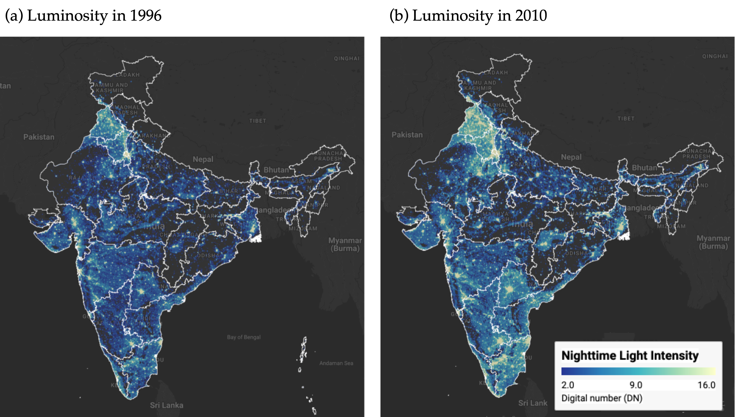
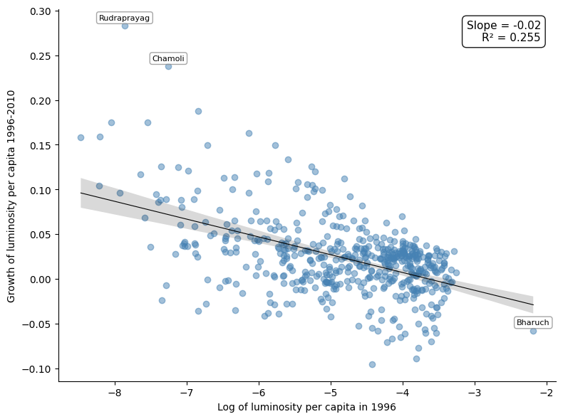
Figure 1 presents static maps of luminosity in the initial and final years, 1996 and 2010, captured from our interactive application. The maps show a noticeable increase in brightness across most of India by 2010, which, since nighttime lights proxy for economic activity, reflects economic growth over the period. Figure 2 then relates per-capita growth in nighttime lights to initial per-capita luminosity, and the relationship is inverse: the estimated \(\beta\)-convergence coefficient of about \(-0.02\) implies an annual speed of convergence of roughly 2.3% and a half-life of about 30 years, consistent with the seminal finding of Barro and Sala-i-Martin (1992). Because \(\beta\)-convergence need not imply a narrowing of the distribution, we also check \(\sigma\)-convergence: the cross-district standard deviation of log per-capita luminosity falls from 1.09 in 1996 to 0.95 in 2010, a reduction of 13.5%, so spatial disparities did narrow over the period.

In [1]:

# Identify outlier districts for labeling
mask = (
    ((data["log_light96_rcr_cap"] > -3) & (data["light_growth96_10rcr_cap"] < 0))
    | ((data["log_light96_rcr_cap"] < -7) & (data["light_growth96_10rcr_cap"] > 0.2))
)
outliers = data[mask]

# Annotated scatterplot
fig, ax = plt.subplots(figsize=(8, 6))
sns.regplot(
    data=data,
    x="log_light96_rcr_cap",
    y="light_growth96_10rcr_cap",
    ci=95,
    scatter_kws={"alpha": 0.5, "color": "steelblue"},
    line_kws={"color": "black", "linewidth": 0.8},
    ax=ax,
)

# Label outlier districts
for _, r in outliers.iterrows():
    ax.annotate(
        r["district"],
        xy=(r["log_light96_rcr_cap"], r["light_growth96_10rcr_cap"]),
        xytext=(0, 6),
        textcoords="offset points",
        ha="center",
        fontsize=8,
        bbox=dict(boxstyle="round,pad=0.3", fc="white", ec="gray", alpha=0.7),
    )

# Slope / R-squared / speed / half-life annotation box (top-right corner)
annotation = "Slope = {}\nR² = {}\nSpeed = {:.1%} per year\nHalf-life = {:.1f} years".format(
    slope, rsq, speed, half_life
)
ax.annotate(
    annotation,
    xy=(0.97, 0.97),
    xycoords="axes fraction",
    ha="right",
    va="top",
    fontsize=11,
    bbox=dict(boxstyle="round,pad=0.4", fc="white", ec="black", alpha=0.9),
)

ax.set_xlabel("Log of luminosity per capita in 1996")
ax.set_ylabel("Growth of luminosity per capita 1996-2010")
sns.despine(ax=ax)
plt.tight_layout()
plt.show()

Figure 2: Regional luminosity convergence across districts in India
Notes: Each point represents one of the 520 districts. The regression line shows the estimated beta-convergence relationship, and the annotation reports its slope, the R-squared, the implied annual speed of convergence, and the half-life. Outlier districts are labeled.
Source: Data from Chanda and Kabiraj (2020). See Regional convergence notebook for source code.

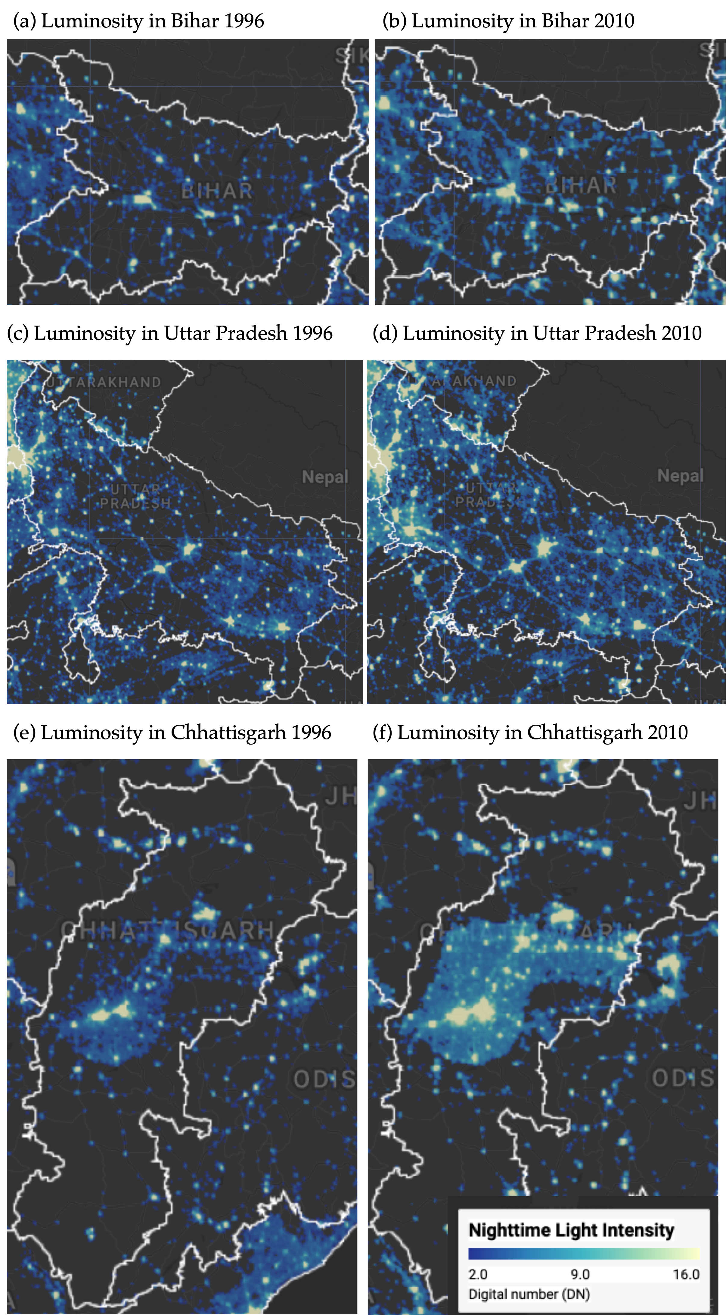
Figure 3 displays the change in luminosity over the study period in three economically disadvantaged states. Bihar is the poorest of them, with a per-capita income at 31.2% of the national average, while Uttar Pradesh and Chhattisgarh stand at 55.3% and 59.9% respectively.¹⁰ All three remain among the poorest states, but all three brightened noticeably over the period.

Figure 3: Some illustrative examples of regional convergence
Notes: Luminosity is measured in radiance-calibrated digital number (DN) values from DMSP-OLS satellites. Interactive web application available at https://bit.ly/india-rc-ntl.
Source: Authors’ visualization using pre-processed luminosity images from the Earth Observation Group (NOAA/NCEI). See View from outer space notebook for source code.

3.2 Spatial dependence is a feature of the convergence process

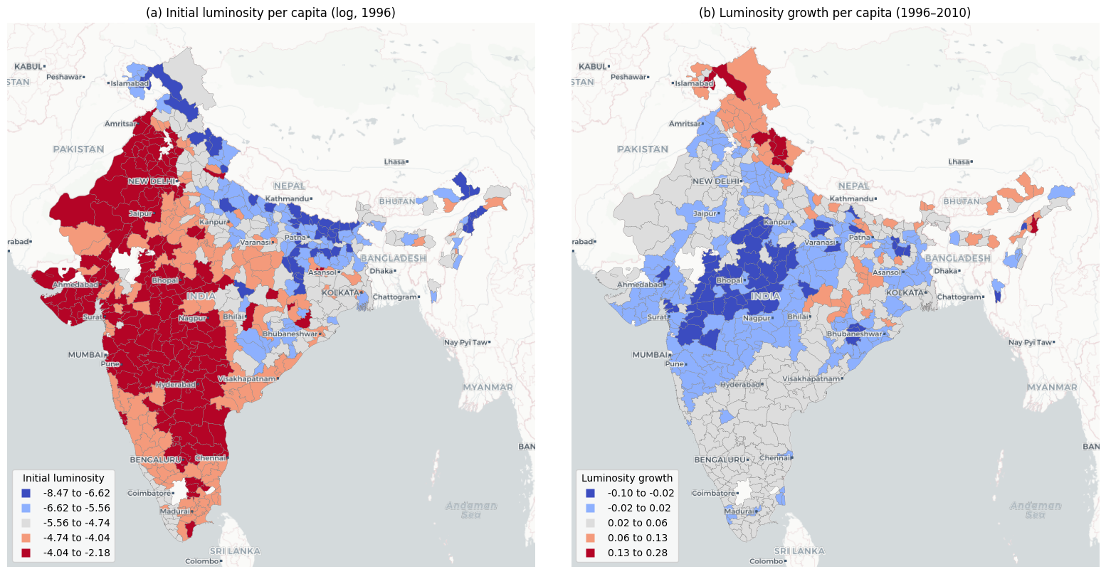
Before the formal econometric analysis, we examine the spatial distribution of the variables under study. Figure 4 maps initial luminosity in 1996 and the subsequent growth rate of luminosity over the 1996–2010 period across the 520 districts in our sample.

In [2]:

# Reproject once to Web Mercator for basemap overlay
_gdf = gdf.to_crs(epsg=3857).copy()

# Classify both variables (Fisher-Jenks, k=5)
clf_init = mc.FisherJenks(_gdf["log_initial"], k=5)
clf_growth = mc.FisherJenks(_gdf["growth"], k=5)

_gdf["init_class"] = clf_init.yb
_gdf["growth_class"] = clf_growth.yb

# Discrete colormap with 5 bins (close to the interactive map style)
cmap = plt.get_cmap("coolwarm", 5)
bounds = np.arange(-0.5, 5.5, 1)
norm = mcolors.BoundaryNorm(bounds, cmap.N)

# Plot: two panels
fig, ax = plt.subplots(1, 2, figsize=(16, 8))

# Left: initial luminosity (log)
_gdf.plot(
    column="init_class",
    cmap=cmap,
    norm=norm,
    linewidth=0.25,
    edgecolor="gray",
    ax=ax[0],
)
cx.add_basemap(ax[0], source=cx.providers.CartoDB.Positron, attribution=False)
cx.add_basemap(ax[0], source=cx.providers.CartoDB.PositronOnlyLabels, attribution=False)
ax[0].set_axis_off()
ax[0].set_title("(a) Initial luminosity per capita (log, 1996)")

# Right: growth
_gdf.plot(
    column="growth_class",
    cmap=cmap,
    norm=norm,
    linewidth=0.25,
    edgecolor="gray",
    ax=ax[1],
)
cx.add_basemap(ax[1], source=cx.providers.CartoDB.Positron, attribution=False)
cx.add_basemap(ax[1], source=cx.providers.CartoDB.PositronOnlyLabels, attribution=False)
ax[1].set_axis_off()
ax[1].set_title("(b) Luminosity growth per capita (1996–2010)")

# Legends (one per panel, with variable-specific breaks)
handles = [
    plt.Line2D([0], [0], marker='s', linestyle='', markersize=9,
               markerfacecolor=cmap(i), markeredgecolor='none')
    for i in range(5)
]

# Left legend labels
init_min = float(_gdf["log_initial"].min())
init_labels = [
    f"{(clf_init.bins[i-1] if i>0 else init_min):.2f} to {clf_init.bins[i]:.2f}"
    for i in range(5)
]
ax[0].legend(handles, init_labels, title="Initial luminosity", loc="lower left", frameon=True)

# Right legend labels
growth_min = float(_gdf["growth"].min())
growth_labels = [
    f"{(clf_growth.bins[i-1] if i>0 else growth_min):.2f} to {clf_growth.bins[i]:.2f}"
    for i in range(5)
]
ax[1].legend(handles, growth_labels, title="Luminosity growth", loc="lower left", frameon=True)

plt.tight_layout()
plt.show()

Figure 4: Spatial distribution of initial luminosity and luminosity growth
Notes: Districts are classified into five categories using Fisher-Jenks natural breaks. Panel (a) shows log of luminosity per capita in 1996. Panel (b) shows luminosity growth per capita over 1996–2010.
Source: Data from Chanda and Kabiraj (2020). See Spatial dependence notebook for source code.

Panel (a) shows initial luminosity concentrated in specific geographic corridors, with higher values clustered in western and north-western India and markedly lower values across large parts of eastern and northern India. Panel (b) shows a pattern that is largely the inverse: districts that were initially bright grew more slowly, and districts that were initially dim grew faster. This spatial inversion provides a first visual indication that regional convergence in India may have an important spatial dimension.

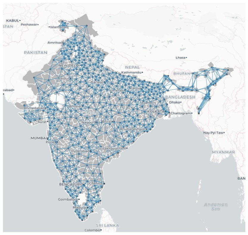
A formal analysis of spatial dependence requires the neighborhood of each district, which the 6NN weight matrix described above supplies. Figure 5 visualizes that connectivity as a network, in which each node represents a district centroid and each edge connects a district to one of its six nearest neighbors.

In [3]:

# Plot the spatial weights matrix
# This will visualize the spatial relationships between observations defined by the weights matrix W
fig, ax = plt.subplots(ncols=1, nrows=1, figsize=(14,10))
plot_spatial_weights(W, gdf, indexed_on='Census_no', ax=ax)
cx.add_basemap(ax, crs=gdf.crs.to_string(), source=cx.providers.CartoDB.Positron, attribution=False)
cx.add_basemap(ax, crs=gdf.crs.to_string(), source=cx.providers.CartoDB.PositronOnlyLabels, attribution=False)
ax.set_axis_off()
plt.show()

Figure 5: Spatial connectivity structure based on six nearest neighbors
Notes: Each node represents a district centroid. Each edge connects a district to one of its six geographically closest neighbors. The weight matrix is row-standardized.
Source: Data from Chanda and Kabiraj (2020). See Spatial dependence notebook for source code.

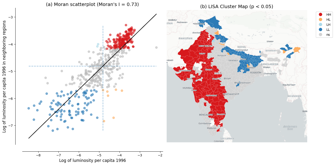
Spatial dependence can be understood through two complementary concepts: the overall degree of clustering in the data, and the specific locations of statistically significant clusters and spatial outliers. The Global Moran’s I statistic captures the first of these concepts. In our data, the Moran’s I for initial luminosity per capita is 0.73 (\(p = 0.001\)), which indicates strong positive spatial autocorrelation: districts with high (low) initial luminosity tend to be surrounded by districts that are also bright (dim). 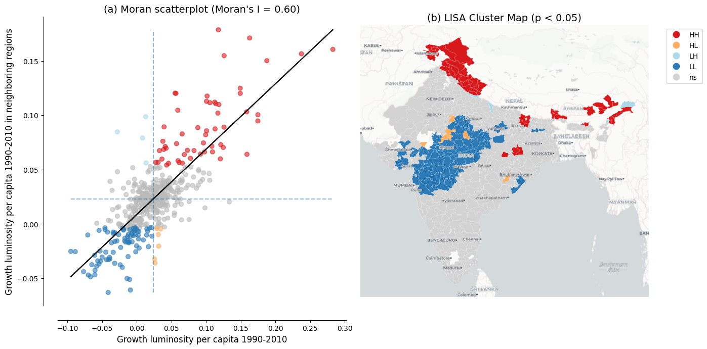The Moran’s I for luminosity growth is 0.60 (\(p = 0.001\)), which confirms that the growth rates of neighboring districts are also significantly correlated.

We now turn to the LISA statistics, which locate the significant clusters and outliers behind these global measures. Figure 6 presents the Moran scatterplot and LISA cluster map for initial luminosity per capita. HH clusters mark the most luminous regions and their bright neighbors, while LL clusters highlight contiguous areas of low luminosity. These are predominantly in eastern and northern India, in Bihar, eastern Uttar Pradesh, and Jharkhand, together with the Himalayan north and the northeast.

In [4]:

# Initialize the subplots
f, ax = plt.subplots(1, 2, figsize=(14, 7))

# 1. Plot Moran Scatterplot and customize labels
moran_scatterplot(moranLocal, p=0.05, zstandard=False, aspect_equal=f, ax=ax[0])
ax[0].set_title(f"(a) Moran scatterplot (Moran's I = {moranI1})", fontsize=14)
ax[0].set_xlabel("Log of luminosity per capita 1996", fontsize=12)
ax[0].set_ylabel("Log of luminosity per capita 1996 in neighboring regions", fontsize=12)

# 2. Plot LISA Cluster map and customize title
lisa_cluster(moranLocal, gdf, p=0.05, 
             legend_kwds={'bbox_to_anchor':(1.05, 1), 'loc': 'upper left'}, 
             ax=ax[1])
ax[1].set_title("(b) LISA Cluster Map (p < 0.05)", fontsize=14)

# 3. Add basemap to the cluster map
cx.add_basemap(ax[1], 
               crs=gdf.crs.to_string(), 
               source=cx.providers.CartoDB.Positron, 
               attribution=False)

# Optional: Remove axes ticks for the map to make it cleaner
ax[1].set_axis_off()

plt.tight_layout()
try:
    plt.savefig("../images/lisaMAP1.png", dpi=150, bbox_inches='tight')
except OSError:
    pass  # Skip file export when running in Colab
plt.show()

Figure 6: Spatial dependence in the initial level of luminosity
Notes: Panel (a) shows the Moran scatterplot with Global Moran’s I statistic. Panel (b) shows the LISA cluster map with statistically significant clusters at p < 0.05 based on 999 permutations.
Source: Data from Chanda and Kabiraj (2020). See Spatial dependence notebook for source code.

The same analysis applied to luminosity growth rates reveals a pattern that is largely the inverse of the initial clusters, as Figure 7 shows. No district that formed an HH cluster in initial luminosity forms one in luminosity growth: some appear instead as LL clusters, and most lose significance. Part of the initially dimmest cluster, in turn, emerges as an HH cluster in growth. That inversion is the spatial signature of the convergence process, and it motivates the use of spatial econometric methods.

In [5]:

# Initialize the subplots
f, ax = plt.subplots(1, 2, figsize=(14, 7))

# 1. Plot Moran Scatterplot and customize labels
moran_scatterplot(moranLocal2, p=0.05, zstandard=False, aspect_equal=f, ax=ax[0])
ax[0].set_title(f"(a) Moran scatterplot (Moran's I = {moranI2})", fontsize=14)
ax[0].set_xlabel("Growth luminosity per capita 1996-2010", fontsize=12)
ax[0].set_ylabel("Growth luminosity per capita 1996-2010 in neighboring regions", fontsize=12)

# 2. Plot LISA Cluster map and customize title
lisa_cluster(moranLocal2, gdf, p=0.05, 
             legend_kwds={'bbox_to_anchor':(1.05, 1), 'loc': 'upper left'}, 
             ax=ax[1])
ax[1].set_title("(b) LISA Cluster Map (p < 0.05)", fontsize=14)

# 3. Add basemap to the cluster map
cx.add_basemap(ax[1], 
               crs=gdf.crs.to_string(), 
               source=cx.providers.CartoDB.Positron, 
               attribution=False)

# Optional: Remove axes ticks for the map to make it cleaner
ax[1].set_axis_off()

plt.tight_layout()
try:
    plt.savefig("../images/lisaMAP2.png", dpi=150, bbox_inches='tight')
except OSError:
    pass  # Skip file export when running in Colab
plt.show()

Figure 7: Spatial dependence in the growth rate of luminosity
Notes: Panel (a) shows the Moran scatterplot with Global Moran’s I statistic. Panel (b) shows the LISA cluster map with statistically significant clusters at p < 0.05 based on 999 permutations.
Source: Data from Chanda and Kabiraj (2020). See Spatial dependence notebook for source code.

3.3 Evidence of spatial spillovers in regional convergence

The regression results of Table 2 provide evidence of both unconditional and conditional convergence across districts in India, under ordinary least squares (OLS) and under the spatial specifications alike. The direct effects, which represent within-district convergence, remain negative and of similar order across specifications, ranging from -0.020 to -0.026. This consistency across specifications and estimation methods suggests that poorer districts are catching up to their wealthier counterparts, even after controlling for district characteristics and state-level fixed effects.

In [6]:

from IPython.display import Markdown

cols = ["Model 1", "Model 2", "Model 3", "Model 4"]


# A real minus (U+2212), not the ASCII hyphen. LaTeX treats a hyphen as a legal
# line-break point, which in a narrow table column strands the sign on its own
# line; U+2212 cannot break, and it is the correct glyph for a negative number.
MINUS = "\u2212"


def _num(x, nd=3):
    return "{:.{}f}".format(x, nd).replace("-", MINUS)


def _est(est, se):
    return "{}{}".format(_num(est), stars(est, se))


def _se(se):
    return "({})".format(_num(se))


lines = [
    "|          | Model 1 |       | Model 2 |         | Model 3 |       | Model 4 |         |",
    # Uniform dash counts: pandoc derives the LaTeX column widths from this row,
    # and uneven counts gave two columns a narrower width than their contents.
    "|---------|---------|---------|---------|---------|---------|---------|---------|---------|",
    "|          | OLS     | SDM   | OLS     | SDM     | OLS     | SDM   | OLS     | SDM     |",
]

# Direct effect (+ SE row)
row, se_row = "| Direct   |", "|          |"
for c in cols:
    o, s = results[c]["ols"], results[c]["sdm"]
    row += " {} | {} |".format(_est(o["direct"], o["direct_se"]), _est(s["direct"], s["direct_se"]))
    se_row += " {} | {} |".format(_se(o["direct_se"]), _se(s["direct_se"]))
lines += [row, se_row]

# Indirect effect (OLS = --, no SE; + SE row for SDM)
row, se_row = "| Indirect |", "|          |"
for c in cols:
    s = results[c]["sdm"]
    row += " -- | {} |".format(_est(s["indirect"], s["indirect_se"]))
    se_row += "  | {} |".format(_se(s["indirect_se"]))
lines += [row, se_row]

# Total effect (+ SE row)
row, se_row = "| Total    |", "|          |"
for c in cols:
    o, s = results[c]["ols"], results[c]["sdm"]
    row += " {} | {} |".format(_est(o["total"], o["total_se"]), _est(s["total"], s["total_se"]))
    se_row += " {} | {} |".format(_se(o["total_se"]), _se(s["total_se"]))
lines += [row, se_row]

# Controls / State FE / AIC
ctrl, fe_row, aic = "| Controls |", "| State FE |", "| AIC      |"
for c in cols:
    ctrl += " {0} | {0} |".format(results[c]["controls"])
    fe_row += " {0} | {0} |".format(results[c]["fe"])
    aic += " {} | {} |".format(_num(results[c]["ols"]["aic"], 0), _num(results[c]["sdm"]["aic"], 0))
lines += [ctrl, fe_row, aic]

Markdown("\n".join(lines))

In [7]:

Table 2: Unconditional and conditional convergence across districts. Heteroskedasticity-robust (HC1) standard errors for OLS and Monte-Carlo standard errors for the SDM impacts in parentheses. *** p < 0.01, ** p < 0.05, * p < 0.10.

	Model 1		Model 2		Model 3		Model 4
	OLS	SDM	OLS	SDM	OLS	SDM	OLS	SDM
Direct	−0.020***	−0.021***	−0.022***	−0.021***	−0.025***	−0.026***	−0.025***	−0.025***
	(0.002)	(0.002)	(0.003)	(0.002)	(0.003)	(0.002)	(0.003)	(0.002)
Indirect	–	−0.001	–	−0.001	–	−0.015*	–	−0.012*
		(0.006)		(0.005)		(0.008)		(0.007)
Total	−0.020***	−0.022***	−0.022***	−0.022***	−0.025***	−0.041***	−0.025***	−0.037***
	(0.002)	(0.006)	(0.003)	(0.005)	(0.003)	(0.009)	(0.003)	(0.007)
Controls	No	No	No	No	Yes	Yes	Yes	Yes
State FE	No	No	Yes	Yes	No	No	Yes	Yes
AIC	−1945	−2292	−2409	−2468	−2211	−2358	−2465	−2501

In the OLS specifications, the direct effect is -0.020 in Model 1 and -0.022 in Model 2, and it strengthens to -0.025 once district characteristics are added in Models 3 and 4. Omitting these characteristics therefore attenuates the estimated speed of convergence, and the spatial Durbin direct effects match this pattern in the conditional models, at -0.026 in Model 3 and -0.025 in Model 4. State fixed effects absorb unobserved state-level heterogeneity, such as differences in governance and institutional quality, which tightens the standard errors on the spatial impacts and moderates the spatial total effect rather than strengthening it further.

The spatial Durbin model also reveals spillover effects that OLS does not capture, and these indirect effects, which measure the influence of the initial conditions of neighboring districts on the growth rate of a district, follow a notable pattern across specifications. In the unconditional models (Models 1 and 2), the estimated indirect effects are negative but small and statistically insignificant, at -0.001 in both.¹¹ Once district-level controls are introduced (Models 3 and 4), the indirect effects become both larger in magnitude and statistically significant at the 10% level, reaching -0.015 in Model 3 and -0.012 in our most comprehensive Model 4. The spatial channels of convergence therefore become discernible only after accounting for district-specific characteristics.

The total impact of initial conditions on growth, combining both direct and spillover effects, is substantially larger when we account for spatial dependence. In our fully specified model (Model 4), the total convergence effect in the spatial Durbin model (-0.037) is approximately 51% larger in magnitude than the OLS estimate (-0.025). Translated into an annual speed of convergence, this raises the implied speed from about 3.0% under OLS to about 5.2% under the SDM, and it shortens the implied half-life from roughly 23 to 13 years. The gap is even larger in Model 3 (SDM total -0.041 against OLS -0.025, or 67%), but the Model 3 and Model 4 spillover estimates are statistically indistinguishable, so we anchor our interpretation on the preferred Model 4. These differences indicate that in this setting conventional non-spatial approaches understate the speed of regional convergence by failing to capture the additional convergence channels created through spatial spillovers.

In [8]:

T = 14  # 1996-2010; dependent variable is the average annual growth rate


def _speed(beta):
    arg = 1 + beta * T
    if arg <= 0:
        return float("nan"), float("nan")
    lam = -np.log(arg) / T
    return lam, np.log(2) / lam


srows = [
    "| Model | OLS speed | SDM speed | OLS half-life | SDM half-life |",
    "|-------|-----------|-----------|---------------|---------------|",
]
for c in ["Model 1", "Model 2", "Model 3", "Model 4"]:
    lo, hlo = _speed(results[c]["ols"]["total"])
    ls, hls = _speed(results[c]["sdm"]["total"])
    srows.append("| {} | {:.1%} | {:.1%} | {:.0f} yr | {:.0f} yr |".format(c, lo, ls, hlo, hls))
Markdown("\n".join(srows))

In [9]:

Table 3: Implied annual speed of convergence and half-life by model, from the OLS and SDM total effects of initial luminosity.

Model	OLS speed	SDM speed	OLS half-life	SDM half-life
Model 1	2.3%	2.6%	30 yr	27 yr
Model 2	2.6%	2.7%	27 yr	26 yr
Model 3	3.0%	6.2%	23 yr	11 yr
Model 4	3.0%	5.2%	23 yr	13 yr

Table 3 reports the implied speeds and half-lives for all four specifications. The spatial premium is concentrated in the conditional models. In Models 1 and 2 the OLS and SDM speeds are nearly identical, whereas in Models 3 and 4 the SDM raises the implied speed from 3.0% to 6.2% and 5.2%, shortening the half-life from 23 years to 11 and 13 years respectively.¹²

The Akaike Information Criterion (AIC) consistently favors the spatial Durbin model over OLS across all four specifications, and the most comprehensive model (Model 4 SDM) achieves the lowest AIC value of -2501 compared to -2465 for the corresponding OLS.¹³ These results suggest that regional convergence in India operates not only through district-specific factors but also through spatial interactions between neighboring districts, so that ignoring those interactions yields both underestimated convergence speeds and inferior model performance.

A word of caution is in order about how the indirect effects should be read. The spatial Durbin model identifies spatial dependence in reduced form: it establishes that the growth of a district covaries with the initial conditions of its neighbors, conditional on its own characteristics, but it does not establish why. Several distinct processes generate the same reduced-form pattern, since neighboring districts share geographic and agro-climatic conditions, are often governed by the same state and so inherit common institutional and policy environments that our state fixed effects absorb only in part, are connected by infrastructure whose effects do not stop at administrative boundaries, and are exposed to any omitted determinant of growth that is itself spatially clustered. The measurement issues discussed below point in the same direction, since blooming spreads light across district boundaries and can raise the apparent correlation between neighbors for reasons unrelated to economic interaction. We therefore read the indirect effects as evidence that spatial structure is a feature of the convergence process, and not as an estimate of the causal effect of the conditions of one district on the growth of another. Establishing which channels are at work, and whether they are causal, would require research designs built for that purpose, a point we return to in the discussion.

3.4 How these estimates compare with the convergence literature

The speeds reported above can be placed against three benchmarks. The first is other work on Indian districts using the same proxy. Beyer and Yamada (2020) report 2.4% absolute and 3.7% conditional convergence for India over 2013–2019, against our own 2.3% and 3.0%. That two independent applications of the same measurement strategy recover similar non-spatial rates, despite different periods and different generations of the sensor, is reassuring about the proxy.

The second benchmark is convergence measured from luminosity elsewhere. Basher, Rashid, and Uddin (2023) find absolute convergence of 4.57% per year across the 64 districts of Bangladesh, roughly double the 2.3% we obtain on the same unconditional basis. Carrington and Jiménez-Ayora (2021) report a speed near 2% for Ecuadorian provinces, and Kacou (2022) finds multiple equilibria across 49 African countries. Our own unconditional non-spatial estimate therefore sits near the familiar 2% regularity, while the conditional spatial estimates lie well above it.¹⁴ A meta-analysis of some 600 published estimates nevertheless warns against treating that regularity as a law (Abreu, de Groot, and Florax 2005). These comparisons locate our estimates rather than validate them.

The third benchmark bears most directly on what this article adds. That convergence estimates are sensitive to spatial dependence is established, but the direction of the adjustment is not. Our own rise from 3.0% to 5.2% agrees with Diop (2018), who concludes that non-spatial estimates may be considerably understated. Others find the opposite: lower speeds for European regions (Isla-Castillo, Garashchuk, and Podadera-Rivera 2024), neighbor effects that slow convergence across Indonesian districts (Santos-Marquez, Gunawan, and Mendez 2022), and divergence rather than convergence across Indian states (Lolayekar and Mukhopadhyay 2019). The substantive point is therefore not that spatial dependence matters, which is already known, but that here it works in the direction of faster measured convergence, and that the scale of analysis is part of what determines the answer.¹⁵

3.5 Robustness to alternative spatial weight matrices

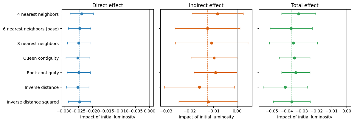
The spillover results above use the 6NN spatial weight matrix defined in Section 2. To assess their sensitivity to this choice, we re-estimate the preferred Model 4 under six alternative specifications and compare them with the 6NN baseline. The alternatives are four- and eight-nearest neighbors, queen and rook contiguity, and inverse distance and inverse-distance-squared, the last two applied within a distance band.

In [10]:

names = [n for n, _ in WMATS]
ypos = np.arange(len(names))[::-1]   # top-to-bottom in listed order
effects = [("direct", "Direct", "#2c7fb8"), ("indirect", "Indirect", "#d95f0e"), ("total", "Total", "#31a354")]

fig, axes = plt.subplots(1, 3, figsize=(12, 4.2), sharey=True)
for ax, (key, label, color) in zip(axes, effects):
    est = np.array([res[n][key] for n in names])
    se = np.array([res[n][key + "_se"] for n in names])
    ax.errorbar(est, ypos, xerr=1.96 * se, fmt="o", color=color, ecolor=color,
                elinewidth=1.5, capsize=3, markersize=6)
    ax.axvline(0, color="0.6", lw=0.8)
    base = res["6 nearest neighbors (base)"][key]
    ax.axvline(base, color=color, ls="--", lw=1.0, alpha=0.7)
    ax.set_title("{} effect".format(label))
    ax.set_xlabel("Impact of initial luminosity")
axes[0].set_yticks(ypos)
axes[0].set_yticklabels(names)
fig.tight_layout()
plt.show()

Figure 8: Robustness of the Model 4 spatial impacts of initial luminosity to the choice of spatial weight matrix. Points are Direct, Indirect, and Total impacts; bars are 95% Monte-Carlo confidence intervals. The dashed lines mark the 6NN baseline estimates.

In [11]:

from IPython.display import Markdown


# A real minus (U+2212), not the ASCII hyphen: LaTeX may break a line at a
# hyphen, which strands the sign on its own line in a narrow table column.
MINUS = "\u2212"


def _num(x, nd=3):
    return "{:.{}f}".format(x, nd).replace("-", MINUS)


def _cell(est, se):
    return "{}{}".format(_num(est), stars(est, se))


def _se(se):
    return "({})".format(_num(se))


# Standard errors go on their own row rather than in a <br> inside the cell:
# pandoc drops <br> when it writes LaTeX, which concatenated the estimate and
# its standard error into one over-wide cell. This also matches tbl-models.
rows = [
    "| Weight matrix | Direct | Indirect | Total | AIC |",
    "|---------------|--------|----------|-------|-----|",
]
for name, _ in WMATS:
    r = res[name]
    rows.append("| {} | {} | {} | {} | {} |".format(
        name,
        _cell(r["direct"], r["direct_se"]),
        _cell(r["indirect"], r["indirect_se"]),
        _cell(r["total"], r["total_se"]),
        _num(r["aic"], 0),
    ))
    rows.append("| | {} | {} | {} | |".format(
        _se(r["direct_se"]), _se(r["indirect_se"]), _se(r["total_se"]),
    ))
Markdown("\n".join(rows))

In [12]:

Table 4: Model 4 spatial impacts of initial luminosity under alternative spatial weight matrices (full LeSage–Pace method; Monte-Carlo standard errors in parentheses). *** p < 0.01, ** p < 0.05, * p < 0.10.

Weight matrix	Direct	Indirect	Total	AIC
4 nearest neighbors	−0.024***	−0.008	−0.032***	−2468
	(0.002)	(0.005)	(0.006)
6 nearest neighbors (base)	−0.025***	−0.012*	−0.037***	−2501
	(0.002)	(0.007)	(0.007)
8 nearest neighbors	−0.025***	−0.011	−0.036***	−2485
	(0.002)	(0.008)	(0.008)
Queen contiguity	−0.025***	−0.010**	−0.035***	−2463
	(0.002)	(0.005)	(0.005)
Rook contiguity	−0.025***	−0.009**	−0.034***	−2469
	(0.002)	(0.004)	(0.005)
Inverse distance	−0.025***	−0.016**	−0.041***	−2486
	(0.002)	(0.007)	(0.008)
Inverse distance squared	−0.025***	−0.012*	−0.037***	−2485
	(0.002)	(0.006)	(0.006)

The direct and total convergence effects are robust to the choice of spatial weights, and the spillover component is consistently negative but more sensitive (Figure 8 and Table 4). The direct (within-district) convergence effect is essentially unchanged across all seven specifications, ranging from -0.024 to -0.025 and always significant at the 1% level. The total convergence effect likewise remains negative and significant throughout, ranging from -0.032 to -0.041, with the 6NN baseline (-0.037) near the middle of this range. The indirect (spillover) component is negative in every specification and statistically significant under five of the seven, which is a consistent if weaker pattern. This stability indicates that the direct and total convergence effects are not an artifact of the particular neighbor definition.

The results reported so far treat luminosity as a proxy for economic output, which is the use that the convergence literature has made of it. The discussion that follows asks first what the magnitude of these estimates implies for regional policy, and what rests on the use of a single growth period. It then turns to a second use of the same data, since nighttime lights also record electrification, urbanization, and broader socioeconomic conditions, and the reproducible workflow assembled here can be pointed at those dimensions as readily as at output. That possibility is pursued in an exploratory way, asking how luminosity relates to cultural participation across Indian states.

4 Discussion

4.1 What the magnitude of the effects implies for regional policy

The difference between the two readings of Model 4 is large enough to matter for policy. Under the OLS estimate, a district closes half of the gap to its steady state in about 23 years; under the spatial Durbin estimate, in about 13 years. Over the fourteen years of our sample, that is the difference between closing roughly 34% and roughly 52% of the initial gap. The first figure describes catch-up over a generation; the second, catch-up within the horizon over which development programs are designed, funded, and evaluated. Under the faster rate, the returns to well-targeted support should appear within a normal evaluation window.

The results also speak to the level at which such policies should operate. We find convergence across districts over 1996–2010, whereas Lolayekar and Mukhopadhyay (2019), working with Indian states over a longer period, find divergence. Catch-up visible at the district level and absent at the state level is consistent with the district being the more informative unit of intervention, which the Aspirational Districts Programme of India already assumes.¹⁶ The spatial results add a qualification, since a lagging district surrounded by other lagging districts is in a different position from one adjacent to a growing cluster. A targeting rule that ranks districts one at a time will not register that difference.

Spillovers cut both ways, however, and the Indian evidence on place-based policy is a caution as much as an encouragement. Hasan, Jiang, and Rafols (2021) find that a tax exemption for industrially backward districts raised firm entry and employment partly by displacing activity from neighboring districts that narrowly missed qualifying, with effects that did not outlast the program. Displacement of that kind would appear in our framework as a spatial relationship between neighbors, which is not a spillover on which coordinated regional policy can be built. What the satellite record does support is measurement.¹⁷ The readings above therefore hold only if the indirect effects reflect genuine interaction between districts, and the reduced-form evidence is consistent with that but does not establish it.

4.2 The single growth period and what a panel would require

The estimates reported above rest on a single growth period, and the cost of that design should be stated plainly. One long difference cannot trace how convergence evolved within the period, cannot show whether the spatial spillovers were stronger in some years than in others, and cannot separate long-run convergence from what was specific to these fourteen years, which in India included the maturing of the post-1991 reforms. Examining those dynamics lies beyond an article that adds a spatial dimension to an existing cross-sectional result. The immediate obstacle is in any case the data, since district population is observed only at the decennial censuses.¹⁸ Interpolated denominators touch only the endpoints of a long difference, whereas in a panel they would enter every observation, and would do so in the time dimension that a panel exists to exploit.

What such a panel would be worth is the more interesting question, and here two problems compound. The first predates nighttime lights: panel estimates of convergence run far above cross-sectional ones, and Caselli, Esquivel, and Lefort (1996) obtain a rate near 10% per year against the 2% that cross-sections deliver.¹⁹ How that gap should be read remains contested, so a panel would give not a better-identified version of our estimate but an estimate of something different. The second problem is specific to the proxy, since luminosity discriminates differences across places far better than changes over time (X. Chen and Nordhaus 2019; Asher et al. 2021), and over short intervals the ratio of signal to measurement error falls sharply.²⁰ The periods compared should therefore be long, and harmonized DMSP–VIIRS series now make a sequence of non-overlapping long differences feasible across roughly three decades (Li et al. 2020), which is the most promising temporal extension of this work.

4.3 An exploratory extension: Luminosity and cultural participation

Nighttime lights capture not just GDP but a composite of electrification, urbanization, infrastructure, and broader socioeconomic conditions (Henderson, Storeygard, and Weil 2012; Mellander et al. 2015). In this section, we examine the association between luminosity and cultural participation patterns across Indian states.

A growing literature argues that regional cultural attitudes constitute an independent factor in economic development, not merely a by-product of income or institutions. In particular, Tubadji (2025) applies the Culture-Based Development framework, whose central claim is a directional one. Cultural attitudes and the participation patterns that reveal them are treated as a factor shaping local development, rather than as an outcome that development produces. That direction also marks the limit of what the exercise below can establish.²¹

For India, the National Sample Survey (NSS) 47th Round (July–December 1991) surveys household cultural participation, and nighttime lights for the adjacent year 1992 are available for 32 states and union territories. Following the Culture-Based Development framework, we reduce these survey items to six dimensions and aggregate them to state means.²² This part of the analysis uses the Consistent and Corrected Nighttime Lights series rather than the radiance-calibrated composites used above, because it is the product that covers 1992. Given the small sample (\(N\) = 32) and the leverage that small territories at the extremes of the distribution exert on linear correlation measures, we report Spearman rank correlations throughout. 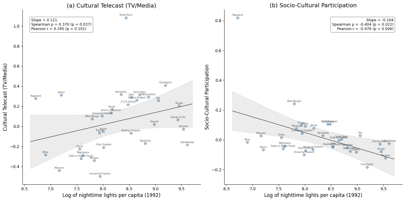Figure 9 presents the relationship between log nighttime lights per capita and the two cultural dimensions that show statistically significant associations.

In [13]:

# Key variables for the core message
key_vars = ["LC_Telecast", "SC"]
key_labels = {
    "LC_Telecast": "Cultural Telecast (TV/Media)",
    "SC": "Socio-Cultural Participation",
}
panel_titles = ["(a) Cultural Telecast (TV/Media)", "(b) Socio-Cultural Participation"]

fig, axes = plt.subplots(1, 2, figsize=(14, 7))

for i, var in enumerate(key_vars):
    ax = axes[i]
    x = gdf["ln_ntl_pc"]
    y = gdf[var]

    # Scatter points (steelblue to match manuscript style)
    ax.scatter(x, y, s=45, alpha=0.5, color="steelblue", edgecolors="black", linewidth=0.3, zorder=5)

    # Regression line with confidence band
    slope, intercept, r_val, p_val, se = stats.linregress(x, y)
    x_line = np.linspace(x.min() - 0.1, x.max() + 0.1, 200)
    y_line = intercept + slope * x_line
    ax.plot(x_line, y_line, color="black", linewidth=0.8, zorder=4)

    # Confidence band (95%)
    n = len(x)
    x_mean = x.mean()
    se_fit = np.sqrt(((y - (intercept + slope * x))**2).sum() / (n - 2)) * \
             np.sqrt(1/n + (x_line - x_mean)**2 / ((x - x_mean)**2).sum())
    t_crit = stats.t.ppf(0.975, n - 2)
    ax.fill_between(x_line, y_line - t_crit * se_fit, y_line + t_crit * se_fit,
                    alpha=0.15, color="gray", zorder=3)

    # Label each state
    for _, row in gdf.iterrows():
        ax.annotate(
            row["region"], (row["ln_ntl_pc"], row[var]),
            fontsize=5.5, alpha=0.65, ha="center", va="bottom",
            xytext=(0, 3), textcoords="offset points",
        )

    # Spearman correlation
    rho, p_spearman = stats.spearmanr(x, y)

    # Annotation box (top-left or top-right depending on slope sign)
    box_x = 0.95 if slope < 0 else 0.05
    box_ha = "right" if slope < 0 else "left"
    ax.annotate(
        f"Slope = {slope:.3f}\n"
        f"Spearman \u03c1 = {rho:.3f} (p = {p_spearman:.3f})\n"
        f"Pearson r = {r_val:.3f} (p = {p_val:.3f})",
        xy=(box_x, 0.95), xycoords="axes fraction",
        fontsize=9, ha=box_ha, va="top",
        bbox=dict(boxstyle="round,pad=0.4", facecolor="white", edgecolor="gray", alpha=0.85),
    )

    ax.set_title(panel_titles[i], fontsize=14)
    ax.set_xlabel("Log of nighttime lights per capita (1992)", fontsize=12)
    ax.set_ylabel(key_labels[var], fontsize=12)

    # Minimal style
    ax.spines["top"].set_visible(False)
    ax.spines["right"].set_visible(False)
    ax.tick_params(labelsize=10)

plt.tight_layout()
plt.show()

Figure 9: Relationship between nightlight luminosity and cultural participation across 32 Indian states
Notes: Each point represents one of the 32 Indian states and union territories. Panel (a) shows the bivariate relationship between log nighttime lights per capita and cultural telecast (TV/media); Panel (b) shows the relationship with socio-cultural participation. Solid line is the OLS regression; gray band shows the 95% confidence interval (t-distribution, 30 df). Annotations report regression slope, Spearman rank correlation, and Pearson correlation.
Source: Nighttime lights from CCNL DMSP-OLS (Zhao et al., 2022). Cultural participation from NSS 47th Round (July–December 1991). See Spatial culture notebook for source code.

Cultural telecast (TV/media) is positively associated with luminosity, with a Spearman rank correlation of 0.370 (\(p = 0.037\)), so more luminous states tend to rank higher on that dimension. Socio-cultural participation, in contrast, is negatively associated, with a Spearman rank correlation of \(-0.404\) (\(p = 0.022\)), so less luminous states tend to rank higher on it. We refer to these two dimensions as media-based cultural consumption and community-based participation, respectively. This suggests that less urbanized regions rely more on collective, in-person forms of cultural participation than on media infrastructure.

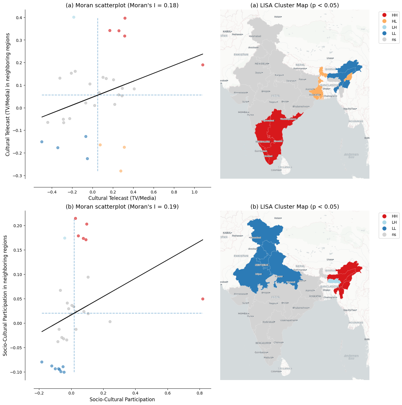
Figure 10 maps the spatial distribution of the two cultural variables through the lens of a LISA analysis. The Low-Low cluster of media-based cultural consumption in the northeast coincides with the Low-Low cluster in the nighttime lights data, whereas the High-High clusters do not coincide: media-based cultural consumption forms one in the southern states, and community-based participation forms one in the northeast. The remaining four cultural dimensions show no statistically significant association with luminosity, and these findings rest on a small cross-section of 32 states observed at a single point in time, so larger datasets covering more regions and periods would be needed to establish whether the patterns are robust.

In [14]:

# Reproject to Web Mercator for basemap overlay
gdf_wm = gdf.to_crs(epsg=3857)

# Two key cultural variables only
lisa_vars = ["LC_Telecast", "SC"]
lisa_labels = {
    "LC_Telecast": "Cultural Telecast (TV/Media)",
    "SC": "Socio-Cultural Participation",
}
panel_rows = ["(a)", "(b)"]

# Compute LISA for each variable
lisa_objects = {}
moran_globals = {}
for var in lisa_vars:
    lisa_objects[var] = Moran_Local(gdf_wm[var].values, W, permutations=999, seed=12345)
    moran_globals[var] = Moran(gdf_wm[var].values, W, permutations=999)

# Create 2-row x 2-column figure
fig, axes = plt.subplots(2, 2, figsize=(14, 14))

for i, var in enumerate(lisa_vars):
    moranI = f"{moran_globals[var].I:.2f}"

    # Left panel: Moran scatterplot
    moran_scatterplot(lisa_objects[var], p=0.05, zstandard=False, aspect_equal=False, ax=axes[i, 0])
    axes[i, 0].set_title(
        f"{panel_rows[i]} Moran scatterplot (Moran's I = {moranI})", fontsize=14
    )
    axes[i, 0].set_xlabel(lisa_labels[var], fontsize=12)
    axes[i, 0].set_ylabel(f"{lisa_labels[var]} in neighboring regions", fontsize=12)
    axes[i, 0].tick_params(labelsize=10)

    # Right panel: LISA cluster map
    lisa_cluster(
        lisa_objects[var], gdf_wm, p=0.05,
        legend_kwds={"bbox_to_anchor": (1.05, 1), "loc": "upper left"},
        ax=axes[i, 1],
    )
    axes[i, 1].set_title(
        f"{panel_rows[i]} LISA Cluster Map (p < 0.05)", fontsize=14
    )

    # Add CartoDB basemap (matching manuscript style)
    cx.add_basemap(
        axes[i, 1], crs=gdf_wm.crs.to_string(),
        source=cx.providers.CartoDB.Positron, attribution=False,
    )
    cx.add_basemap(
        axes[i, 1], crs=gdf_wm.crs.to_string(),
        source=cx.providers.CartoDB.PositronOnlyLabels, attribution=False,
    )
    axes[i, 1].set_axis_off()

plt.tight_layout()
plt.show()

Figure 10: LISA cluster maps of cultural participation across 32 Indian states
Notes: Panel (a) shows results for cultural telecast (TV/media); Panel (b) for socio-cultural participation. Left subpanels show Moran scatterplots with the Global Moran’s I statistic. Right subpanels show LISA cluster maps with statistically significant clusters at p < 0.05 based on 999 permutations and a 6-nearest-neighbors spatial weights matrix. Region labels are overlaid from the CartoDB Positron basemap.
Source: Cultural participation data from NSS 47th Round (July–December 1991). See Spatial culture notebook for source code.

Two connections to the main analysis are worth drawing out, both offered as interpretation rather than as findings. The first concerns what luminosity measures. A positive association with media-based cultural consumption and a negative one with community-based participation are what one would expect if luminosity tracks electrification and urbanization rather than economic output alone. The cultural results are, in that sense, a small piece of evidence about the composite nature of the proxy on which the convergence analysis rests, and they bear on the measurement issues discussed below.

The second connection concerns spatial structure. Cultural participation is not distributed randomly across states, since both dimensions examined here are significantly spatially autocorrelated. Factors of this kind, spatially clustered and correlated with development, are precisely what a spatial Durbin model absorbs into its indirect effects when they are not measured directly. We cannot test this with state-level data for a single adjacent period, and we do not claim that cultural participation drives the spillovers estimated in the results section. What the exercise does is make concrete what a reduced-form spatial model may be capturing, and it suggests that the Culture-Based Development framework offers one route to testing the question directly, should comparable data become available at the district level and over time.

4.4 New research directions

Three kinds of gap limit what this literature can currently establish: the data themselves, the geography they cover, and the theories they have been used to test. The first is well documented, since the radiance-calibrated DMSP-OLS series we adopt from Chanda and Kabiraj (2020), and on which this literature rests (Henderson, Storeygard, and Weil 2012; X. Chen and Nordhaus 2011), is top-coded in bright urban cores, uncalibrated on board, and blurred across boundaries by blooming (Gibson et al. 2021; Abrahams, Oram, and Lozano-Gracia 2018). Top-coding leaves the net bias in our convergence coefficient ambiguous in sign, while blooming raises the apparent correlation between neighbors and therefore bears directly on the spillover estimates.²³ The Visible Infrared Imaging Radiometer Suite (VIIRS) and harmonized DMSP–VIIRS series address all three problems (Elvidge et al. 2017; Li et al. 2020; Chiovelli et al. 2026), and multi-source methods improve measurement where lights alone are weak.²⁴ Re-estimating our specification on those data is the most immediate extension of the analysis reported here.

The second gap concerns geography, and it is not that some regions have gone unstudied. A single instrument observes the whole planet under a common protocol, which makes measurements comparable in a way that national accounts are not (Henderson, Storeygard, and Weil 2012), but what it records is light rather than economic activity. Roughly one fifth of the settlement footprint of the planet emits no detectable radiance, and unlit settlements are concentrated in Africa (McCallum et al. 2022). Africa is nonetheless well covered by this literature (Kacou 2022), as are China (Glawe and Mendez 2025), Indonesia (Miranti and Mendez 2023), Thailand (Tipayalai and Mendez 2024), and Turkey (Ursavaş and Mendez 2023). The real gap is that the places where lights carry least information, rural and sparsely electrified areas, are the places where administrative statistics are weakest and a satellite proxy would be most valuable.²⁵ Closing it calls less for further applications of the same proxy than for validation against ground data in those settings.

The third gap concerns theory, since luminosity is now applied well beyond the question asked here. Within convergence analysis, our framework yields an average effect rather than heterogeneity across the distribution, and it captures spillovers in reduced form, gaps that distribution dynamics and quasi-experimental designs such as that of Asher and Novosad (2020) are built to fill.²⁶ Beyond convergence, lights now serve the study of city size (Ch, Martin, and Vargas 2021), electrification and the provision of public goods (Min et al. 2013), armed conflict (Witmer and O’Loughlin 2011), the cultural participation theorized by Tubadji (2025), and the local effect of policies and shocks at fine spatial scales (Bluhm and McCord 2022). One caveat governs all of these uses: lights discriminate differences across places far better than changes over time, so evaluations over short horizons require validation against local ground data.²⁷ The design used here, a fourteen-year horizon, rests mostly on cross-sectional variation, which is what lights currently support best.

Taken together, these three gaps describe a research agenda rather than a list of caveats, and none of the work they imply requires starting from scratch. The pipeline behind this article is public, documented, and executable in a browser, so a reader can open the relevant notebook, substitute data from another country or a later period, and re-run it. That is the contribution we would most like this article to make: not an estimate of how quickly Indian districts converged between 1996 and 2010 alone, but a working template that lowers the cost of asking the same question elsewhere.

4.5 Research reproducibility and open science

As Donaldson and Storeygard (2016) note, methodological choices in processing remotely sensed data, such as sensor inter-calibration, can affect the empirical conclusions. The same applies further down our own pipeline, at the construction of the spatial weight matrix. Our own robustness analysis is a case in point: the estimated convergence effects survive seven definitions of the neighborhood, but that is something a reader can only confirm because the code that produced each of them is available.

Open-source tools and cloud platforms lower the barriers to that kind of verification, and cloud-based notebooks for processing nighttime lights remove the need for specialized local software (Patnaik and Mendez 2024). Open data, version-controlled code, and cloud execution together make the full pipeline, from satellite imagery to econometric results, verifiable and extensible by the broader research community.

5 Concluding remarks

This article re-examines regional convergence across Indian districts using satellite nighttime lights, interactive visualization, and spatial econometric modeling. Our tests show that spatial dependence characterizes both the satellite data and the convergence process itself. In the fully specified spatial Durbin model, the total convergence effect is about 51% larger than the conventional non-spatial estimate, and the implied half-life of regional disparities falls from roughly 23 years to 13. Non-spatial models therefore understate the speed of convergence in this setting, although comparison with other regional literatures shows that the direction of the adjustment is specific to the setting. The policy reading depends on what the indirect effects represent. Genuine spillovers would mean that place-based interventions reach beyond the districts they target. Displaced activity would mean that the same estimates overstate what those interventions add in aggregate.

Every step of the analysis is documented in Python notebooks, which run in the cloud and are embedded in the manuscript through the Quarto publishing framework.²⁸ The code and the data are hosted in a public GitHub repository, and we follow these open-science practices in the hope that other applied studies will adopt them. That same workflow allowed us to extend the analysis beyond economic output. Relating luminosity to cultural participation across Indian states required one additional notebook. Luminosity correlates positively with media-based cultural consumption and negatively with community-based participation. Those exploratory findings are reproducible on the same terms as the convergence estimates.

The most valuable next steps are concrete: re-estimate this specification on the higher-resolution VIIRS data, validate luminosity against ground measurements in rural and sparsely electrified areas, and carry the same spatial framework to questions beyond convergence. The convergence estimates reported here will eventually be superseded, and the workflow that produced them is built to be reused.

Acknowledgments

This research project was supported by JSPS KAKENHI Grant Number 24K04884. During the preparation of this manuscript, the authors acknowledge the use of Claude Code (Anthropic) to assist with manuscript editing, computational notebook development, and research infrastructure setup. After using this AI tool, the authors reviewed the outputs, confirmed their accuracy, and take full responsibility for the content of this publication.

Conflict of interest

The authors declare no conflict of interest.

Data and code availability

All data and computational code used in this study are available in the project repository at https://github.com/quarcs-lab/project2025s-py. The interactive HTML version of this manuscript (https://quarcs-lab.github.io/project2025s-py/) embeds the computational notebooks, allowing readers to inspect the complete analytical pipeline from raw data to published results. Every analytical notebook can be executed in the cloud using Google Colaboratory without any local software installation: readers open the notebook and run it, and the empirical results, figures, and tables of this article are regenerated from the raw data. The computational notebooks are implemented entirely in Python. An earlier implementation of the same analysis used R and Stata, and the present Python results reproduce it. The AIC values differ by a few units because Stata and Python count parameters differently: Stata treats the error variance of the spatial model as a free parameter, and its information criterion for the fixed-effects regressions uses the rank of the robust covariance matrix, which two single-district states leave short by two. The interactive Earth Engine application linked in the text is a convenience layer for visualizing the underlying imagery; its source code is included in the first notebook, and none of the results reported in this article depend on it.

Abrahams, Alexei, Christopher Oram, and Nancy Lozano-Gracia. 2018. “Deblurring DMSP Nighttime Lights: A New Method Using Gaussian Filters and Frequencies of Illumination.” Remote Sensing of Environment 210: 242–58. https://doi.org/10.1016/j.rse.2018.03.018.

Abreu, Maria, Henri L. F. de Groot, and Raymond J. G. M. Florax. 2005. “A Meta-Analysis of \(\beta\)-Convergence: The Legendary 2%.” Journal of Economic Surveys 19 (3): 389–420. https://doi.org/10.1111/j.0950-0804.2005.00253.x.

Adhikari, Bibek, and Saroj Dhital. 2021. “Decentralization and Regional Convergence: Evidence from Night-Time Lights Data.” Economic Inquiry 59 (3): 1066–88. https://doi.org/10.1111/ecin.12967.

Allaire, J. J., Charles Teague, Carlos Scheidegger, Yihui Xie, and Christophe Dervieux. 2024. “Quarto.” https://quarto.org.

Anselin, Luc. 1988. Spatial Econometrics: Methods and Models. Springer. https://doi.org/10.1007/978-94-015-7799-1.

———. 1995. “Local Indicators of Spatial Association—LISA.” Geographical Analysis 27 (2): 93–115. https://doi.org/10.1111/j.1538-4632.1995.tb00338.x.

Asher, Sam, Tobias Lunt, Ryu Matsuura, and Paul Novosad. 2021. “Development Research at High Geographic Resolution: An Analysis of Night-Lights, Firms, and Poverty in India Using the SHRUG Open Data Platform.” The World Bank Economic Review 35 (4): 845–71. https://doi.org/10.1093/wber/lhab003.

Asher, Sam, and Paul Novosad. 2020. “Rural Roads and Local Economic Development.” American Economic Review 110 (3): 797–823. https://doi.org/10.1257/aer.20180268.

Barro, Robert J. 2015. “Convergence and Modernisation.” The Economic Journal 125 (585): 911–42. https://doi.org/10.1111/ecoj.12247.

Barro, Robert J., and Xavier Sala-i-Martin. 1992. “Convergence.” Journal of Political Economy 100 (2): 223–51. https://doi.org/10.1086/261816.

Basher, Syed Abul, Salim Rashid, and Mohammad Riad Uddin. 2023. “Regional Convergence in Bangladesh Using Night Lights.” Applied Economics Letters 30 (18): 2581–88. https://doi.org/10.1080/13504851.2022.2099798.

Beyer, Robert C. M., Tarun Jain, and Sonalika Sinha. 2023. “Lights Out? COVID-19 Containment Policies and Economic Activity.” Journal of Asian Economics 85: 101589. https://doi.org/10.1016/j.asieco.2023.101589.

Beyer, Robert C. M., and Takahiro Yamada. 2020. “District-Level Convergence and Public Banks in India.” SSRN Working Paper 3818578. Social Science Research Network. https://doi.org/10.2139/ssrn.3818578.

Bickenbach, Frank, Eckhardt Bode, Peter Nunnenkamp, and Mareike Söder. 2016. “Night Lights and Regional GDP.” Review of World Economics 152 (2): 425–47. https://doi.org/10.1007/s10290-016-0246-0.

Bluhm, Richard, and Gordon C. McCord. 2022. “What Can We Learn from Nighttime Lights for Small Geographies? Measurement Errors and Heterogeneous Elasticities.” Remote Sensing 14 (5): 1190. https://doi.org/10.3390/rs14051190.

Carrington, Sarah J., and Pablo Jiménez-Ayora. 2021. “Shedding Light on the Convergence Debate: Using Luminosity Data to Investigate Economic Convergence in Ecuador.” Review of Development Economics 25 (1): 200–227. https://doi.org/10.1111/rode.12712.

Caselli, Francesco, Gerardo Esquivel, and Fernando Lefort. 1996. “Reopening the Convergence Debate: A New Look at Cross-Country Growth Empirics.” Journal of Economic Growth 1 (3): 363–89. https://doi.org/10.1007/BF00141044.

Ch, Rafael, Diego A. Martin, and Juan F. Vargas. 2021. “Measuring the Size and Growth of Cities Using Nighttime Light.” Journal of Urban Economics 125: 103254. https://doi.org/10.1016/j.jue.2020.103254.

Chakrabarty, Manisha, and Subhankar Mukherjee. 2022. “Impact of COVID-19 on Convergence in Indian Districts.” Indian Growth and Development Review 15 (2–3): 198–209. https://doi.org/10.1108/igdr-11-2021-0152.

Chakravarty, Praveen, and Vivek Dehejia. 2017. “Will GST Exacerbate Regional Divergence?” Economic and Political Weekly 52 (25–26): 97–102. https://www.epw.in/journal/2017/25-26/notes/will-gst-exacerbate-regional-divergence.html.

Chanda, Areendam, and C. Justin Cook. 2022. “Was India’s Demonetization Redistributive? Insights from Satellites and Surveys.” Journal of Macroeconomics 73: 103438. https://doi.org/10.1016/j.jmacro.2022.103438.

Chanda, Areendam, and Sujana Kabiraj. 2020. “Shedding Light on Regional Growth and Convergence in India.” World Development 133: 104961. https://doi.org/10.1016/j.worlddev.2020.104961.

Chen, Xi, and William D. Nordhaus. 2011. “Using Luminosity Data as a Proxy for Economic Statistics.” Proceedings of the National Academy of Sciences 108 (21): 8589–94. https://doi.org/10.1073/pnas.1017031108.

———. 2019. “VIIRS Nighttime Lights in the Estimation of Cross-Sectional and Time-Series GDP.” Remote Sensing 11 (9): 1057. https://doi.org/10.3390/rs11091057.

Chen, Yilin, Uğur Ursavaş, and Carlos Mendez. 2024. “Can Higher-Quality Nighttime Lights Predict Sectoral GDP Across Subnational Regions? Urban and Rural Luminosity Across Provinces in Türkiye.” Letters in Spatial and Resource Sciences 17 (1): 12. https://doi.org/10.1007/s12076-024-00375-x.

Chiovelli, Giorgio, Stelios Michalopoulos, Elias Papaioannou, and Tanner Regan. 2026. “Illuminating the Global South.” The Economic Journal. https://doi.org/10.1093/ej/ueaf134.

Cook, C. Justin, and Manisha Shah. 2022. “Aggregate Effects from Public Works: Evidence from India.” Review of Economics and Statistics 104 (4): 797–806. https://doi.org/10.1162/rest_a_00993.

Diop, Samba. 2018. “Convergence and Spillover Effects in Africa: A Spatial Panel Data Approach.” Journal of African Economies 27 (3): 274–84. https://doi.org/10.1093/jae/ejx027.

Donaldson, Dave, and Adam Storeygard. 2016. “The View from Above: Applications of Satellite Data in Economics.” Journal of Economic Perspectives 30 (4): 171–98. https://doi.org/10.1257/jep.30.4.171.

Durlauf, Steven N., and Paul A. Johnson. 1995. “Multiple Regimes and Cross-Country Growth Behaviour.” Journal of Applied Econometrics 10 (4): 365–84. https://doi.org/10.1002/jae.3950100404.

Elvidge, Christopher D., Kimberly E. Baugh, Mikhail Zhizhin, Feng-Chi Hsu, and Tilottama Ghosh. 2017. “VIIRS Night-Time Lights.” International Journal of Remote Sensing 38 (21): 5860–79. https://doi.org/10.1080/01431161.2017.1342050.

Ertur, Cem, and Wilfried Koch. 2007. “Growth, Technological Interdependence and Spatial Externalities: Theory and Evidence.” Journal of Applied Econometrics 22 (6): 1033–62. https://doi.org/10.1002/jae.963.

Fischer, Manfred M. 2011. “A Spatial Mankiw-Romer-Weil Model: Theory and Evidence.” Annals of Regional Science 47 (2): 419–36. https://doi.org/10.1007/s00168-010-0384-6.

Gennaioli, Nicola, Rafael La Porta, Florencio Lopez-de-Silanes, and Andrei Shleifer. 2014. “Growth in Regions.” Journal of Economic Growth 19 (3): 259–309. https://doi.org/10.1007/s10887-014-9105-9.

Gibson, John, Susan Olivia, Geua Boe-Gibson, and Chao Li. 2021. “Which Night Lights Data Should We Use in Economics, and Where?” Journal of Development Economics 149: 102602. https://doi.org/10.1016/j.jdeveco.2020.102602.

Glawe, Linda, and Carlos Mendez. 2025. “Harmonized Luminosity and Economic Activity Across Provinces in China: Cross-Sectional Differences, Regional Time Series, and Inequality Dynamics.” Applied Economics 57 (59): 10677–93. https://doi.org/10.1080/00036846.2024.2439583.

Gorelick, Noel, Matt Hancher, Mike Dixon, Simon Ilyushchenko, David Thau, and Rebecca Moore. 2017. “Google Earth Engine: Planetary-Scale Geospatial Analysis for Everyone.” Remote Sensing of Environment 202: 18–27. https://doi.org/10.1016/j.rse.2017.06.031.

Hasan, Rana, Yi Jiang, and Radine Michelle Rafols. 2021. “Place-Based Preferential Tax Policy and Industrial Development: Evidence from India’s Program on Industrially Backward Districts.” Journal of Development Economics 150: 102621. https://doi.org/10.1016/j.jdeveco.2020.102621.

Henderson, J. Vernon, Adam Storeygard, and David N. Weil. 2012. “Measuring Economic Growth from Outer Space.” American Economic Review 102 (2): 994–1028. https://doi.org/10.1257/aer.102.2.994.

Isla-Castillo, Fernando, Anna Garashchuk, and Pablo Podadera-Rivera. 2024. “Cross-Sectional and Spatial Panel Data Analysis of Territorial Economic Cohesion in the European Union Regions Based on Convergence Approach: From 2 to 8 Per Cent?” Socio-Economic Planning Sciences 95: 102012. https://doi.org/10.1016/j.seps.2024.102012.

Jean, Neal, Marshall Burke, Michael Xie, W. Matthew Davis, David B. Lobell, and Stefano Ermon. 2016. “Combining Satellite Imagery and Machine Learning to Predict Poverty.” Science 353 (6301): 790–94. https://doi.org/10.1126/science.aaf7894.

Jha, Priyaranjan, and Karan Talathi. 2024. “Impact of Colonial Institutions on Economic Growth and Development in India: Evidence from Night-Lights Data.” Economic Development and Cultural Change 72 (4): 1653–1708. https://doi.org/10.1086/725058.

Jhamb, Prachi, Susana Ferreira, Patrick Stephens, Mekala Sundaram, and Jonathan Wilson. 2025. “Shedding Light on Development: Leveraging the New Nightlights Data to Measure Economic Progress.” PLOS ONE 20 (2): e0318482. https://doi.org/10.1371/journal.pone.0318482.

Kacou, Kacou Yves Thierry. 2022. “Interregional Inequality in Africa, Convergence, and Multiple Equilibria: Evidence from Nighttime Light Data.” Review of Development Economics 26 (2): 918–40. https://doi.org/10.1111/rode.12851.

Keola, Souknilanh, Magnus Andersson, and Ola Hall. 2015. “Monitoring Economic Development from Space: Using Nighttime Light and Land Cover Data to Measure Economic Growth.” World Development 66: 322–34. https://doi.org/10.1016/j.worlddev.2014.08.017.

Khoun, Theara, Ate Poortinga, Nyein Soe Thwal, Iván González de Alba, Andrea McMahon, and Carlos Mendez. 2025. “Mapping the Dimensions of Poverty Through Big Data, Socioeconomic Surveys and Machine Learning in Cambodia.” Social Indicators Research 180 (3): 1593–1618. https://doi.org/10.1007/s11205-025-03718-3.

Kluyver, Thomas, Benjamin Ragan-Kelley, Fernando Pérez, Brian Granger, Matthias Bussonnier, Jonathan Frederic, Kyle Kelley, et al. 2016. “Jupyter Notebooks—a Publishing Format for Reproducible Computational Workflows.” In Positioning and Power in Academic Publishing: Players, Agents and Agendas, 87–90. IOS Press.

Knuth, Donald E. 1984. “Literate Programming.” The Computer Journal 27 (2): 97–111. https://doi.org/10.1093/comjnl/27.2.97.

LeSage, James P., and R. Kelley Pace. 2009. Introduction to Spatial Econometrics. Chapman and Hall/CRC. https://doi.org/10.1201/9781420064254.

Lessmann, Christian, and André Seidel. 2017. “Regional Inequality, Convergence, and Its Determinants: A View from Outer Space.” European Economic Review 92: 110–32. https://doi.org/10.1016/j.euroecorev.2016.11.009.

Li, Xuecao, Yuyu Zhou, Min Zhao, and Xia Zhao. 2020. “A Harmonized Global Nighttime Light Dataset 1992–2018.” Scientific Data 7 (1): 168. https://doi.org/10.1038/s41597-020-0510-y.

Lolayekar, Aparna P., and Pranab Mukhopadhyay. 2019. “Spatial Dependence and Regional Income Convergence in India (1981–2010).” GeoJournal 84 (4): 851–64. https://doi.org/10.1007/s10708-018-9893-0.

McCallum, Ian, Christopher Conrad Maximillian Kyba, Juan Carlos Laso Bayas, Elena Moltchanova, Matt Cooper, Jesus Crespo Cuaresma, Shonali Pachauri, et al. 2022. “Estimating Global Economic Well-Being with Unlit Settlements.” Nature Communications 13 (1): 2459. https://doi.org/10.1038/s41467-022-30099-9.

Mellander, Charlotta, José Lobo, Kevin Stolarick, and Zara Matheson. 2015. “Night-Time Light Data: A Good Proxy Measure for Economic Activity?” PLOS ONE 10 (10): e0139779. https://doi.org/10.1371/journal.pone.0139779.

Min, Brian, Kwawu Mensan Gaba, Ousmane Fall Sarr, and Alassane Agalassou. 2013. “Detection of Rural Electrification in Africa Using DMSP-OLS Night Lights Imagery.” International Journal of Remote Sensing 34 (22): 8118–41. https://doi.org/10.1080/01431161.2013.833358.

Miranti, Ragdad Cani, and Carlos Mendez. 2023. “Social and Economic Convergence Across Districts in Indonesia: A Spatial Econometric Approach.” Bulletin of Indonesian Economic Studies 59 (3): 421–45. https://doi.org/10.1080/00074918.2022.2071415.

Moran, P. A. P. 1950. “Notes on Continuous Stochastic Phenomena.” Biometrika 37 (1/2): 17–23. https://doi.org/10.2307/2332142.

Patnaik, Ayush, and Carlos Mendez. 2024. “Exploring Economic Activity from Outer Space: A Python Notebook for Processing and Analyzing Satellite Nighttime Lights.” REGION 11 (1): 79–109. https://doi.org/10.18335/region.v11i1.493.

Peng, Roger D. 2011. “Reproducible Research in Computational Science.” Science 334 (6060): 1226–27. https://doi.org/10.1126/science.1213847.

Pinkovskiy, Maxim, and Xavier Sala-i-Martin. 2016. “Lights, Camera, Income! Illuminating the National Accounts-Household Surveys Debate.” Quarterly Journal of Economics 131 (2): 579–631. https://doi.org/10.1093/qje/qjw003.

Quah, Danny T. 1996. “Twin Peaks: Growth and Convergence in Models of Distribution Dynamics.” The Economic Journal 106 (437): 1045–55. https://doi.org/10.2307/2235377.

Rey, Sergio J., and Brett D. Montouri. 1999. “US Regional Income Convergence: A Spatial Econometric Perspective.” Regional Studies 33 (2): 143–56. https://doi.org/10.1080/00343409950122945.

Sala-i-Martin, Xavier. 1996. “Regional Cohesion: Evidence and Theories of Regional Growth and Convergence.” European Economic Review 40 (6): 1325–52. https://doi.org/10.1016/0014-2921(95)00029-1.

Santos-Marquez, Felipe, Anang Budi Gunawan, and Carlos Mendez. 2022. “Regional Income Disparities, Distributional Convergence, and Spatial Effects: Evidence from Indonesian Regions 2010–2017.” GeoJournal 87 (3): 2373–91. https://doi.org/10.1007/s10708-021-10377-7.

Sanyal, Sanjeev, and Aakanksha Arora. 2024. “Relative Economic Performance of Indian States: 1960-61 to 2023-24.” Working Paper EAC-PM/WP/31/2024. Economic Advisory Council to the Prime Minister. https://eacpm.gov.in/reports/relative-economic-performance-of-indian-states/.

Shenoy, Ajay. 2018. “Regional Development Through Place-Based Policies: Evidence from a Spatial Discontinuity.” Journal of Development Economics 130: 173–89. https://doi.org/10.1016/j.jdeveco.2017.10.001.

Solow, Robert M. 1956. “A Contribution to the Theory of Economic Growth.” Quarterly Journal of Economics 70 (1): 65–94. https://doi.org/10.2307/1884513.

Suleiman, Hussein, Minh-Thu Thi Nguyen, and Carlos Mendez. 2025. “Predicting Subnational GDP in Vietnam with Remote Sensing Data: A Machine Learning Approach.” Letters in Spatial and Resource Sciences 18 (1): 5. https://doi.org/10.1007/s12076-025-00397-z.

Tamiminia, Haifa, Bahram Salehi, Masoud Mahdianpari, Lindi J. Quackenbush, Sarina Adeli, and Brian Brisco. 2020. “Google Earth Engine for Geo-Big Data Applications: A Meta-Analysis and Systematic Review.” ISPRS Journal of Photogrammetry and Remote Sensing 164: 152–70. https://doi.org/10.1016/j.isprsjprs.2020.04.001.

Tipayalai, Katikar, and Carlos Mendez. 2024. “Regional Convergence and Spatial Dependence in Thailand: Global and Local Assessments.” Journal of the Asia Pacific Economy 29 (2): 693–720. https://doi.org/10.1080/13547860.2022.2041286.

Tubadji, Annie. 2025. “Cultural Entropy, Innovation, and Growth.” Politics & Policy 53 (4): e70050. https://doi.org/10.1111/polp.70050.

Ursavaş, Uğur, and Carlos Mendez. 2023. “Regional Income Convergence and Conditioning Factors in Turkey: Revisiting the Role of Spatial Dependence and Neighbor Effects.” Annals of Regional Science 71 (2): 363–89. https://doi.org/10.1007/s00168-022-01168-0.

Witmer, Frank D. W., and John O’Loughlin. 2011. “Detecting the Effects of Wars in the Caucasus Regions of Russia and Georgia Using Radiometrically Normalized DMSP-OLS Nighttime Lights Imagery.” GIScience & Remote Sensing 48 (4): 478–500. https://doi.org/10.2747/1548-1603.48.4.478.

---

1. Nighttime lights have been used in India to analyze the impact of public welfare programs (Cook and Shah 2022), the effects of colonial institutions (Jha and Talathi 2024), the impact of demonetization (Chanda and Cook 2022), and the effects of COVID-19 (Beyer, Jain, and Sinha 2023).

2. Following Chanda and Kabiraj (2020), our sample consists of 520 districts (out of a possible 593). There were 593 districts in 2001, which rose to 640 districts in the 2011 census. To match districts across the two census files, we merged newly split districts back with their parent districts in the 2011 census. Eight of the 47 new districts were created by splitting areas from multiple parent districts. Those new districts along with their multiple-origin districts were dropped from our sample. We dropped all the districts in the state of Assam, where more than half of the new districts were created in that manner. The 73 districts not in our sample are those of Assam and Tripura, the union-territory districts outside Delhi, the eight by which the nine districts of Delhi are collapsed to one, and 28 multiple-origin districts and their parents.

3. Geography and agro-climate comprise agricultural suitability, rainfall, temperature, a malaria ecology index, terrain ruggedness, latitude, and distance to the coast. Demographics and human capital comprise the rural population share, log population density, the scheduled caste and scheduled tribe shares, the working population share, and the literate and higher-educated shares. Infrastructure comprises the share of households with an electricity connection and the log number of households with access to paved roads.

4. Values near zero suggest spatial randomness, and negative values indicate spatial dispersion, where dissimilar values are neighbors.

5. The observed statistic is compared against a reference distribution generated by randomly reassigning values across locations.

6. High-High (HH) indicates a high-value location surrounded by high-value neighbors, and Low-Low (LL) indicates a low-value location surrounded by low-value neighbors. High-Low (HL) is a spatial outlier where a high-value location is surrounded by low-value neighbors, and Low-High (LH) is the opposite spatial outlier.

7. Centroid distances are measured in the geographic coordinates of the source file rather than in a projected metric, and rebuilding the matrix from a metric projection leaves 96.4% of the neighbor links unchanged.

8. We denote the spatial autoregressive parameter by \(\rho\) to avoid any confusion with \(\lambda\), which denotes the implied speed of convergence throughout this article.

9. The interactive web application is available at https://bit.ly/india-rc-ntl. It was developed using Google Earth Engine, and the source code is available in the View from outer space notebook.

10. The figures are relative per capita income for 2000–01, the census year closest to the start of our study period, measured as per capita net state domestic product divided by per capita net national income. They are taken from Table 4 of Sanyal and Arora (2024), Working Paper EAC-PM/WP/31/2024.

11. Without controls, the strong residual spatial dependence confounds the spillover estimates with omitted variables. The spatial autoregressive parameter also reaches about 0.80 in Model 1, so its decomposition is the most sensitive of the four to how the spatial multiplier is computed.

12. The unconditional speeds are 2.3% against 2.6% in Model 1 and 2.6% against 2.7% in Model 2.

13. The improvement from incorporating spatial structure is most pronounced in the unconditional specification, where the AIC drops by 347 units when moving from OLS to SDM in Model 1, reflecting the large amount of spatial dependence left unmodeled by ordinary regressions.

14. The regularity is about 2% per year across 1,528 regions in 83 countries (Gennaioli et al. 2014), and similar across regions of the United States, Japan, and five European countries (Sala-i-Martin 1996). The meta-analytic objection is that estimates from different specifications are drawn from different populations, so there is no single natural rate to be estimated.

15. In our own case the indirect effect carries the same negative sign as the direct effect, so the two reinforce one another and the total effect exceeds the OLS coefficient in magnitude. Where the initial conditions of neighbors enter with the opposite sign, or where the spatial terms absorb variation the non-spatial model had attributed to initial luminosity, the same exercise reduces the estimated speed.

16. The program was launched in 2018 to direct additional resources to the least developed districts of the country. The two studies also differ in outcome variable and period, so the contrast between them is suggestive rather than decisive.

17. Shenoy (2018) uses nighttime lights to evaluate a large place-based package in Uttarakhand and finds that luminosity rises sharply on the targeted side of the new state border, which shows that the outcome we study is responsive enough to register policy at this scale.

18. The dataset we adopt from Chanda and Kabiraj (2020) holds radiance-calibrated luminosity at six dates between 1996 and 2010, so per-capita luminosity at the intermediate dates would rest on interpolated denominators.

19. Barro (2015) argues that country fixed effects generate a misleadingly high convergence rate, and that combining post-1960 with post-1870 evidence returns a figure close to the conventional 2%. Meta-analytic evidence finds that corrections for unobserved heterogeneity raise estimated convergence systematically (Abreu, de Groot, and Florax 2005).

20. A short-horizon panel would therefore pair a specification that is hard to interpret with a proxy operating where it is weakest. Chakrabarty and Mukherjee (2022) estimate district convergence across the pandemic period, and how such estimates should be read depends on how much of the short-run movement in lights reflects output rather than measurement.

21. A cross-sectional association is consistent with either direction, and with both operating at once. What it can do is establish that the two are related, and describe the form that relationship takes.

22. The six dimensions are live cultural performance, cultural telecast (TV/media), socio-cultural participation, cultural heritage and religion, live cultural shows, and sports. They are extracted from the survey items by principal-components analysis. See the Spatial culture notebook for details and extended analyses.

23. Top-coding compresses variation at the bright end of the distribution, so classical measurement error in initial luminosity attenuates the convergence coefficient toward zero, while the same error entering the growth rate with the opposite sign works in the direction of overstating convergence. The net effect is ambiguous in sign, and we do not claim to sign it. Measurement error is also unlikely to be homogeneous across the sample, because the association between luminosity and economic outcomes is stronger in urban than in rural areas and Indian districts differ considerably in how urbanized they are. That the direct and total effects hold across all seven definitions of the neighborhood, and the indirect effect under five of the seven (Table 4), indicates that they are not an artifact of any particular neighbor definition, but it does not rule out blooming, for which deblurring methods offer one route (Abrahams, Oram, and Lozano-Gracia 2018).

24. VIIRS, operational since 2012, improves spatial resolution (roughly 750 meters against 2.7 kilometers), adds on-board radiometric calibration, and widens dynamic range, which avoids saturation in bright areas while detecting dim lights in rural settlements (Gibson et al. 2021). Lights have also been combined with daytime imagery for poverty prediction (Jean et al. 2016), with land cover in agricultural areas (Keola, Andersson, and Hall 2015), with multiple remote sensing indicators for subnational output (Y. Chen, Ursavaş, and Mendez 2024; Suleiman, Nguyen, and Mendez 2025), and with survey data for multidimensional poverty (Khoun et al. 2025).

25. Africa accounts for 39% of unlit settlements worldwide, rising to 65% when only rural settlement areas are considered (McCallum et al. 2022). Across 34 sub-Saharan African countries the association between harmonized luminosity and household wealth is pronounced in urban areas and considerably weaker in rural ones (Jhamb et al. 2025), and systematic assessments of which product to use, and where, reach similar conclusions (Gibson et al. 2021).

26. The relevant tools are distribution dynamics (Quah 1996) and the regression-tree methods developed for identifying multiple growth regimes (Durlauf and Johnson 1995), which can reveal whether Indian districts converge to a single steady state or form distinct clubs. Combining them with spatial econometrics could expose spatial poverty traps or growth poles that average estimates render invisible (Rey and Montouri 1999).

27. VIIRS predicts cross-sectional GDP better than time-series GDP (X. Chen and Nordhaus 2019), and in India the elasticity of lights with respect to local outcomes is far lower in the time series than in the cross-section (Asher et al. 2021). The relationship between lights and growth is also unstable across regions in both Brazil and India (Bickenbach et al. 2016), and responsiveness to output varies with baseline income, density, and sector. An evaluation may therefore fail to detect a real effect where lights react weakly, or attribute to a policy what is in fact heterogeneity in the relationship between light and output.

28. A single manuscript source generates multiple output formats. The HTML version allows readers to engage with interactive visualizations, inspect the code of the computational notebooks, and re-evaluate the results in light of their source code.