---
title: "Regional growth, convergence, and spatial spillovers in India:"
subtitle: "A reproducible view from outer space"
author:
- name: "Anonymous"
abstract: |
Using satellite nighttime light data as a proxy for economic activity, Chanda and Kabiraj (2020, World Development) studied regional growth and convergence across 520 districts in India.
Adopting a reproducible open-science approach, this article builds on their work by extending their main findings on three fronts.
First, we illustrate regional convergence patterns using an interactive tool for satellite imagery visualization.
Second, we assess the degree of spatial dependence in their main econometric specification.
Third, we employ a spatial Durbin model to measure the role of spatial spillovers in the convergence process.
Our results indicate that spatial spillovers increase the estimated speed of regional convergence.
Overall, the results highlight the role of spatial dependence in regional convergence analyses through the lens of satellite imagery, interactive visualizations, and spillover modeling.
keywords:
- Regional convergence
- Spatial dependence
- Spatial Durbin model
- Nighttime lights
- Reproducible research
- India
bibliography: references.bib
# REGION journal metadata
received: "February 5, 2026"
accepted: "" # Leave blank until accepted
# JEL classification codes (optional but recommended for economics journals)
jel:
- R11 # Regional Economic Activity: Growth, Development
- R12 # Size and Spatial Distributions of Regional Economic Activity
- C21 # Cross-Sectional Models; Spatial Models
# Optional: For published version (uncomment when assigned by journal)
# jvol: 11
# jnum: 1
# jyear: 2026
# jpages: "1-30"
# ojsnum: 456 # Assigned by journal for DOI generation
---
## Introduction
Regional economic growth and convergence are key concerns in developing countries, particularly in large federal states like India where spatial inequalities can threaten social cohesion and political stability.
However, studying regional convergence in developing countries has been historically challenging due to limited availability of consistent economic data at subnational administrative levels.
In response to this challenge, the emergence of satellite nighttime light data as a proxy for economic activity has enabled a growing literature about regional growth dynamics at granular geographic scales.
@chanda_kabiraj_district_convergence leveraged nighttime light data to document regional convergence across 520 districts in India between 1996 and 2010.
Their analysis showed that poorer districts grew faster than richer ones during this period, suggesting a reduction in spatial inequalities.
However, their econometric approach did not account for potential spatial spillover effects in the convergence process.
Specifically, a district's growth trajectory might be influenced not only by its own initial conditions but also by those of its neighbors.
This article extends the study of @chanda_kabiraj_district_convergence in three key methodological directions.
First, we develop an interactive visualization tool that allows researchers to explore spatial and temporal patterns of regional convergence using satellite nighttime light data.
This tool helps identify converging regions and growth hotspots that may be difficult to detect in static visualizations.
Second, we formally test for spatial dependence in both the dependent and independent variables of the convergence equations.
Our tests show that spatial autocorrelation is a relevant feature of satellite data and the regional convergence process.
Third, we employ a spatial Durbin model to explicitly account for spatial spillovers and quantify how neighbors can influence the speed of regional convergence.
Our results contribute to the understanding of regional convergence in India on three fronts.
First, interactive visualization tools reveal clear spatial patterns in both the initial distribution and subsequent growth of nighttime lights.
Second, formal tests of spatial dependence indicate that district-level economic trajectories are not independent of their neighbors.
Third, accounting for spatial spillovers through a spatial Durbin model shows that the total convergence effect is considerably larger than previous non-spatial estimates would suggest.
Specifically, spatial spillovers appear to accelerate the convergence process by creating additional channels through which lagging regions can catch up.
These findings also provide implications for methodology and policy.
Methodologically, they suggest that conventional non-spatial approaches may underestimate the speed of regional convergence by failing to account for inter-district spillovers.
From a policy perspective, they suggest that the benefits of place-based policies may extend beyond target districts through spatial multiplier effects, potentially increasing their cost-effectiveness.
In addition to these methodological contributions, this article adopts a reproducible open-science approach by using Jupyter notebooks and the Quarto publishing system.
Jupyter notebooks integrate executable code, narrative text, and computational outputs within a single document, supporting multiple programming languages such as Python, R, and Stata.
Quarto is an open-source publishing system that generates multiple output formats---including HTML, PDF, and Word---from a single source file, ensuring consistency across all versions of a document.
Together, these tools make every analytical step transparent and let any reader re-execute the full analysis from the raw data.
The rest of this article is organized as follows.
Section 2 provides an overview of the data and methods, describing the use of nighttime light data as a proxy for economic activity.
It also introduces the methodological extensions related to reproducible open science, interactive visualizations, spatial dependence testing, and spillover modeling.
Section 3 presents our empirical results, beginning with an interactive exploration of regional convergence patterns, followed by formal tests of spatial dependence.
The section concludes with estimates of direct and indirect convergence effects from the spatial Durbin model.
Finally, Section 4 offers some concluding remarks.
## Data and methods
### Data: Nighttime lights as a proxy for economic activity
One of the key challenges in studying economic growth in developing countries like India is the limited availability and reliability of data on aggregate economic activity below the state level.
To address this issue, a growing body of literature, pioneered by @henderson_storeygard_weil_lights, has utilized satellite nighttime light data as a proxy for economic activity at subnational levels.
This approach exploits the strong empirical correlation between the intensity of artificial light observed from satellites and the level of economic output on the ground [@chen_nordhaus_luminosity_gdp].
Nighttime light (hereafter NTL) data have been widely used to investigate economic growth and convergence across national and subnational regions in various countries.
For instance, @adhikari_dhital_decentralization examine the impact of decentralization on regional convergence using NTL data.
@pinkovskiy_salaimartin_lights_poverty use NTL data to adjudicate between national accounts and household surveys.
They find that national accounts better capture aggregate economic growth.
Similarly, @lessmann_seidel_regional_inequality use NTL data to estimate GDP per capita and spatial inequality globally.
NTL data have been applied to a range of research questions in India.
For example, @cook_shah_nregs use NTL data to analyze the impact of public welfare programs.
@jha_talathi_colonial_india examine the effects of colonial institutions.
@chanda_cook_demonetization investigate the impact of demonetization.
@beyer_jain_sinha_covid employ NTL data to study the effects of COVID-19.
In the context of convergence studies, @chakravarty_dehejia_gst document significant regional disparities in India using NTL data and caution that the goods and services tax may further exacerbate them.
Our study builds on @chanda_kabiraj_district_convergence.
Following their approach, we use the per capita growth in nighttime lights as the dependent variable and the initial nighttime lights per capita as the primary explanatory variable.
For 520 districts in India, these variables are derived from NTL data released by the National Geophysical Data Center (NGDC).
The data are based on observations from the DMSP-OLS satellites spanning the period from 1996 to 2010.
To mitigate the issue of top-coding in NTL data, the NGDC released "radiance-calibrated" nighttime lights for eight specific years within this period.
This dataset employs high magnification settings for low-light regions and low magnification settings for brightly lit areas.
For this study, we utilize the "radiance-calibrated" nighttime lights data.[^1]
[^1]: Following @chanda_kabiraj_district_convergence, our sample consists of 520 districts (out of a possible 593).
There were 593 districts in 2001, which rose to 640 districts in the 2011 census.
To match districts across the two census files, we merged newly split districts back with their parent districts in the 2011 census.
Eight of the 47 new districts were created by splitting areas from multiple parent districts.
Those new districts along with their multiple-origin districts were dropped from our sample.
We dropped all the districts in the state of Assam where more than 50% of districts were created in that manner.
### Jupyter and Quarto for reproducible open science
Jupyter notebooks have become a widely used tool for reproducible open science.
They allow researchers to integrate executable code, explanatory narrative, and computational outputs within a single self-contained document [@kluyver_jupyter].
This integration ensures that every step of the analytical workflow---from data ingestion and processing to statistical modeling and visualization---is transparently documented and can be independently verified by other researchers.
Unlike traditional workflows that separate code, results, and interpretation across files, Jupyter notebooks preserve the complete chain of reasoning.
This unified format can be shared, inspected, and re-executed.
In this article, we employ Jupyter notebooks with three distinct computational kernels---Python, R, and Stata---to document our data processing, analysis, and visualization steps.
This approach allows readers to trace each result back to the code that produced it.
Moreover, Python and R notebooks can be executed in the cloud using Google Colaboratory.
While Stata is not open-source software, its integration with the Jupyter environment provides a flexible interactive interface.
This integration brings the same benefits of literate programming and transparent documentation to proprietary statistical software [@knuth_literate].
Quarto is an open-source scientific and technical publishing system that extends the capabilities of computational notebooks into a versatile manuscript preparation framework [@allaire_quarto].
Its single-source publishing approach enables researchers to generate multiple output formats from a single source file.
These formats include HTML for interactive web-based dissemination, PDF for formal journal submission, Word documents for collaborative editing, and JATS XML for archival and indexing purposes.
This approach ensures consistency across all versions of a document, eliminating discrepancies that can arise when maintaining separate files for different output formats.
By providing a unified authoring environment that natively supports cross-references, citations, mathematical notation, and embedded computational results, Quarto lowers the technical barriers to producing publication-quality research.
The combination of Jupyter notebooks and Quarto's manuscript framework creates an integrated infrastructure for reproducible research.
In this article, the figures and tables that appear in the manuscript are programmatically embedded from specific Jupyter notebook cells.
This ensures that every empirical finding presented in the text is directly traceable to its underlying computation.
All data processing and analysis steps are documented in the notebooks, and we provide access to the raw data and code through a public GitHub repository.
By adopting this integrated framework, we aim to promote transparency and enable other researchers to build upon our work [@peng_reproducible].
### Google Earth Engine for interactive spatial visualizations
Interactive visualizations of nighttime lights imagery offer methodological advantages over static representations, especially when analyzing temporal and spatial heterogeneity in economic activity [@donaldson_storeygard_remotesensing].
The dynamic nature of these visualizations allows researchers to simultaneously examine multiple dimensions of the data.
These dimensions include temporal variations in light intensity, the spatial distribution of economic activity, and the relationship between nighttime lights and other georeferenced variables.
The ability to dynamically adjust visualization parameters allows for more nuanced exploration of economic patterns that might be obscured in static representations.
Google Earth Engine (GEE) lowers the computational and technical barriers to creating such interactive visualizations and provides an accessible platform for analyzing satellite data [@gorelick_gee].
The platform's browser-based integrated development environment supports the creation of interactive web applications without requiring extensive infrastructure or specialized software installation.
This capability is especially valuable for reproducible research, as it supports the development of web applications that can be shared with other researchers.
The platform's ability to handle large-scale geospatial computations streamlines the workflow from raw data to interactive visualization.
Its extensive catalog of pre-processed nighttime lights datasets, including the DMSP-OLS and VIIRS collections, further reduces the storage and processing burden [@tamiminia_gee_review].
Interactive visualizations of nighttime lights data are especially useful for identifying and analyzing patterns of regional convergence in luminosity.
Through dynamic visualization tools, researchers can track the evolution of light intensity across regions over time.
This approach effectively identifies areas that exhibit catch-up growth patterns---where initially dim regions progressively converge toward the luminosity levels of their brighter counterparts.
### Regional convergence modeling
In neoclassical growth models, the per capita growth rate is predicted to be negatively correlated with a region's initial endowment, primarily due to diminishing returns to capital accumulation [@solow_growth].
Specifically, poorer regions, assuming similar technology and preferences, are expected to experience higher growth rates compared to their wealthier counterparts.
Thus, over the long run, regions with similar characteristics should converge to a common steady state.
We examine this convergence hypothesis employing a growth regressions framework in the tradition of @barro_sala_convergence.
@eq-matrix-form-abs presents this convergence process in its simplest (unconditional) form.
$$
\boldsymbol{g_t} = \beta_1 \boldsymbol{x_{t-1}} + \boldsymbol{\varepsilon_t}
$$ {#eq-matrix-form-abs}
where $\boldsymbol{g_t}$ represents an $N\text{-by-}1$ vector of observations on per-capita NTL growth for each of the $N$ regions over the period $t$.
The vector $\boldsymbol{x_{t-1}}$ represents an $N\text{-by-}1$ vector of observations on the initial (log) level of per-capita NTL.
The parameter $\beta_1$ is a regression coefficient that indicates the direction and strength of regional convergence.
A negative value of $\beta_1$ would suggest that regions with lower initial NTL levels grow faster, consistent with the convergence hypothesis.
Finally, $\boldsymbol{\varepsilon_t}$ represents a vector of idiosyncratic error terms.
As there are no control variables, this simple convergence framework implies that districts converge to a common steady state.
However, regions may differ in various aspects such as geography, socio-economic conditions, and policy implementation.
To account for these differences, we include state fixed effects to control for state-specific institutions and policies that influence the rate of convergence.
Additionally, we incorporate a range of geo-climatic controls alongside district-specific conditions related to demographics, human capital, and infrastructure.
@eq-matrix-form-cond summarizes this conditional convergence framework.
$$
\boldsymbol{g_t} = \beta_1 \boldsymbol{x_{t-1}} + \boldsymbol{X_t} \boldsymbol{\alpha} + \boldsymbol{\varepsilon_t}
$$ {#eq-matrix-form-cond}
Here, the matrix $\boldsymbol{X_t}$ is an $N\text{-by-}k$ collection of observations on control variables (including state fixed effects) for each district in our sample.
The vector $\boldsymbol{\alpha}$, with dimensions $k \times 1$, captures the regression coefficients for these variables.
The full list of control variables and their descriptions are available in Table A.1 of @chanda_kabiraj_district_convergence.
### Spatial dependence testing
The analysis of regional convergence using nighttime light data requires explicit consideration of spatial dependencies across districts.
Spatial dependence---the tendency for observations at nearby locations to be more similar than those at distant locations---can arise from spatial spillovers, shared geographic conditions, or inter-regional economic linkages [@anselin_spatial_analysis].
If present and unaccounted for, spatial dependence can lead to biased parameter estimates and invalid inference in standard regression models.
To formally test for such spatial relationships, we employ the Global Moran's I statistic and Local Indicators of Spatial Association (LISA), applied to the main variables of @eq-matrix-form-cond.
The Global Moran's I statistic, originally proposed by @moran_spatial_autocorrelation, is the most widely used measure of spatial autocorrelation.
It quantifies the overall degree of spatial clustering among geographic units and can be expressed as:
$$
I=\frac{n}{\sum_i \sum_j w_{ij}} \cdot \frac{\sum_i \sum_j w_{ij} \, z_i \, z_j}{\sum_i z_i^2}
$$ {#eq-moran}
where $z_i$ represents the deviation of observation $i$ from the mean, $w_{ij}$ denotes the spatial connection (weight) between units $i$ and $j$, and $n$ is the total number of observations.
The Moran's I statistic typically ranges from $-1$ to $+1$.
Positive values indicate positive spatial autocorrelation, where similar values tend to be located near each other.
Values near zero suggest spatial randomness, and negative values indicate spatial dispersion, where dissimilar values are neighbors.
Statistical significance is assessed through a permutation-based inference approach that compares the observed statistic against a reference distribution generated by randomly reassigning values across locations.
While the Global Moran's I provides a single summary measure of overall spatial dependence, it does not reveal where significant clusters or outliers are located.
To address this limitation, @anselin_lisa proposed Local Indicators of Spatial Association (LISA), which decompose the global statistic into contributions from each individual observation.
The local Moran's I for observation $i$ is defined as:
$$
I_i = z_i \sum_j w_{ij} \, z_j
$$ {#eq-lisa}
where the summation is over the neighbors of $i$ as defined by the spatial weight matrix.
This local statistic classifies each observation into one of four categories based on the relationship between a location's value and those of its neighbors.
High-High (HH) indicates a high-value location surrounded by high-value neighbors, while Low-Low (LL) indicates a low-value location surrounded by low-value neighbors.
High-Low (HL) is a spatial outlier where a high-value location is surrounded by low-value neighbors, and Low-High (LH) is the opposite spatial outlier.
The HH and LL categories identify spatial clusters, while the HL and LH categories identify spatial outliers.
Statistical significance of each local statistic is assessed through conditional permutation tests, with only statistically significant locations (typically at $p < 0.05$) reported in the LISA cluster maps.
The specification of the spatial weights matrix $\mathbf{W}$ is important for capturing the underlying spatial structure.
We employ a $k$-nearest neighbors weight matrix with $k = 6$, whereby for each district, the six geographically closest districts are identified as its neighbors.
This specification ensures a fixed number of connections per district regardless of the heterogeneity in district sizes across the country:
$$
\mathbf{W}=\left[\begin{array}{ccccc}
w_{11} & w_{12} & w_{13} & \cdots & w_{1n} \\
w_{21} & w_{22} & w_{23} & \cdots & w_{2n} \\
\vdots & \vdots & \vdots & w_{ij} & \vdots \\
w_{n1} & w_{n2} & w_{n3} & \cdots & w_{nn}
\end{array}\right]
$$
where $w_{ij} = 1$ if district $j$ is among the six nearest neighbors of district $i$, and $w_{ij} = 0$ otherwise.
Following standard practice, we row-normalize the weights matrix so that each row sums to one.
This ensures that the spatial lag of a variable, $\mathbf{W} \mathbf{x}$, represents the average value among a district's neighbors.
The choice of $k = 6$ provides a balance between capturing local spatial interactions and avoiding the inclusion of geographically distant districts that are unlikely to exert meaningful economic influence.
The detection of significant spatial dependence would justify the use of spatial econometric techniques.
In particular, @ertur_koch_spatial_growth and @fischer_spatial_mrw argue that the spatial Durbin model (SDM) can appropriately account for spatial dependence in the convergence process.
This methodological choice allows us to distinguish between direct effects of district characteristics and indirect effects operating through spatial channels [@lesage_pace_spatial_econometrics].
### Spatial spillover modeling
Our spatial spillover modeling builds upon the spatial Solow growth model developed by @ertur_koch_spatial_growth and @fischer_spatial_mrw.
Their model extends the traditional Solow framework to account for technological interdependence across regions.
The model considers an economy of $N$ subnational regions, each characterized by a Cobb-Douglas production function with constant returns to scale:
$$
Y_{i t}=A_{i t} K_{i t}^{\alpha_{K}} H_{i t}^{\alpha_{H}} L_{i t}^{1-\alpha_{K} -\alpha_{H}}
$$ {#eq-production}
where $Y_{it}$ represents output, $K_{it}$ physical capital, $H_{it}$ human capital, $L_{it}$ labor force, and $A_{it}$ the level of technological knowledge for region $i$ at time $t$.
The parameters $\alpha_K$ and $\alpha_H$ denote the output elasticities with respect to physical and human capital, respectively.
A key innovation of this framework is the modeling of technological knowledge, which incorporates both internal and external factors:
$$
A_{i t}=\Omega_{t} k_{i t}^{\theta} h_{i t}^{\phi} \prod_{j \neq i}^{N} A_{j t}^{\rho W_{i j}}
$$ {#eq-technology}
This specification captures three distinct components of technological progress:
- An exogenous component ($\Omega_t$) representing the common stock of knowledge across regions
- An embodied component ($k_{i t}^{\theta} h_{i t}^{\phi}$) reflecting technology embedded in physical and human capital per worker
- A spatial component ($\prod_{j \neq i}^{N} A_{j t}^{\rho W_{i j}}$) capturing technological interdependence between regions
Based on this theoretical framework, @ertur_koch_spatial_growth derived a spatial Durbin model that accounts for regional spillovers in the convergence process.
Their model can be compactly written in matrix notation as:
$$
\boldsymbol{g_t} = \beta_1 \boldsymbol{x_{t-1}} + \boldsymbol{X_t} \boldsymbol{\alpha} + \beta_2 \boldsymbol{W} \boldsymbol{x_{t-1}} + \boldsymbol{W} \boldsymbol{X_t} \boldsymbol{\gamma} + \lambda \boldsymbol{W} \boldsymbol{g_t} + \boldsymbol{\varepsilon_t}
$$ {#eq-matrix_form}
In this model, $\boldsymbol{g_t}$ represents an $N\text{-by-}1$ vector of observations on per-capita NTL growth for each of the $N$ regions over the period $t$.
The vector $\boldsymbol{x_{t-1}}$ represents an $N\text{-by-}1$ vector of observations on the initial (log) level of per-capita NTL.
The parameter $\beta_1$ is a regression coefficient that indicates the direction and strength of regional convergence.
The matrix $\boldsymbol{X_t}$ is an $N\text{-by-}k$ collection of observations on control variables for each region.
The vector $\boldsymbol{\alpha}$, with dimensions $k \times 1$, captures the regression coefficients for these variables.
Additionally, $\boldsymbol{W}\boldsymbol{X_t}$ denotes an $N \times k$ matrix of spatially lagged observations, composed of a linear combination of neighboring values for the variables of interest in each region.
The vector $\boldsymbol{\gamma}$ represents the regression coefficients associated with these spatial lags.
The terms $\boldsymbol{W} \boldsymbol{x_{t-1}}$ and $\boldsymbol{W} \boldsymbol{g_t}$ refer to $N\text{-by-}1$ vectors capturing the spatial lags of initial (log) per-capita NTL, and the per-capita NTL growth, respectively.
Finally, $\boldsymbol{\varepsilon_t}$ represents a vector of idiosyncratic error terms.
## Results
### Regional convergence: An interactive exploration from outer space
Before presenting the regression results, we visually illustrate the concepts of growth and convergence in nighttime lights.
First, we create an interactive map of India displaying regional luminosity in 1996 and 2010.[^2]
Second, we examine absolute convergence by constructing a convergence scatterplot.
This scatterplot depicts the relationship between per-capita growth rates in nighttime lights (1996--2010) and initial per-capita nighttime light levels (1996) for each district.
Finally, we present some case studies to illustrate the nighttime light growth that occurred during our study period.
Focusing on some of the poorest regions in the country, we show an increase in nighttime lights that visually aligns with the convergence hypothesis.
[^2]: The interactive web application is available at [https://bit.ly/india-rc-ntl](https://bit.ly/india-rc-ntl). It was developed using Google Earth Engine and the source code is available in the [View from outer space](https://quarcs-lab.github.io/project2025s-py/notebooks/c01_view_from_space.html) notebook.
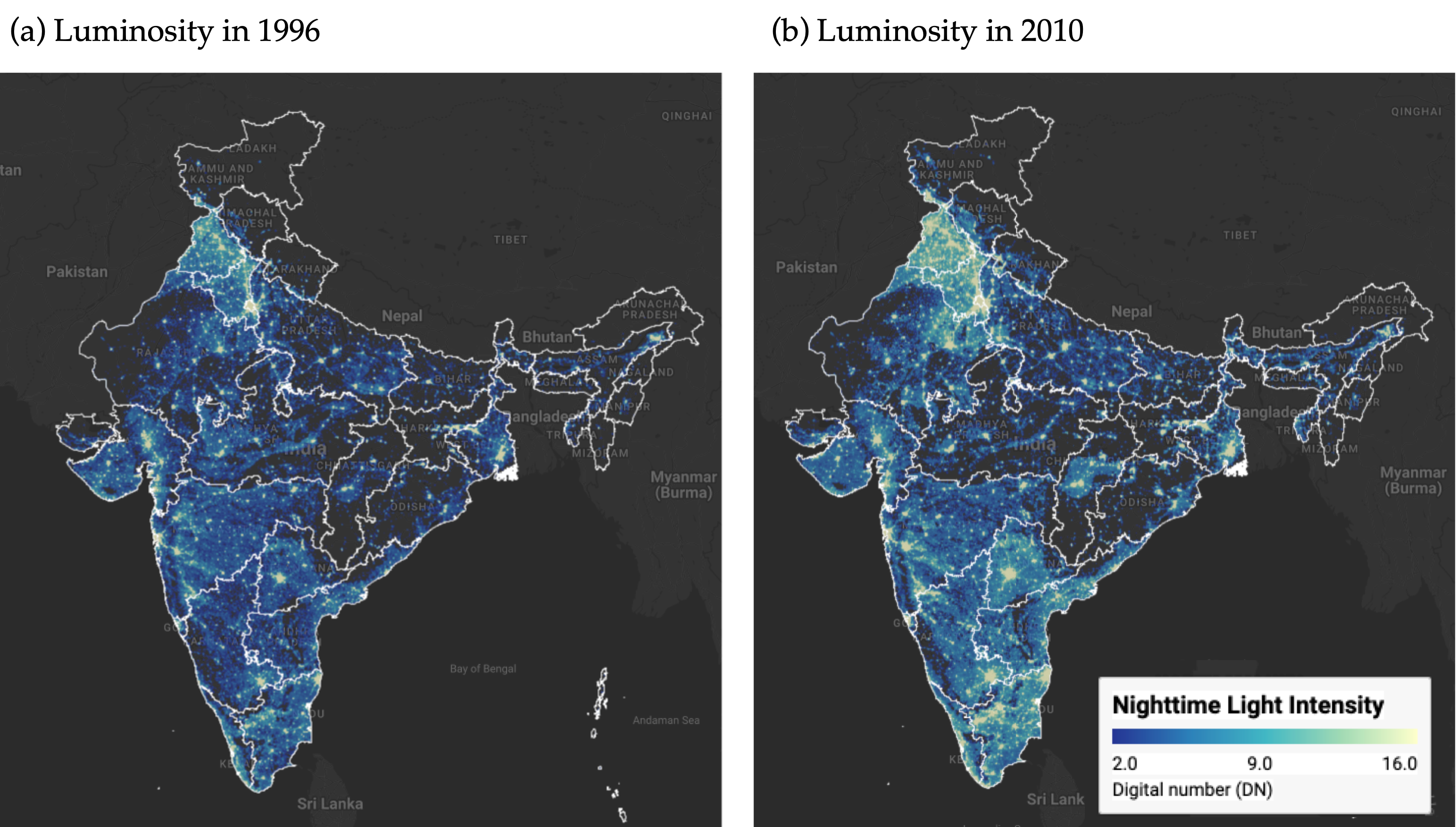
. <br> Source: Authors' visualization using pre-processed luminosity images from the Earth Observation Group (NOAA/NCEI). See [View from outer space](https://quarcs-lab.github.io/project2025s-py/notebooks/c01_view_from_space.html) notebook for source code.](images/luminosity_map.png){#fig-map}
@fig-map presents static maps (captured from our interactive application) of luminosity for the initial and final years (1996 and 2010).
The maps show a noticeable increase in brightness across most parts of India in 2010.
Since nighttime lights serve as a proxy for economic activity, this increase in luminosity reflects economic growth over the period.
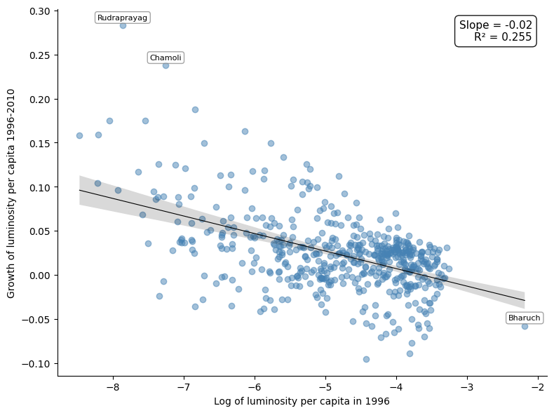
@fig-convergence illustrates the relationship between per-capita growth in nighttime lights and initial per-capita nighttime light.
The scatterplot shows an inverse relationship: the estimated $\beta$-convergence coefficient of about $-0.02$ implies an annual speed of convergence of roughly 2.3% and a half-life of about 30 years, consistent with the seminal finding of @barro_sala_convergence.
{{< embed notebooks/c02_regional_convergence_sc.ipynb#fig-convergence >}}
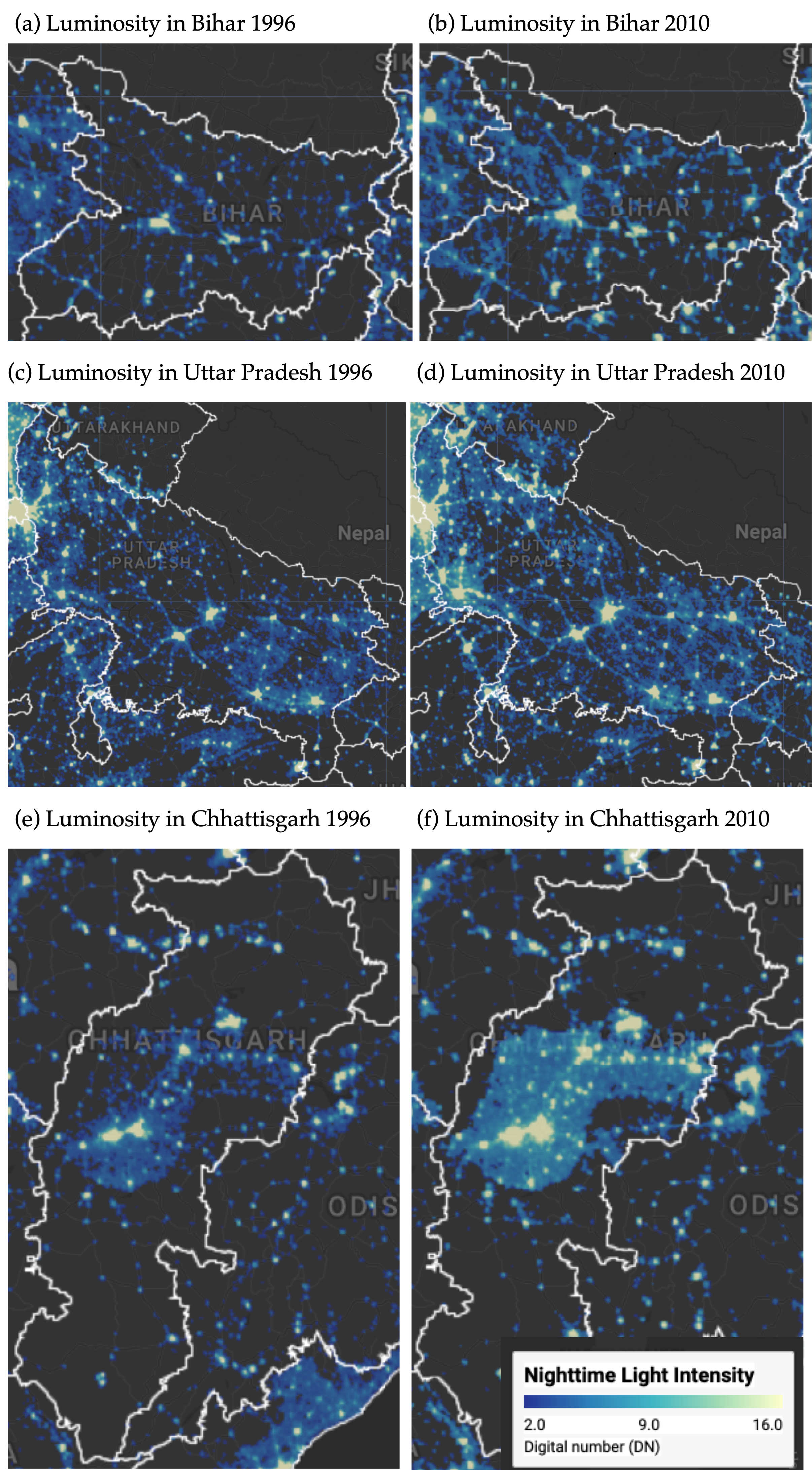
Next, we examine case studies of three economically disadvantaged states in India to illustrate their growth patterns over the study period.
Among these, Bihar is the poorest, with a per-capita income at 39.2% of the national average, while Uttar Pradesh and Chhattisgarh have per-capita incomes of 43.8% and 52.3% of the national average, respectively.[^3]
@fig-map2 displays the change in luminosity in these three states during our study period.
Although these states remain among the poorest, there is a noticeable increase in luminosity over the course of the study.
[^3]: The data are taken from a report by the Economic Advisory Council to the Prime Minister (EAC-PM), released on September 18, 2024.
. <br> Source: Authors' visualization using pre-processed luminosity images from the Earth Observation Group (NOAA/NCEI). See [View from outer space](https://quarcs-lab.github.io/project2025s-py/notebooks/c01_view_from_space.html) notebook for source code.](images/luminosity_map2.png){#fig-map2 width=75%}
### Spatial dependence is a feature of the convergence process
Before proceeding with formal econometric analysis, we examine the spatial distribution of the variables under study.
Choropleth maps provide a natural tool for this purpose, as they allow researchers to visualize how a variable of interest varies across geographic units.
They also help identify spatial patterns that may not be apparent from summary statistics alone.
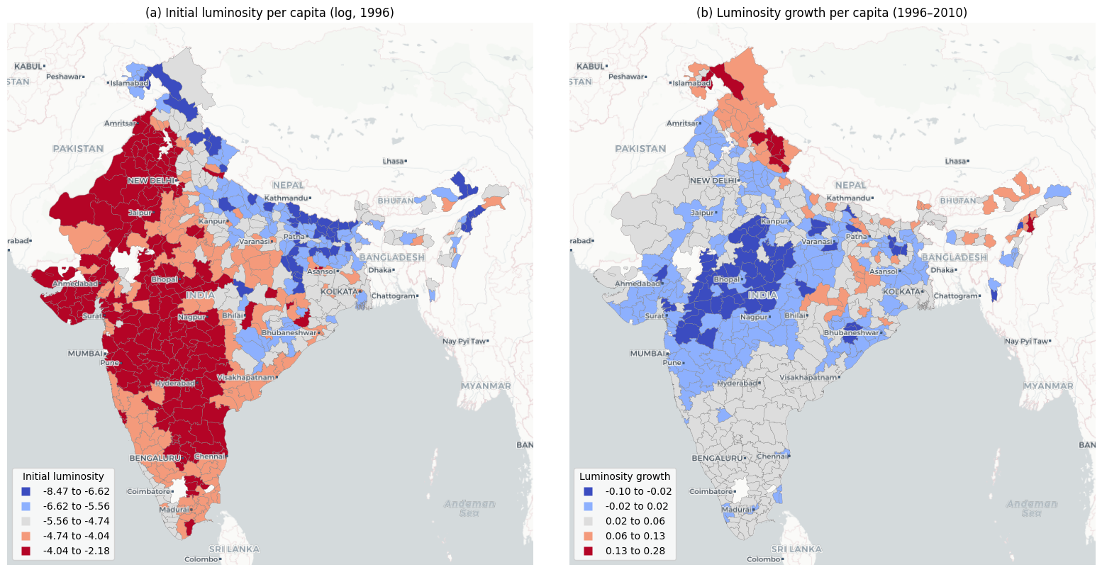
@fig-chorophleths presents the spatial distribution of initial luminosity in 1996 and the subsequent growth rate of luminosity over the 1996--2010 period across the 520 districts in our sample.
{{< embed notebooks/c03_spatial_dependence_lisa.ipynb#fig-chorophleths >}}
The choropleth maps in @fig-chorophleths reveal a distinct spatial pattern.
Panel (a) shows that initial luminosity levels are concentrated in specific geographic corridors, with higher values clustered along western coastal areas while large portions of central and eastern India exhibit markedly lower luminosity.
Panel (b), which displays the growth rate of luminosity per capita over the study period, presents a pattern that is largely the inverse of the initial distribution.
Districts that were initially bright tend to exhibit lower growth rates, whereas districts that were initially dim tend to grow at a faster rate.
This spatial inversion provides a first visual indication that regional convergence in India may have an important spatial dimension.
While the choropleth maps visually suggest the presence of spatial structures in both variables, a formal analysis of spatial dependence requires the definition of a neighborhood for each district.
This neighborhood structure is specified through a spatial weight matrix, which encodes the connectivity between geographic units.
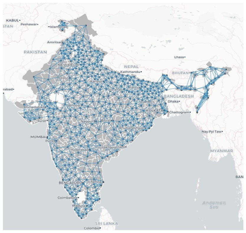
In this study, we adopt a six nearest neighbors weight matrix, whereby for each of the 520 districts, the six geographically closest districts are identified as its neighbors.
This connectivity structure is visualized as a network in @fig-wmatrix6nn, where each node represents a district centroid and each edge connects a district to one of its six nearest neighbors.
{{< embed notebooks/c03_spatial_dependence_lisa.ipynb#fig-Wmatrix6nn >}}
With the neighborhood of each district defined, we can formally assess the degree of spatial dependence in the variables.
The notion of spatial dependence can be understood through two complementary concepts.
The first is the overall degree of spatial clustering in the data, and the second is the specific locations of statistically significant clusters and spatial outliers.
The Global Moran's I statistic captures the first of these concepts.
It typically ranges from $-1$ (indicating perfect spatial dispersion) to $+1$ (indicating perfect spatial clustering), with values near zero suggesting spatial randomness.
In the context of our data, the Moran's I for initial luminosity per capita is 0.73 ($p = 0.001$), indicating a strong degree of positive spatial autocorrelation.
Districts with high (low) initial luminosity tend to be surrounded by districts that also exhibit high (low) initial luminosity.
Similarly, the Moran's I for luminosity growth is 0.60 ($p = 0.001$), confirming that the growth rates of neighboring districts are also significantly correlated.
Together, these statistics provide further evidence that both the initial level and subsequent growth of luminosity exhibit substantial spatial clustering.
While the Global Moran's I confirms the overall presence of spatial dependence, it does not reveal the location of statistically significant clusters and outliers.
To address this limitation, we employ Local Indicators of Spatial Association (LISA).
These indicators decompose the global statistic into district-level contributions and classify each district into one of four categories.
High-High (HH) indicates a district with a high value surrounded by neighbors with similarly high values, while Low-Low (LL) indicates a low-value district surrounded by low-value neighbors.
High-Low (HL) is a spatial outlier where a high-value district is surrounded by low-value neighbors, and Low-High (LH) is the opposite spatial outlier.
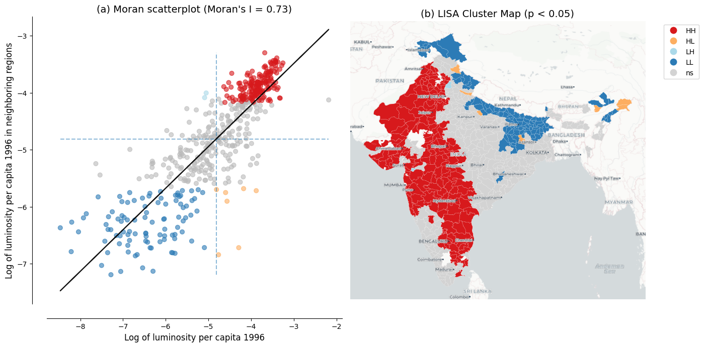
@fig-dependence-initial presents the Moran scatterplot and LISA cluster map for initial luminosity per capita.
The cluster map identifies distinct geographic concentrations: HH clusters mark the most luminous regions and their bright neighbors, while LL clusters highlight contiguous areas of low luminosity, predominantly in central and eastern India.
{{< embed notebooks/c03_spatial_dependence_lisa.ipynb#fig-dependence-initial >}}
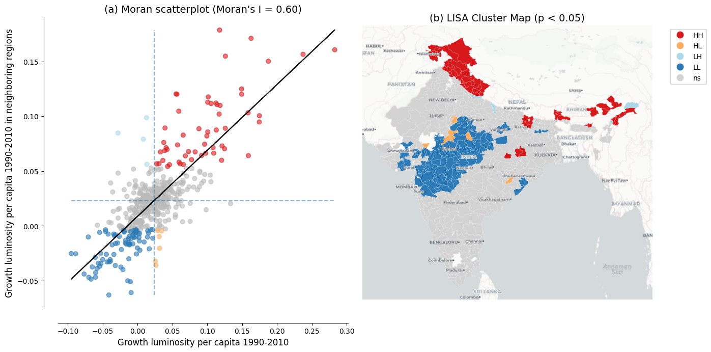
The same LISA analysis applied to luminosity growth rates reveals a geographic pattern that is largely the inverse of the initial luminosity clusters, as shown in @fig-dependence-growth.
Regions that were classified as HH clusters in initial luminosity---the brightest districts and their neighbors---tend to appear as LL clusters in luminosity growth.
This indicates that these initially prosperous areas experienced relatively slower growth over the study period.
Conversely, districts that formed LL clusters in initial luminosity---the dimmest regions---tend to emerge as HH clusters in growth, reflecting faster catch-up growth in initially lagging areas.
This spatial inversion between the initial level and subsequent growth of luminosity is the spatial signature of the convergence process: red regions in the initial luminosity map become blue regions in the growth map, and vice versa.
These local spatial patterns provide visual evidence that spatial dependence is a prominent feature of the regional convergence process observed in India.
This finding motivates the use of spatial econometric methods to formally account for these strong spatial interdependencies.
{{< embed notebooks/c03_spatial_dependence_lisa.ipynb#fig-dependence-growth >}}
### Evidence of spatial spillovers in regional convergence
The regression results of @tbl-models provide evidence of both unconditional and conditional convergence across districts in India.
Both conventional ordinary least squares (OLS) and spatial econometric approaches indicate significant negative relationships between initial luminosity levels and subsequent growth rates.
The direct effects, representing within-district convergence, remain stable across specifications, ranging from -0.020 to -0.026.
This consistency across different model specifications and estimation methods suggests that poorer districts are catching up to their wealthier counterparts, even after controlling for various district characteristics and state-level fixed effects.
{{< embed notebooks/c04_spillover_modeling_6nn.ipynb#tbl-models >}}
The progression from unconditional to conditional specifications reveals how the estimated convergence process is shaped by the inclusion of additional covariates.
In the OLS specifications, the direct effect strengthens from -0.020 to -0.022 in the unconditional models (Models 1 and 2) to -0.025 once district characteristics are added (Models 3 and 4), showing that omitting these characteristics attenuates the estimated speed of convergence.
The spatial Durbin direct effects match this pattern in the conditional models (-0.026 in Model 3 and -0.025 in Model 4).
In the unconditional models, however, the impact decomposition is unreliable: the spatial autoregressive parameter is very large (around 0.8 in Model 1), which inflates the Model 1 direct effect to -0.026.
Once we account for structural differences across districts---such as population density, urbanization, or sectoral composition---the underlying tendency for poorer districts to catch up becomes more pronounced.
The inclusion of state fixed effects, which capture unobserved state-level heterogeneity such as differences in governance and institutional quality, further sharpens the estimates by absorbing variation that might otherwise confound the convergence relationship.
The spatial Durbin model also reveals spatial spillover effects that are not captured by traditional OLS estimations.
These indirect effects, which capture the influence of neighboring districts' initial conditions on a district's growth rate, follow a notable pattern across specifications.
In the unconditional models (Models 1 and 2), the estimated indirect effects are statistically insignificant and erratic---negative in Model 2 but positive in Model 1---reflecting how, without controls, the strong residual spatial dependence confounds the spillover estimates with omitted variables.
However, once district-level controls are introduced (Models 3 and 4), the indirect effects become both larger in magnitude and statistically significant at the 10% level, reaching -0.015 in Model 3 and -0.013 in our most comprehensive Model 4.
This emergence of significant spillover effects in the conditional specifications indicates that the spatial channels of convergence become discernible only after accounting for district-specific characteristics.
The total impact of initial conditions on growth, combining both direct and spillover effects, is substantially larger when we account for spatial dependence.
In our fully specified model (Model 4), the total convergence effect in the spatial Durbin model (-0.037) is approximately 48% larger in magnitude than the OLS estimate (-0.025).
Translated into an annual speed of convergence, this raises the implied speed from about 3.0% under OLS to about 5.2% under the SDM, shortening the implied half-life from roughly 23 to 13 years.
The gap is even larger in Model 3 (SDM total -0.041 vs. OLS -0.025, or 64%), but because the Model 3 and Model 4 spillover estimates are statistically indistinguishable we anchor our interpretation on the preferred Model 4.
These differences indicate that conventional non-spatial approaches may underestimate the speed of regional convergence by failing to capture the additional convergence channels created through spatial spillovers.
The model fit statistics further support the spatial econometric approach.
The Akaike Information Criterion (AIC) consistently favors the spatial Durbin model over OLS across all four specifications.
The most comprehensive model (Model 4 SDM) achieves the lowest AIC value of -2501 compared to -2465 for the corresponding OLS.
Notably, the improvement from incorporating spatial structure is most pronounced in the unconditional specification (Model 1).
The AIC drops by 347 units when moving from OLS to SDM, reflecting the large amount of spatial dependence left unmodeled by ordinary regressions.
Even in the fully specified model, where state fixed effects already absorb much of the spatial heterogeneity, the SDM retains a meaningful advantage.
Overall, these results suggest that regional convergence in India operates not only through district-specific factors but also through spatial interactions between neighboring districts.
Ignoring these interactions leads to both underestimated convergence speeds and inferior model performance.
### Robustness to alternative spatial weight matrices
The spillover results above use a six-nearest-neighbor (6NN) spatial weight matrix.
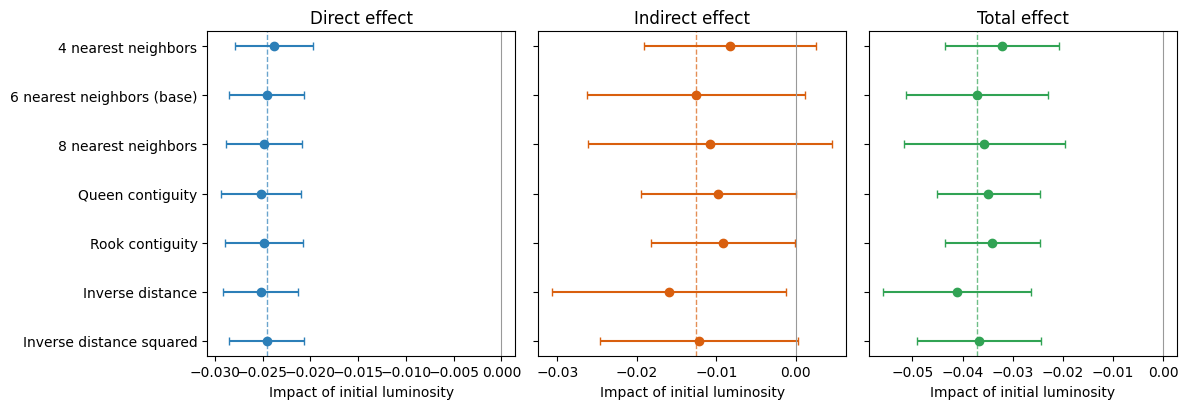
To assess their sensitivity to this choice, we re-estimate the preferred Model 4 under six alternative specifications---four- and eight-nearest neighbors, queen and rook contiguity, and inverse distance and inverse-distance-squared (each applied within a distance band)---and compare them with the 6NN baseline.
{{< embed notebooks/c07_alternative_w_matrices.ipynb#fig-altw >}}
{{< embed notebooks/c07_alternative_w_matrices.ipynb#tbl-altw >}}
The convergence spillovers are robust to the choice of spatial weights (@fig-altw and @tbl-altw).
The direct (within-district) convergence effect is essentially unchanged across all seven specifications, ranging from -0.024 to -0.026 and always significant at the 1% level.
The total convergence effect likewise remains negative and significant throughout, ranging from -0.032 to -0.041, with the 6NN baseline (-0.037) near the middle of this range.
The indirect (spillover) component is negative in every specification and statistically significant under most of them.
This stability indicates that the evidence for spatial spillovers in the convergence process is not an artifact of the particular neighbor definition, but a consistent feature of the data.
## Discussion
### Beyond the economy: Luminosity and cultural factors
Nighttime lights capture not just GDP but a composite of electrification, urbanization, infrastructure, and broader socioeconomic conditions [@henderson_storeygard_weil_lights; @mellander_etal_lights_gdp].
This multi-dimensional nature invites exploration of how luminosity relates to socioeconomic indicators beyond strictly economic output.
In this section, we examine the association between luminosity and cultural participation patterns across Indian states.
A growing literature argues that regional cultural attitudes constitute an independent factor in economic development, not merely a by-product of income or institutions.
In particular, @tubadji_cultural_entropy proposes a Culture-Based Development framework arguing that regional cultural participation patterns---measured through revealed preferences in household expenditure and survey data---predict regional development patterns.
For India, the National Sample Survey (NSS) 47th Round (July--December 1991) provides state-level data on six dimensions of cultural participation: live cultural performance, cultural telecast (TV/media), socio-cultural participation, cultural heritage and religion, live cultural shows, and sports.
With nighttime lights data for an adjacent period (1992) now available for 32 Indian states and union territories, we can examine the extent to which luminosity is associated with regional cultural patterns (see [Spatial culture](https://quarcs-lab.github.io/project2025s-py/notebooks/c06_spatial_culture.html) notebook for details and extended analyses).
Given the small sample size (N = 32) and the potential leverage of small territories at the extremes of the distribution on linear correlation measures, we report Spearman rank correlations throughout this section.
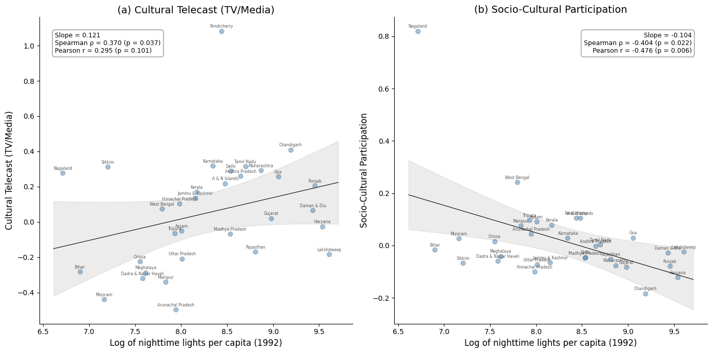
@fig-culture-scatter presents the relationship between log nighttime lights per capita and the two cultural dimensions that show statistically significant associations.
{{< embed notebooks/c06_spatial_culture.ipynb#fig-culture-scatter >}}
Cultural telecast (TV/media) exhibits a positive association (Spearman $\rho$ = 0.370, $p$ = 0.037) with nighttime light luminosity.
That is, states with higher luminosity consume more culture through television and media.
This link is intuitive: access to television depends on electrification and urbanization, which are closely tied to luminosity.
In contrast, socio-cultural participation shows a significant negative association (Spearman $\rho$ = $-$0.404, $p$ = 0.022).
That is, community-based cultural engagement is stronger in states with less luminosity.
This suggests that less urbanized regions rely more on collective, in-person forms of cultural participation rather than on media infrastructure.
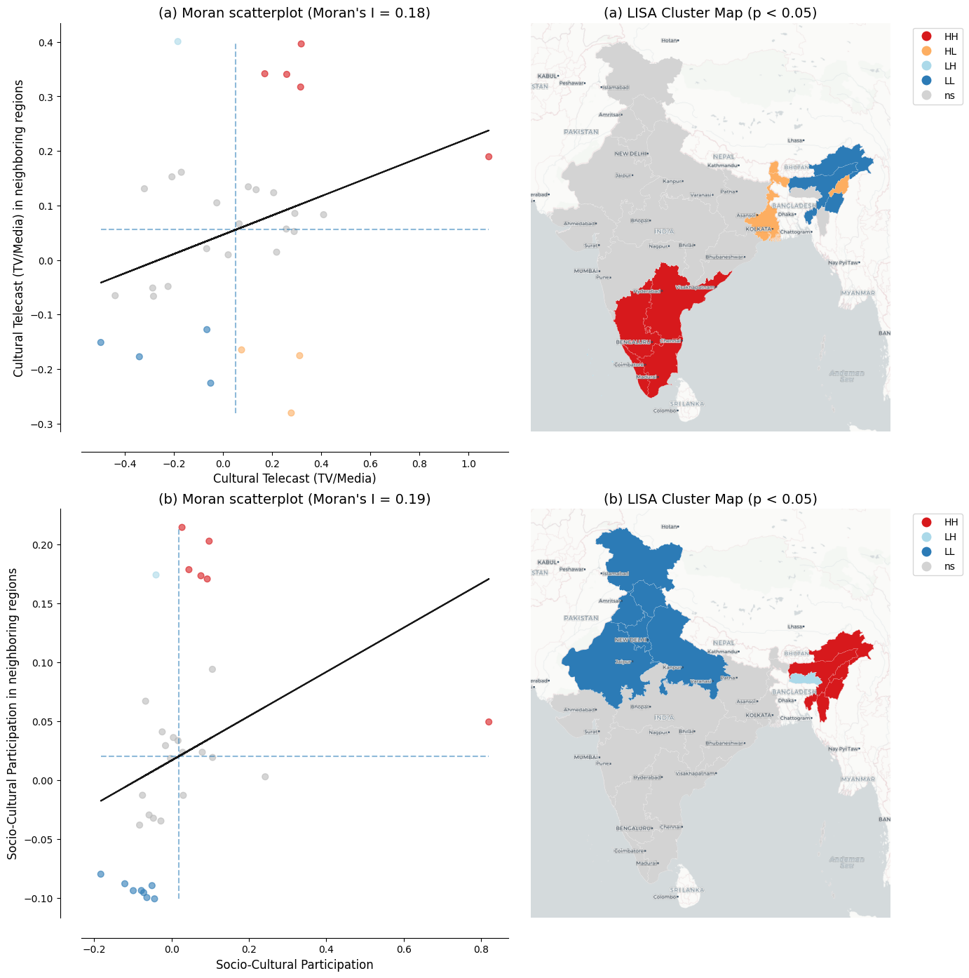
@fig-culture-lisa presents spatial distribution of these two cultural variables through the lens of a LISA analysis.
Both dimensions exhibit significant spatial autocorrelation, indicating that cultural participation is not randomly distributed across Indian states.
The spatial clustering of cultural telecast broadly mirrors the economic geography distribution.
States in the western and southern regions form high-high clusters while northeastern and eastern states form distinct community-participation clusters.
{{< embed notebooks/c06_spatial_culture.ipynb#fig-culture-lisa >}}
Together, these two results reveal a contrast in how regions engage with culture: more luminous states favor media-based consumption, while less luminous states sustain community-based participation.
The remaining four cultural dimensions---live cultural performance, cultural heritage and religion, live cultural shows, and sports---show no statistically significant association with luminosity.
However, these findings are based on a small cross-section of 32 states observed at a single point in time.
Further investigation with larger datasets covering more regions and additional time periods is needed to establish whether these patterns are robust.
### Better luminosity data from VIIRS
Our analysis, following @chanda_kabiraj_district_convergence, relies on radiance-calibrated DMSP-OLS nighttime lights data covering the period 1996 to 2010.
This dataset has been widely used as a proxy for economic activity [@henderson_storeygard_weil_lights; @chen_nordhaus_luminosity_gdp].
However, DMSP-OLS data are subject to well-documented limitations, including top-coding in bright urban cores and lack of on-board calibration leading to inter-satellite inconsistencies.
Blooming artifacts that spatially blur light sources beyond their true boundaries represent an additional concern [@abrahams_etal_deblurring].
These measurement issues can attenuate the precision of convergence estimates, particularly in rapidly urbanizing districts.
The Visible Infrared Imaging Radiometer Suite (VIIRS), operational since 2012, represents a marked improvement over DMSP-OLS along multiple dimensions.
VIIRS offers finer spatial resolution (approximately 750 meters versus 2.7 kilometers) and on-board radiometric calibration that provides consistent quantitative measurements.
It also features a wider dynamic range that avoids saturation in urban areas while detecting dim lights in rural settlements [@elvidge_etal_viirs].
Systematic assessments recommend VIIRS as the preferred product for cross-sectional and recent time-series studies [@gibson_etal_ntl_measurement].
Future extensions of our convergence analysis using VIIRS data could yield more precise estimates of both direct and indirect effects, especially in districts where blooming effects may have distorted the true spillover effects.
A practical challenge for extending long-run convergence studies is the discontinuity between DMSP (1992--2013) and VIIRS (2012--present) sensor eras.
Recent harmonization efforts, notably the global harmonized nighttime light dataset by @li_etal_harmonization, have created consistent long-run time series by calibrating VIIRS observations to DMSP-equivalent units during the overlap period.
Such harmonized datasets could enable the extension of our spatial Durbin analysis to more recent periods.
This would allow researchers to examine whether the convergence patterns and spatial spillovers documented here have persisted, accelerated, or changed in character as India's economy has continued to transform.
### New research directions
While our analysis documents the average convergence effect and its spatial spillover component, the cross-sectional regression framework does not capture potential heterogeneity in convergence patterns across the income distribution.
Distribution dynamics approaches, as pioneered by @quah_twin_peaks, could reveal whether Indian districts are converging to a single steady state or forming distinct convergence clubs where districts converge within groups but diverge across them.
The regression tree methods developed by @durlauf_johnson_convergence_clubs for identifying multiple growth regimes could be combined with spatial econometric techniques.
Such an approach could examine whether geographic clusters of districts follow distinct convergence trajectories, potentially revealing spatial poverty traps or growth poles that are not visible in average convergence estimates [@rey_spatial_dynamics].
Furthermore, analysis of harmonized luminosity data across Chinese provinces has uncovered complex inequality dynamics that differ markedly across cross-sectional and temporal dimensions [@glawe_mendez_china_luminosity].
Extending these insights to the Indian district context could help determine whether the convergence patterns we document reflect a single equilibrium or mask the formation of distinct spatial clubs.
Another important direction concerns the causal identification of the spillover channels that our spatial Durbin model captures in reduced form.
While our estimates document significant indirect effects, the model does not identify whether these spillovers operate through infrastructure linkages, labor migration, technology diffusion, or market access channels.
Quasi-experimental approaches, such as those employed by @asher_novosad_rural_roads to study the causal effects of rural road construction on structural transformation in India, could be embedded within spatial econometric frameworks to isolate specific spillover mechanisms.
Understanding which channels drive the indirect convergence effects is important for designing spatially targeted policies that may amplify positive spillovers.
Comparative evidence from other developing economies suggests that spatial dependence in regional convergence is a widespread phenomenon rather than an India-specific feature.
Studies have documented significant spatial spillover effects in convergence processes across Thailand [@tipayalai_mendez_thailand], Turkey [@ursavas_mendez_turkey], and Indonesian districts [@miranti_mendez_indonesia], with neighbor effects and spatial conditioning factors playing important roles in shaping convergence trajectories.
This cross-country regularity strengthens the case for systematic investigation of the specific mechanisms driving spatial spillovers, as the channels may differ across institutional and geographic contexts.
The growing availability of diverse satellite products and machine learning methods opens possibilities for richer measurement of regional economic activity.
@jean_etal_poverty_prediction showed that combining high-resolution daytime imagery with nighttime lights through deep learning can considerably improve poverty prediction in data-scarce settings.
Similarly, @keola_etal_lights_poverty showed that integrating nighttime lights with land cover data improves economic measurement in agricultural areas where lights alone provide weak signals.
These alternative data sources allow the construction of multi-dimensional proxies for regional economic activity that go beyond what nighttime lights alone can capture.
Recent applications demonstrate the practical potential of these advances for subnational economic measurement.
@chen_etal_turkey_viirs show that higher-quality VIIRS nighttime lights can predict sectoral GDP composition across Turkish provinces, distinguishing between urban service-oriented and rural agricultural regions in ways that DMSP data cannot.
@hussein_etal_vietnam_ml employ machine learning methods with multiple remote sensing indicators to predict subnational GDP in Vietnam, achieving accuracy improvements over traditional luminosity-based approaches.
At a broader scale, @theara_etal_cambodia_poverty combine big data sources, socioeconomic surveys, and machine learning to map multidimensional poverty in Cambodia, illustrating how satellite-derived features can complement conventional survey instruments.
Applying similar multi-source approaches to Indian districts could yield richer proxies for economic activity that overcome the well-known limitations of nighttime lights in agricultural and low-density areas.
### Research reproducibility and open science
The complexity of satellite-based economic research---involving multi-step data processing pipelines, spatial econometric estimation, and geographic visualization---makes reproducibility both challenging and essential.
As @donaldson_storeygard_remotesensing note, the processing of satellite data requires careful documentation and sharing of code to ensure that results can be replicated and extended.
Each methodological choice in the pipeline, from sensor inter-calibration to spatial weight matrix construction, can affect empirical conclusions.
This underscores the need for transparent computational workflows that allow other researchers to verify and build upon published findings.
This article adopts a reproducible research approach through Jupyter notebooks and the Quarto publishing framework.
All computational analyses are documented in embedded notebooks that readers can inspect alongside the results they produce.
The interactive visualization tool, built on Google Earth Engine, allows researchers to explore the spatial and temporal patterns in satellite nighttime light data.
Open-source tools and cloud computing platforms are rapidly lowering the barriers to reproducible spatial economic research.
Cloud-based computational notebooks, such as those developed by @mendez_patnaik_notebook for processing nighttime lights data, eliminate the need for specialized local software and provide accessible workflows for data ingestion, preprocessing, spatial analysis, and visualization.
The combination of open data repositories, version-controlled code, and cloud computing infrastructure creates an ecosystem where the full analytical pipeline---from satellite imagery to econometric results---can be made transparent, verifiable, and extensible by the broader research community.
## Concluding remarks
This article re-examines the regional convergence hypothesis across Indian districts using satellite nighttime light data, interactive visualizations, and spatial econometric modeling.
Building on the work of @chanda_kabiraj_district_convergence, we developed an interactive web-based visualization tool that illustrates spatial and convergence patterns across Indian districts.
Spatial autocorrelation analyses indicate that spatial dependence is a notable characteristic of satellite data and the regional convergence process in India.
Estimates from our spatial Durbin model indicate that incorporating spatial spillovers increases the estimated speed of regional convergence.
The total convergence effect in our fully specified model is approximately 48% larger than conventional non-spatial estimates.
This finding suggests that non-spatial convergence models may underestimate the speed of regional convergence.
Additionally, it suggests that place-based development interventions may have broader impacts, as their benefits can extend to neighboring districts through spatial spillover effects.
Our results also demonstrate the usefulness of satellite nighttime lights for studying economic dynamics in countries where subnational data are scarce, infrequent, or unreliable.
Conventional economic statistics at the district level are often unavailable or inconsistent across administrative boundaries, especially in large developing economies.
Radiance-calibrated nighttime light data allowed us to analyze 520 Indian districts at a spatial granularity that would be difficult to achieve with traditional national accounts.
This data-driven approach is potentially transferable to other data-poor contexts across the developing world.
The ongoing transition from DMSP-OLS to the higher-resolution VIIRS sensor should yield more precise measurement of subnational economic activity in future studies.
This study also shows how reproducible open-science practices can strengthen the credibility and reach of scientific research.
The entire analytical pipeline is documented in computational Jupyter notebooks using Python, R, and Stata code.
Research results are automatically embedded within the manuscript through Quarto's publishing framework.
Moreover, a single manuscript source generates multiple output formats: HTML, PDF, Microsoft Word, among others.
The HTML version is particularly useful as it allows readers to engage with interactive visualizations, easily inspect the code of multiple computational notebooks, and reevaluate the results in light of their source code.
By hosting the complete codebase and data in a public GitHub repository and making the Python notebooks executable in the cloud through Google Colaboratory, we aim to encourage broader adoption of reproducible open-science practices.
## Acknowledgments {.appendix}
This research project was supported by JSPS KAKENHI Grant Number 24K04884.
During the preparation of this manuscript, the authors acknowledge the use of Claude Code (Anthropic) to assist with manuscript editing, computational notebook development, and research infrastructure setup.
After using this AI tool, the authors reviewed the outputs, confirmed their accuracy, and take full responsibility for the content of this publication.
## Conflict of Interest {.appendix}
The authors declare no conflict of interest.
## Data and Code Availability {.appendix}
All data and computational code used in this study are available in the project repository: [Repository URL removed for blind review].
The interactive HTML version of this manuscript (<https://quarcs-lab.github.io/project2025s-py/>) embeds the computational notebooks, allowing readers to inspect the complete analytical pipeline from raw data to published results.
All notebooks can be executed in the cloud using Google Colaboratory without requiring local software installation.
The computational notebooks are implemented entirely in Python; an earlier implementation of the same analysis used R and Stata, and the present Python results are largely consistent with it---the only material difference being the impact decomposition of the unconditional spatial Durbin model (Model 1), whose total effect is unchanged.