2 Growth theory preliminaries
2.1 Why do we care about growth?
It is hard to put it better than Nobel laureate Robert Lucas did as he mused on the importance of the study of economic growth for macroeconomists and for anyone interested in economic development.1
’The diversity across countries in measured per capita income levels is literally too great to be believed. (…) Rates of growth of real per capita GNP are also diverse, even over sustained periods. For 1960-80 we observe, for example: India, 1.4% per year; Egypt, 3.4%; South Korea, 7.0%; Japan, 7.1%; the United States, 2.3%; the industrial economies averaged 3.6%. (..) An Indian will, on average, be twice as well off as his grandfather; a Korean 32 times. (…) I do not see how one can look at figures like these without seeing them as representing possibilities. Is there some action a government of India could take that would lead the Indian economy to grow like Indonesia’s or Egypt’s? If so, what, exactly? If not, what is it about the ’nature of India’ that makes it so? The consequences for human welfare involved in questions like these are simply staggering: Once one starts to think about them, it is hard to think about anything else.’
Lucas Jr. (1988) (emphasis added)
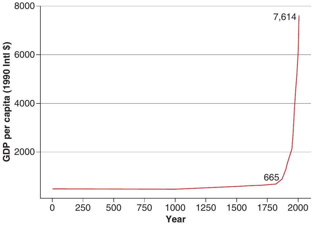
While it is common to think about growth today as being somehow natural, even expected - in fact, if world growth falls from 3.5 to \(3.2 \%\), it is perceived as a big crisis - it is worthwhile to acknowledge that this was not always the case. Pretty much until the end of the 18th century growth was quite low, if it happened at all. In fact, it was so low that people could not see it during their lifetimes. They lived in the same world as their parents and grandparents. For many years it seemed that growth was actually behind as people contemplated the feats of antiquity without understanding how they could have been accomplished. Then, towards the turn of the 18th century, as shown in Figure 2.1, something happened that created explosive economic growth as the world had never seen before. Understanding this transition will be the purpose of Chapter 10. Since then, growth has become the norm. This is the reason the first half of this book, in fact up to Chapter 10, will deal with understanding growth. As we proceed we will ask about the determinants of capital accumulation (Chapters 2 through 5, as well as 8 and 9), and discuss the process of technological progress (Chapter 6). Institutional factors will be addressed in Chapter 7. The growth process raises many interesting questions: should we expect this growth to continue? Should we expect it eventually to decelerate? Or, on the contrary, will it accelerate without bound?
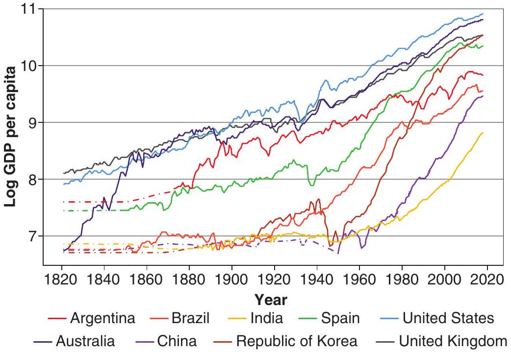
But the fundamental point of Lucas’s quote is to realise that the mind-boggling differences in income per capita across countries are to a large extent due to differences in growth rates over time; and the power of exponential growth means that even relatively small differences in the latter will build into huge differences in the former. Figures 2.2 and 2.3 make this point. The richest countries have been growing steadily over the last two centuries, and some countries have managed to converge to their income levels. Some of the performances are really stellar. Figure 2.2 shows how South Korea, with an income level that was \(16 \%\) of that of the U.S. in 1940, managed to catch up in just a few decades. Today its income is \(68.5 \%\) compared to the U.S. Likewise, Spain’s income in 1950 was \(23 \%\) that of the U.S. Today it is 57%. At the same time other countries lagged. Argentina for example dropped from an income level that was \(57 \%\) of U.S. income at the turn of the century to \(33.5 \%\) today.
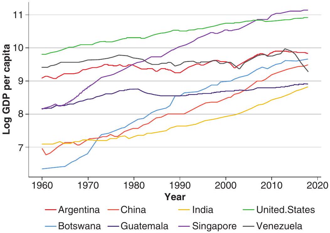
Figure 2.3 shows some diversity during recent times. The spectacular performances of Botswana, Singapore or, more recently, of China and India, contrast with the stagnation of Guatemala, Argentina or Venezuela. In 1960 the income of the average Motswana (as someone from Botswana is called) was only \(6 \%\) as rich as the average Venezuelan. In 2018 he or she was \(48 \%\) richer!
These are crucial reasons why we will spend about the initial half of this book in understanding growth. But those are not the only reasons! You may be aware that macroeconomists disagree on a lot of things; however, the issue of economic growth is one where there is much more of a consensus. It is thus helpful to start off on this relatively more solid footing. Even more importantly, the study of economic growth brings to the forefront two key ingredients of essentially all of macroeconomic analysis: general equilibrium and dynamics. First, understanding the behaviour of an entire economy requires thinking about how different markets interact and affect one another, which inevitably requires a general equilibrium approach. Second, to think seriously about how an economy evolves over time we must consider how today’s choices affect tomorrow’s - in other words, we must think dynamically! As such, economic growth is the perfect background upon which to develop the main methodological tools in macroeconomics: the model of intertemporal optimisation, known as the neoclassical growth model (NGM for short, also known as the Ramsey model), and the overlapping generations model (we’ll call it the OLG model). A lot of what we will do later, as we explore different macroeconomic policy issues, will involve applications of these dynamic general-equilibrium tools that we will learn in the context of studying economic growth.
So, without further delay, to this we turn.
2.2 The Kaldor facts
What are the key stylised facts about growth that our models should try to match? That there is growth in output and capital per worker with relatively stable income shares.
The modern study of economic growth starts in the post-war period and was mostly motivated by the experience of the developed world. In his classical article (Kaldor 1957), Nicolas Kaldor stated some basic facts that he observed economic growth seemed to satisfy, at least in those countries. These came to be known as the Kaldor facts, and the main challenge of growth theory as initially constituted was to account simultaneously for all these facts. But, what were these Kaldor facts? Here they are:2
Output per worker shows continuous growth, with no tendency to fall.
The capital/output ratio is nearly constant. (But what is capital?)
Capital per worker shows continuous growth (… follows from the other two).
The rate of return on capital is nearly constant (real interest rates are flat).
Labour and capital receive constant shares of total income.
The growth rate of output per worker differs substantially across countries (and over time, we can add, miracles and disasters).
Most of these facts have aged well. But not all of them. For example, we now know the constancy of the interest rate is not so when seen from a big historical sweep. In fact, interest rates have been on a secular downward trend that can be dated back to the 1300s (Schmelzing 2019). (Of course rates are way down now, so the question is how much lower can they go?) We will show you the data in a few pages.
In addition, in recent years, particularly since the early 1980s, the labour share has fallen significantly in most countries and industries. There is much argument in the literature as to the reasons why (see Karabarbounis and Neiman (2014) for a discussion on this) and the whole debate about income distribution trends recently spearheaded by Piketty (2014) has to do with this issue. We will come back to it shortly.
As it turns out Robert Solow established a simple model (Solow 1956) that became the first working model of economic growth.3 Solow’s contribution became the foundation of the NGM, and the backbone of modern growth theory, as it seemed to fit the Kaldor facts. Any study of growth must start with this model, reviewing what it explains - and, just as crucially, what it fails to explain.4
2.3 The Solow model
We outline and solve the basic Solow model, introducing the key concepts of the neoclassical production function, the balanced growth path, transitional dynamics, dynamic inefficiency, and convergence.
Consider an economy with only two inputs: physical capital, \(K\), and labour, \(L\). The production function is
\[ Y=F(K, L, t), \tag{2.1}\]
where \(Y\) is the flow of output produced. Assume output is a homogeneous good that can be consumed, \(C\), or invested, \(I\), to create new units of physical capital.
Let \(s\) be the fraction of output that is saved - that is, the saving rate - so that \(1-s\) is the fraction of output that is consumed. Note that \(0 \leq s \leq 1\).
Assume that capital depreciates at the constant rate \(\delta>0\). The net increase in the stock of physical capital at a point in time equals gross investment less depreciation:
\[ \dot{K}=I-\delta K=s \cdot F(K, L, t)-\delta K, \tag{2.2}\]
where a dot over a variable, such as \(\dot{K}\), denotes differentiation with respect to time. Equation (2.2) determines the dynamics of \(K\) for a given technology and labour force.
Assume the population equals the labour force, \(L\). It grows at a constant, exogenous rate, \(\dot{L} / L=\) \(n \geq 0\).5 If we normalise the number of people at time 0 to 1, then
\[ L_{t}=e^{n t} . \tag{2.3}\]
where \(L_{t}\) is labour at time \(t\).
If \(L_{t}\) is given from (2.3) and technological progress is absent, then (2.2) determines the time paths of capital, \(K\), and output, \(Y\). Such behaviour depends crucially on the properties of the production function, \(F(\cdot)\). Apparently minor differences in assumptions about \(F(\cdot)\) can generate radically different theories of economic growth.
2.3.1 The (neoclassical) production function
For now, neglect technological progress. That is, assume that \(F(\cdot)\) is independent of \(t\). This assumption will be relaxed later. Then, the production function (2.1) takes the form
\[ Y=F(K, L) . \tag{2.4}\]
Assume also the following three properties are satisfied. First, for all \(K>0\) and \(L>0, F(\cdot)\) exhibits positive and diminishing marginal products with respect to each input:
\[ \begin{array}{ll} \frac{\partial F}{\partial K}>0, & \frac{\partial^{2} F}{\partial K^{2}}<0 \\ \frac{\partial F}{\partial L}>0, & \frac{\partial^{2} F}{\partial L^{2}}<0 . \end{array} \]
Second, \(F(\cdot)\) exhibits constant returns to scale:
\[ F(\lambda K, \lambda L)=\lambda \cdot F(K, L) \text { for all } \lambda>0 . \]
Third, the marginal product of capital (or labour) approaches infinity as capital (or labour) goes to 0 and approaches 0 as capital (or labour) goes to infinity:
\[ \begin{aligned} & \lim _{K \rightarrow 0} \frac{\partial F}{\partial K}=\lim _{L \rightarrow 0} \frac{\partial F}{\partial L}=\infty, \\ & \lim _{K \rightarrow \infty} \frac{\partial F}{\partial K}=\lim _{L \rightarrow \infty} \frac{\partial F}{\partial L}=0 . \end{aligned} \]
These last properties are called Inada conditions.
We will refer to production functions satisfying those three sets of conditions as neoclassical production functions.
The condition of constant returns to scale has the convenient property that output can be written as
\[ Y=F(K, L)=L \cdot F(K / L, 1)=L \cdot f(k), \tag{2.5}\]
where \(k \equiv K / L\) is the capital-labour ratio, and the function \(f(k)\) is defined to equal \(F(k, 1)\). The production function can be written as
\[ y=f(k), \tag{2.6}\]
where \(y \equiv Y / L\) is per capita output.
One simple production function that satisfies all of the above and is often thought to provide a reasonable description of actual economies is the Cobb-Douglas function,
\[ Y=A K^{\alpha} L^{1-\alpha}, \tag{2.7}\]
where \(A>0\) is the level of the technology, and \(\alpha\) is a constant with \(0<\alpha<1\). The Cobb-Douglas function can be written as
\[ y=A k^{\alpha} . \tag{2.8}\]
Note that \(f^{\prime}(k)=A \alpha k^{\alpha-1}>0, f^{\prime \prime}(k)=-A \alpha(1-\alpha) k^{\alpha-2}<0, \lim _{k \rightarrow \infty} f^{\prime}(k)=0\), and \(\lim _{k \rightarrow 0} f^{\prime}(k)=\infty\). In short, the Cobb-Douglas specification satisfies the properties of a neoclassical production function.
2.3.2 The law of motion of capital
The change in the capital stock over time is given by (2.2). If we divide both sides of this equation by \(L\), then we get
\[ \dot{K} / L=s \cdot f(k)-\delta k . \tag{2.9}\]
The right-hand side contains per capita variables only, but the left-hand side does not. We can write \(\dot{K} / L\) as a function of \(k\) by using the fact that
\[ \dot{k} \equiv \frac{d(K / L)}{d t}=\dot{K} / L-n k, \tag{2.10}\]
where \(n=\dot{L} / L\). If we substitute (2.10) into the expression for \(\dot{K} / L\) then we can rearrange terms to get
\[ \dot{k}=s \cdot f(k)-(n+\delta) \cdot k . \tag{2.11}\]
The term \(n+\delta\) on the right-hand side of (2.11) can be thought of as the effective depreciation rate for the capital/labour ratio, \(k \equiv K / L\). If the saving rate, \(s\), were 0 , then \(k\) would decline partly due to depreciation of \(K\) at the rate \(\delta\) and partly due to the growth of \(L\) at the rate \(n\).
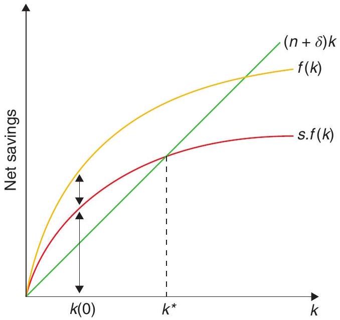
Figure 2.4 shows the workings of (2.11). The upper curve is the production function, \(f(k)\). The term \(s \cdot f(k)\) looks like the production function except for the multiplication by the positive fraction \(s\). The \(s \cdot f(k)\) curve starts from the origin (because \(f(0)=0\) ), has a positive slope (because \(f^{\prime}(k)>0\) ), and gets flatter as \(k\) rises (because \(f^{\prime \prime}(k)<0\) ). The Inada conditions imply that the \(s \cdot f(k)\) curve is vertical at \(k=0\) and becomes perfectly flat as \(k\) approaches infinity. The other term in (2.11), \((n+\delta) \cdot k\), appears in Figure 2.1 as a straight line from the origin with the positive slope \(n+\delta\).
2.3.3 Finding a balanced growth path
A balanced growth path (BGP) is a situation in which the various quantities grow at constant rates.6 In the Solow model, the BGP corresponds to \(\dot{k}=0\) in (2.11).7 We find it at the intersection of the \(s \cdot f(k)\) curve with the \((n+\delta) \cdot k\) line in Figure 2.4. The corresponding value of \(k\) is denoted \(k^{*}\). Algebraically, \(k^{*}\) satisfies the condition:
\[ s \cdot f\left(k^{*}\right)=(n+\delta) \cdot k^{*} . \tag{2.12}\]
Since \(k\) is constant in the BGP, \(y\) and \(c\) are also constant at the values \(y^{*}=f\left(k^{*}\right)\) and \(c^{*}=(1-s) \cdot f\left(k^{*}\right)\), respectively. Hence, in the Solow model, the per capita quantities \(k, y\), and \(c\) do not grow in the BGP: it is a growth model without (long-term) growth!
Now, that’s not quite right: the constancy of the per capita magnitudes means that the levels of variables - \(K, Y\), and \(C\) - grow in the BGP at the rate of population growth, \(n\). In addition, changes in the level of technology, represented by shifts of the production function, \(f(\cdot)\); in the saving rate, \(s\); in the rate of population growth, \(n\); and in the depreciation rate, \(\delta\); all have effects on the per capita levels of the various quantities in the BGP.
We can illustrate the results for the case of a Cobb-Douglas production function. The capital/ labour ratio on the BGP is determined from (2.12) as
\[ k^{*}=\left(\frac{s A}{n+\delta}\right)^{\frac{1}{1-\alpha}} . \tag{2.13}\]
Note that, as we saw graphically for a more general production function \(f(k), k^{*}\) rises with the saving rate, \(s\), and the level of technology, \(A\), and falls with the rate of population growth, \(n\), and the depreciation rate, \(\delta\). Output per capita on the BGP is given by
\[ y^{*}=A^{\frac{1}{1-\alpha}} \cdot\left(\frac{s}{n+\delta}\right)^{\frac{\alpha}{1-\alpha}} . \tag{2.14}\]
Thus, \(y^{*}\) is a positive function of \(s\) and \(A\) and a negative function of \(n\) and \(\delta\).
2.3.4 Transitional dynamics
Moreover, the Solow model does generate growth in the transition to the BGP. To see the implications in this regard, note that dividing both sides of (2.11) by \(k\) implies that the growth rate of \(k\) is given by
\[ \gamma_{k} \equiv \frac{\dot{k}}{k}=\frac{s \cdot f(k)}{k}-(n+\delta) . \tag{2.15}\]
Equation (2.15) says that \(\gamma_{k}\) equals the difference between two terms, \(s \cdot f(k) / k\) and \((n+\delta)\) which we plot against \(k\) in Figure 2.5. The first term is a downward-sloping curve, which asymptotes to infinity at \(k=0\) and approaches 0 as \(k\) tends to infinity. The second term is a horizontal line crossing the vertical axis at \(n+\delta\). The vertical distance between the curve and the line equals the growth rate of capital per person, and the crossing point corresponds to the BGP. Since \(n+\delta>0\) and \(s \cdot f(k) / k\) falls monotonically from infinity to 0 , the curve and the line intersect once and only once. Hence (except for the trivial solution \(k^{*}=0\), where capital stays at zero forever), the BGP capital-labour ratio \(k^{*}>0\) exists and is unique.
Note also that output moves according to
\[ \frac{\dot{y}}{y}=\alpha \frac{\dot{k}}{k}=\alpha \gamma_{k} . \tag{2.16}\]
A formal treatment of dynamics follows. From (2.11) one can calculate
\[ \frac{d \dot{k}}{d k}=s \cdot f^{\prime}(k)-(n+\delta) . \tag{2.17}\]
We want to study dynamics in the neighbourhood of the BGP, so we evaluate this at \(k^{*}\) :
\[ \left.\frac{d \dot{k}}{d k}\right|_{k=k^{*}}=s \cdot f^{\prime}\left(k^{*}\right)-(n+\delta) . \tag{2.18}\]
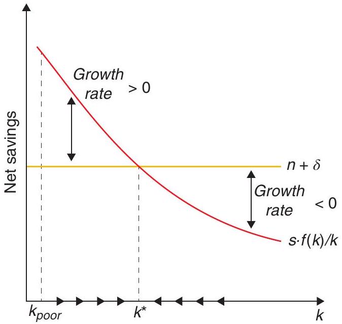
The capital stock will converge to its BGP if \(\dot{k}>0\) when \(k<k^{*}\) and \(\dot{k}<0\) when \(k>k^{*}\). Hence, this requires that \(\left.\frac{d \dot{k}}{d k}\right|_{k=k^{*}}<0\).
In the Cobb-Douglas case the condition is simple. Note that
\[ \left.\frac{d \dot{k}}{d k}\right|_{k=k^{*}}=s \cdot A \alpha\left(\frac{s A}{n+\delta}\right)^{-1}-(n+\delta)=(n+\delta)(\alpha-1) \tag{2.19}\]
so that \(\left.\frac{d \dot{k}}{d k}\right|_{k=k^{*}}<0\) requires \(\alpha<1\). That is, reaching the BGP requires diminishing returns.
With diminishing returns, when \(k\) is relatively low, the marginal product of capital, \(f^{\prime}(k)\), is relatively high. By assumption, households save and invest a constant fraction, \(s\), of this product. Hence, when \(k\) is relatively low, the marginal return to investment, \(s \cdot f^{\prime}(k)\), is relatively high. Capital per worker, \(k\), effectively depreciates at the constant rate \(n+\delta\). Consequently, the growth of capital, \(\dot{k}\), is also relatively high. In fact, for \(k<k^{*}\) it is positive. Conversely, for \(k>k^{*}\) it is negative.
2.3.5 Policy experiments
Suppose that the economy is initially on a BGP with capital per person \(k_{1}^{*}\). Imagine that the government then introduces some policy that raises the saving rate permanently from \(s_{1}\) to a higher value \(s_{2}\). Figure 2.6 shows that the \(s \cdot f(k) / k\) schedule shifts to the right. Hence, the intersection with the \(n+\delta\) line also shifts to the right, and the new BGP capital stock, \(k_{2}^{*}\), exceeds \(k_{1}^{*}\). An increase in the saving rate generates temporarily positive per capita growth rates. In the long run, the levels of \(k\) and \(y\) are permanently higher, but the per capita growth rates return to 0.
A permanent improvement in the level of the technology has similar, temporary effects on the per capita growth rates. If the production function, \(f(k)\), shifts upward in a proportional manner, then the
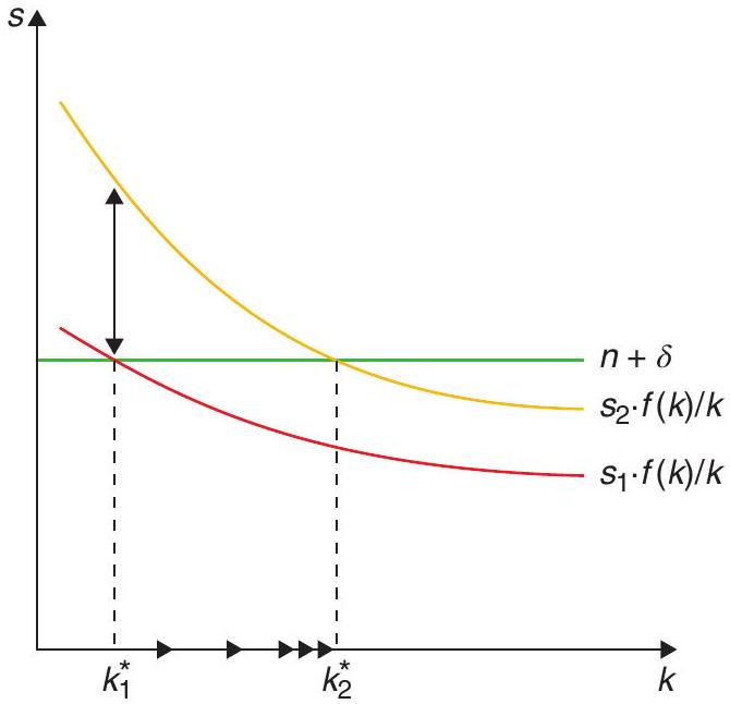
\(s \cdot f(k) / k\) curve shifts upward, just as in Figure 2.6. Hence, \(\gamma_{k}\) again becomes positive temporarily. In the long run, the permanent improvement in technology generates higher levels of \(k\) and \(y\), but no changes in the per capita growth rates.
2.3.6 Dynamic inefficiency
For a given production function and given values of \(n\) and \(\delta\), there is a unique BGP value \(k^{*}>0\) for each value of the saving rate, \(s\). Denote this relation by \(k^{*}(s)\), with \(d k^{*}(s) / d s>0\). The level of per capita consumption on the BGP is \(c^{*}=(1-s) \cdot f\left[k^{*}(s)\right]\). We know from (2.12) that \(s \cdot f\left(k^{*}\right)=(n+\delta) \cdot k^{*}\); hence we can write an expression for \(c^{*}\) as
\[ c^{*}(s)=f\left[k^{*}(s)\right]-(n+\delta) \cdot k^{*} . \tag{2.20}\]
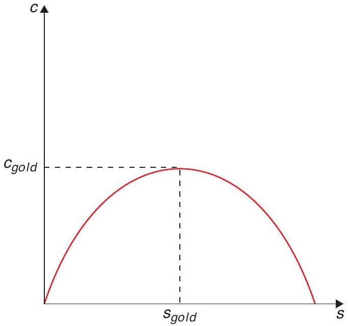
Figure 2.7 shows the relation between \(c^{*}\) and \(s\) that is implied by (2.20). The quantity \(c^{*}\) is increasing in \(s\) for low levels of \(s\) and decreasing in \(s\) for high values of \(s\). The quantity \(c^{*}\) attains its maximum when the derivative vanishes, that is, when \(\left[f^{\prime}\left(k^{*}\right)-(n+\delta)\right] \cdot d k^{*} / d s=0\). Since \(d k^{*} / d s>0\), the term in brackets must equal 0. If we denote the value of \(k^{*}\) by \(k_{g}\) that corresponds to the maximum of \(c^{*}\), then the condition that determines \(k_{g}\) is
\[ f^{\prime}\left(k_{g}\right)=(n+\delta) . \tag{2.21}\]
The corresponding savings rate can be denoted as \(s_{g}\), and the associated level of per capita consumption on the BGP is given by \(c_{g}=f\left(k_{g}\right)-(n+\delta) \cdot k_{g}\) and is is called the “golden rule” consumption rate.
If the savings rate is greater than that, then it is possible to increase consumption on the BGP, and also over the transition path. We refer to such a situation, where everyone could be made better off by an alternative allocation, as one of dynamic inefficiency. In this case, this dynamic inefficiency is brought about by oversaving: everyone could be made better off by choosing to save less and consume more. But this naturally begs the question: why would anyone pass up this opportunity? Shouldn’t we think of a better model of how people make their savings decisions? We will see about that in the next chapter.
2.3.7 Absolute and conditional convergence
Equation (2.15) implies that the derivative of \(\gamma_{k}\) with respect to \(k\) is negative:
\[ \partial \gamma_{k} / \partial k=\frac{s}{k}\left[f^{\prime}(k)-\frac{f(k)}{k}\right]<0 . \tag{2.22}\]
Other things equal, smaller values of \(k\) are associated with larger values of \(\gamma_{k}\). Does this result mean that economies with lower capital per person tend to grow faster in per capita terms? Is there convergence across economies?
We have seen above that economies that are structurally similar in the sense that they have the same values of the parameters \(s, n\), and \(\delta\) and also have the same production function, \(F(\cdot)\), have the same BGP values \(k^{*}\) and \(y^{*}\). Imagine that the only difference among the economies is the initial quantity of capital per person, \(k(0)\). The model then implies that the less-advanced economies - with lower values of \(k(0)\) and \(y(0)\) - have higher growth rates of \(k\). This hypothesis is known as conditional convergence: within a group of structurally similar economies (i.e. with similar values for \(s, n\), and \(\delta\) and production function, \(F(\cdot)\) ), poorer economies will grow faster and catch up with the richer one. This hypothesis does seem to match the data - think about how poorer European countries have grown faster, or how the U.S. South has caught up with the North, over the second half of the 20th century.
An alternative, stronger hypothesis would posit simply that poorer countries would grow faster without conditioning on any other characteristics of the economies. This is referred to as absolute convergence, and does not seem to fit the data well.8 Then again, the Solow model does not predict absolute convergence!
2.4 Can the model account for income differentials?
We have seen that the Solow model does not have growth in per capita income in the long run. But can it help us understand income differentials?
We will tackle the empirical evidence on economic growth at a much greater level of detail later on. However, right now we can ask whether the simple Solow model can account for the differences in income levels that are observed in the world. According to the World Bank’s calculations, the range of 2020 PPP income levels vary from $ 138,000 per capita in Qatar or $80,000 in Norway, all the way down to \(\$ 700\) in Burundi. Can the basic Solow model explain this difference in income per capita of a factor of more than 100 times or even close to 200 times?
In order to tackle this question we start by remembering what output is supposed to be on the BGP:
\[ y^{*}=A^{\frac{1}{1-\alpha}}\left(\frac{s}{n+\delta}\right)^{\frac{\alpha}{1-\alpha}} . \tag{2.23}\]
Assuming \(A=1\) and \(n=0\) this simplifies to:
\[ y^{*}=\left(\frac{s}{\delta}\right)^{\frac{\alpha}{1-\alpha}} . \tag{2.24}\]
The ability of the Solow model to explain these large differences in income (in the BGP), as can be seen from the expressions above, will depend critically on the value of \(\alpha\).
\[ \text { If }\left\{\begin{array}{l} \alpha=\frac{1}{3} \text { then } \frac{\alpha}{1-\alpha}=\frac{1 / 3}{2 / 3}=\frac{1}{2} \\ \alpha=\frac{1}{2} \text { then } \frac{\alpha}{1-\alpha}=\frac{1 / 2}{1 / 2}=1 \\ \alpha=\frac{2}{3} \text { then } \frac{\alpha}{1-\alpha}=\frac{2 / 3}{1 / 3}=2 \end{array}\right. \]
The standard (rough) estimate for the capital share is \(\frac{1}{3}\). Parente and Prescott (2002), however, claim that the capital share in GDP is much larger than usually accounted for because there are large intangible capital assets. In fact, they argue that the share of investment in GDP is closer to two-thirds rather than the more traditional one-third. The reasons for the unaccounted investment are (their estimates of the relevance of each in parenthesis):
Repair and maintenance (5% of GDP)
R&D (3% of GDP) multiplied by three (i.e. 9% of GDP) to take into account perfecting the manufacturing process and launching new products (the times three is not well substantiated)
Investment in software (3% of GDP)
Firms investment in organisation capital. (They think 12% is a good number.)
Learning on the job and training (10% of GDP)
Schooling (5% of GDP)
They claim all this capital has a return and that it accounts for about 56% of total GDP!
At any rate, using the equation above:
\[ \frac{y_{1}}{y_{2}}=\frac{\left(\frac{s_{1}}{\delta}\right)^{\frac{\alpha}{1-\alpha}}}{\left(\frac{s_{2}}{\delta}\right)^{\frac{\alpha}{1-\alpha}}}=\left(\frac{s_{1}}{s_{2}}\right)^{\frac{\alpha}{1-\alpha}}, \tag{2.25}\]
which we can use to estimate income level differences.
| \(\left(\frac{y_{1}}{y_{2}}-1\right) * 100\) | |||
|---|---|---|---|
| \(\frac{s_{1}}{s_{2}}\) | \(\alpha=\frac{1}{3}\) | \(\alpha=\frac{1}{2}\) | \(\alpha=\frac{2}{3}\) |
| 1 | 0% | 0% | 0% |
| 1.5 | 22% | 50% | 125% |
| 2 | 41% | 100% | 300% |
| 3 | 73% | 200% | 800% |
But even the 800% we get using the two-thirds estimate seems to be way too low relative to what we see in the data.
Alternatively, the differences in income may come from differences in total factor productivity (TFP), as captured by \(A\). The question is: how large do these differences need to be to explain the output differentials? Recall from (2.23) that
\[ y^{*}=A^{\frac{1}{1-\alpha}}\left(\frac{s}{n+\delta}\right)^{\frac{\alpha}{1-\alpha}} . \tag{2.26}\]
So if \(\alpha=2 / 3\), as suggested by Parente and Prescott (2002), then \(A^{\frac{1}{1-\alpha}}=A^{\frac{1}{1 / 3}}=A^{3}\). Now, let’s forget about \(s, \delta, n\) (for example, by assuming they are the same for all countries), and just focus on differences in \(A\). Notice that if TFP is 1/3, of the level in the other country, this indicates that the income level is then 1/27.
Parente and Prescott (2002) use this to estimate, for a group of countries, how much productivity would have to differ (relative to the United States) for us to replicate observed relative incomes over the period 1950-1988:
| Country | Relative Income | Relative TFP | |
|---|---|---|---|
| UK | 60% | → | 86% |
| Colombia | 22% | → | 64% |
| Paraguay | 16% | → | 59% |
| Pakistan | 10% | → | 51% |
These numbers appear quite plausible, so the message is that the Solow model requires substantial cross-country differences in productivity to approximate existing cross-country differences in income. This begs the question of what makes productivity so different across countries, but we will come back to this later.
2.5 The Solow model with exogenous technological change
We have seen that the Solow model does not have growth in per capita income in the long run. But that changes if we allow for technological change.
Allow now the productivity of factors to change over time. In the Cobb-Douglas case, this means that \(A\) increases over time. For simplicity, suppose that \(\dot{A} / A=a>0\). Out of the BGP, output then evolves according to
\[ \frac{\dot{y}}{y}=\frac{\dot{A}}{A}+\alpha \frac{\dot{k}}{k}=a+\alpha \gamma_{k} . \tag{2.27}\]
On the BGP, where \(k\) is constant,
\[ \frac{\dot{y}}{y}=a . \tag{2.28}\]
This is a strong prediction of the Solow model: in the long run, technological change is the only source of growth in per capita income.
Let’s now embed this improvement in technology or efficiency in workers. We can define labour input as broader than just bodies, we could call it now human capital defined by
\[ E_{t}=L_{t} \cdot e^{\lambda t}=L_{0} \cdot e^{(\lambda+n) t}, \tag{2.29}\]
where \(E\) is the amount of labor in efficiency units. The production function is
\[ Y=F\left(K_{t}, E_{t}\right) . \tag{2.30}\]
To put it in per capita efficiency terms, we define
\[ k=\frac{K}{E} . \tag{2.31}\]
So
\[ \frac{\dot{k}}{k}=\frac{\dot{K}}{K}-\frac{\dot{E}}{E}=\frac{s y}{k}-\delta-n-\lambda, \tag{2.32}\]
\[ \frac{\dot{k}}{k}=\frac{s f(k)}{k}-\delta-n-\lambda, \tag{2.33}\]
\[ \dot{k}=s f(k)-(\delta+n+\lambda) k . \tag{2.34}\]
For \(\dot{k}=0\)
\[ \frac{s f(k)}{k}=(\delta+n+\lambda) . \tag{2.35}\]
On the BGP \(\dot{k}=0\), so
\[ \frac{\dot{K}}{K}=\frac{\dot{E}}{E}=n+\lambda=\frac{\dot{Y}}{Y} . \tag{2.36}\]
But then
\[ \frac{\left(\frac{Y}{L}\right)}{\frac{Y}{L}}=\frac{\dot{Y}}{Y}-\frac{\dot{L}}{L}=\lambda \tag{2.37}\]
Notice that in this equilibrium income per person grows even on the BGP, and this accounts for all six Kaldor facts.
2.6 What have we learned?
The Solow model shows that capital accumulation by itself cannot sustain growth in per capita income in the long run. This is because accumulation runs into diminishing marginal returns. At some point the capital stock becomes large enough - and its marginal product correspondingly small enough - that a given savings rate can only provide just enough new capital to replenish ongoing depreciation and increases in labour force. Alternatively, if we introduce exogenous technological change that increases productivity, we can generate long-run growth in income per capita, but we do not really explain it. In fact, any differences in long-term growth rates come from exogenous differences in the rate of technological change - we are not explaining those differences, we are just assuming them! As a result, nothing within the model tells you what policy can do about growth in the long run.
That said, we do learn a lot about growth in the transition to the long run, about differences in income levels, and how policy can affect those things. There are clear lessons about: (i) convergence - the model predicts conditional convergence; (ii) dynamic inefficiency - it is possible to save too much in this model; and (iii) long-run differences in income - they seem to have a lot to do with differences in productivity.
Very importantly, the model also points at the directions we can take to try and understand long-term growth. We can have a better model of savings behaviour: how do we know that individuals will save what the model says they will save? And, how does that relate to the issue of dynamic inefficiency?
We can look at different assumptions about technology: maybe we can escape the shackles of diminishing returns to accumulation? Or can we think more carefully about how technological progress comes about?
These are the issues that we will address over the next few chapters.
References
Domar, E. D. (1946). Capital expansion, rate of growth, and employment. Econometrica, 137-147.
Harrod, R. F. (1939). An essay in dynamic theory. The Economic Journal, 49(193), 14-33.
Jones, C. I. & Romer, P. M. (2010). The new Kaldor facts: Ideas, institutions, population, and human capital. American Economic Journal: Macroeconomics, 2(1), 224-245.
Kaldor, N. (1957). A model of economic growth. Economic Journal, 67(268), 591-624.
Karabarbounis, L. & Neiman, B. (2014). The global decline of the labor share. The Quarterly Journal of Economics, 129(1), 61-103.
Kremer, M., Willis, J., & You, Y. (2021). Converging to convergence. NBER Macro Annual 2021. https://www.nber.org/system/files/chapters/c14560/c14560.pdf.
Lucas Jr., R. (1988). On the mechanics of economic development. Journal of Monetary Economics, 22, 3-42.
Parente, S. L. & Prescott, E. C. (2002). Barriers to riches. MIT Press.
Piketty, T. (2014). Capital in the twenty-first century. Harvard University Press.
Schmelzing, P. (2019). Eight centuries of global real rates, r-g, and the ’suprasecular’ decline, 1311-2018, Available at SSRN: https://ssrn.com/abstract=3485734 or http://dx.doi.org/10.2139/ssrn.3485734.
Solow, R. M. (1956). A contribution to the theory of economic growth. The Quarterly Journal of Economics, 70(1), 65-94.
Lucas’s words hold up very well more than three decades later, in spite of some evidently dated examples.↩︎
Once we are done with our study of economic growth, you can check the “new Kaldor facts” proposed by Jones and Romer (2010), which update the basic empirical regularities based on the progress over the subsequent half-century or so.↩︎
For those of you who are into the history of economic thought, at the time the framework to study growth was the so-called Harrod-Domar model, due to the independent contributions of (you probably guessed it…) Harrod (1939) and Domar (1946). It assumed a production function with perfect complementarity between labour and capital (“Leontieff”, as it is known to economists), and predicted that an economy would generate increasing unemployment of either labour or capital, depending on whether it saved a little or a lot. As it turns out, that was not a good description of the real world in the post-war period.↩︎
Solow eventually got a Nobel prize for his trouble, in 1987 - also for his other contributions to the study of economic growth, to which we will return. An Australian economist, Trevor Swan, also published an independently developed paper with very similar ideas at about the same time, which is why sometimes the model is referred to as the Solow-Swan model. He did not get a Nobel prize.↩︎
We will endogenise population growth in Chapter 10, when discussing unified growth theory.↩︎
The BGP is often referred to as a “steady state”, borrowing terminology from classical physics. We have noticed that talk of “steady state” tends to lead students to think of a situation where variables are not growing at all. The actual definition refers to constant growth rates, and it is only in certain cases and for certain variables, as we will see, that this constant rate happens to be zero.↩︎
You should try to show mathematically from (2.11) that, with a neoclassical production function, the only way we can have a constant growth rate \(\frac{\dot{k}}{k}\) is to have \(\dot{k}=0\).↩︎
Or does it? More recently, Kremer et al. (2021) have argued that there has been a move towards absolute convergence in the data in the 21st century… Stay tuned!↩︎