Plant the truth, watch classical SCM go wrong, watch SCSPILL recover it
The paper’s Section 5 quantifies the spillover bias with a Monte Carlo study: donor outcomes are generated from the SAR model on a rook lattice with known synthetic weights and a known spillover intensity \(\rho\), the treated unit receives effects \(\tau_t \sim \mathcal N(1, 1)\), and — the crucial part — the post-treatment donor outcomes are regenerated carrying the treated unit’s treated outcome, so the donors are contaminated exactly as the theory says. scspill.simulate reproduces that engine.
Note
This page runs 20 replications per cell at a short chain so it renders in about a minute; the paper uses 1000 replications at 6000 iterations. The benchmark case mc_grid_vs_r runs 200 replications against the frozen R results.
One replication, dissected
from scspill.simulate import scspill_sim_dgp, rook_W, make_wfrom scspill.simulate.dgp import paper_alphadgp = scspill_sim_dgp( T0=20, T1=10, N=16, W=rook_W(4, 4), # rook lattice among donors w=make_w(16), # donors 1-4 are exposed to the treated unit rho=0.3, sigma2=0.1, alpha=paper_alpha(16), # the paper's planted weights K=1, beta=[1.0], seed=1,)print(f"realized ATT: {dgp.truth.tau_post.mean():.3f}")print(f"pre-period fit is exact: max |Y0 - Yc @ alpha| = "f"{abs(dgp.Y0_pre - dgp.Yc_pre @ dgp.truth.alpha).max():.2e}")
realized ATT: 0.680
pre-period fit is exact: max |Y0 - Yc @ alpha| = 1.11e-16
run_one_sim fits three estimators on this panel — the classical simplex SCM, the Bayesian horseshoe SCM (which shares scspill’s Step 1 but ignores spillovers), and full SCSPILL — and scores each against the realized effects:
from scspill.simulate import run_one_simres = run_one_sim(dgp=dgp, m_iter=1500, burn=700, seed=1)res.metrics.round(4)
bias_ate
mse_ate
bias_point
mse_point
cover95_ate
cover95_point
method
0
0.0417
0.0017
0.0417
0.0529
NaN
NaN
SCM
1
0.0688
0.0047
0.0688
0.0085
0.0
0.0
BSCM
2
0.0032
0.0000
0.0032
0.0000
1.0
1.0
SCSPILL
A small grid
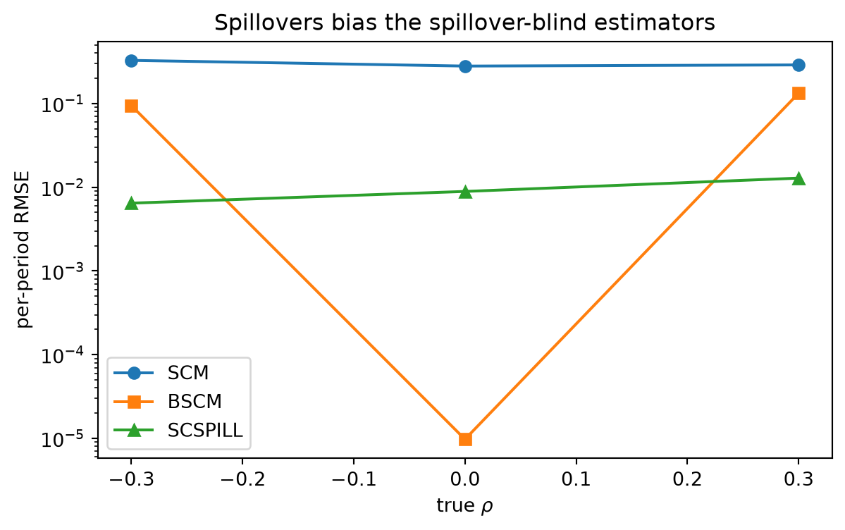
Across replications the pattern of the paper’s Tables 1–2 emerges: the classical and horseshoe-only estimators inherit a bias that grows with \(|\rho|\), while SCSPILL stays centered with near-nominal coverage.
import matplotlib.pyplot as pltfig, ax = plt.subplots(figsize=(7, 4))for method, marker in [("SCM", "o"), ("BSCM", "s"), ("SCSPILL", "^")]: sub = grid[grid["method"] == method] ax.plot(sub["rho"], sub["rmse_point"], marker=marker, label=method)ax.set_xlabel(r"true $\rho$")ax.set_ylabel("per-period RMSE")ax.set_yscale("log")ax.legend()ax.set_title("Spillovers bias the spillover-blind estimators")plt.show()
Per-period RMSE by method and true spillover intensity (20 replications per cell).
Against the frozen R results
The replication package ships the full study’s frozen output; the reduced grid tracks it closely (and the benchmark suite gates the comparison):
from pathlib import Pathfrom scspill.simulate import load_r_mc_referenceroot = Path.cwd()whilenot (root /"benchmarks").exists(): # docs pages execute in docs/articles root = root.parentref = load_r_mc_reference(root /"benchmarks"/"reference"/"mc_result")ref.query("N == 16 and T0 == 20 and rho in (-0.3, 0.0, 0.3)").round(4)
N
T0
T1
rho
method
bias_point
rmse_point
cover95_point
3
16
20
10
-0.3
SCM
-0.0633
0.3542
NaN
4
16
20
10
-0.3
BSCM
-0.0712
0.1010
0.0000
5
16
20
10
-0.3
SCSPILL
-0.0014
0.0173
0.9461
9
16
20
10
0.0
SCM
-0.0033
0.3164
NaN
10
16
20
10
0.0
BSCM
0.0000
0.0000
1.0000
11
16
20
10
0.0
SCSPILL
-0.0017
0.0257
0.9580
15
16
20
10
0.3
SCM
0.0921
0.3318
NaN
16
16
20
10
0.3
BSCM
0.1015
0.1440
0.0000
17
16
20
10
0.3
SCSPILL
-0.0030
0.0398
0.9420
At the paper’s own scale (mc_grid() with its defaults: 1000 replications, \(N \in \{16, 36, 64\}\), \(T_0 \in \{20, 50\}\), seven values of \(\rho\)) the run takes hours; pass n_jobs to parallelize across processes and backend="numba" for the JIT-compiled samplers.