The Geweke joint distribution test, prior sensitivity, and prior predictive checks
A Bayesian estimator is only as good as its sampler, so scspill ships the paper’s appendix machinery as first-class functions. This page runs each at documentation scale; the repository’s benchmark suite (benchmarks/REPORT.md) runs them long.
Note
The chains on this page are kept short so the site renders quickly; the acceptance thresholds quoted here are the ones the long-running benchmarks enforce.
The Geweke joint distribution test
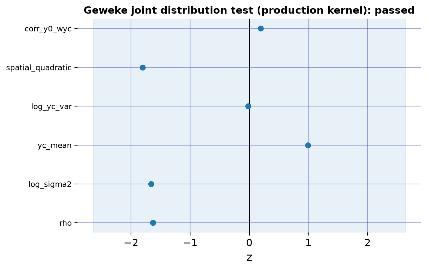
Geweke (2004) tests a posterior simulator by comparing two ways of drawing from the joint distribution \(p(\theta, y)\): exact iid draws (\(\theta \sim p(\theta)\), then \(y \mid \theta\)) against the successive-conditional chain that alternates data simulation with one full sweep of the sampler. If — and only if — every conditional is mutually consistent with the priors, the two agree in expectation for any statistic \(g(\theta, y)\).
from scspill.validation import geweke_test, plot_gewekereport = geweke_test( kernel="production", # the sampler users actually run T0=4, N=4, K=0, p=0, # a small design keeps the chain fast-mixing m_iid=8000, m_mcmc=8000, burn=1500, a0=3.0, b0=1.0, step_rho=0.5, seed=21,)report.table.round(3)
g
mean_iid
mean_mcmc
se_iid
se_mcmc
z
pval
0
rho
0.001
0.057
0.005
0.034
-1.632
0.103
1
log_sigma2
-0.914
-0.876
0.007
0.022
-1.661
0.097
2
yc_mean
-0.002
-0.009
0.005
0.005
0.993
0.321
3
log_yc_var
-0.149
-0.148
0.015
0.067
-0.020
0.984
4
spatial_quadratic
-0.974
-0.276
0.114
0.369
-1.807
0.071
5
corr_y0_wyc
-0.007
-0.009
0.006
0.008
0.192
0.848
fig = plot_geweke(report)
findfont: Failed to find font weight medium, now using 400.
findfont: Failed to find font weight medium, now using 400.
findfont: Failed to find font weight medium, now using 400.
findfont: Failed to find font weight medium, now using 400.
findfont: Failed to find font weight medium, now using 400.
findfont: Failed to find font weight medium, now using 400.
findfont: Failed to find font weight medium, now using 400.
z-scores per statistic with the Bonferroni-adjusted acceptance band.
Two practical notes, learned the hard way (details in the geweke_test docstring):
the successive-conditional chain mixes slowly when the test panel is informative — keep the design small, the Metropolis step generous, and the batch size large;
this very test caught two internal inconsistencies in the reference R implementation’s latent-factor block (see the sar model page); with the coherent parametrization every isolated sampler block passes.
Prior sensitivity
prior_sensitivity re-runs the Step-2 posterior across a grid of prior settings and support restrictions — the paper’s robustness table:
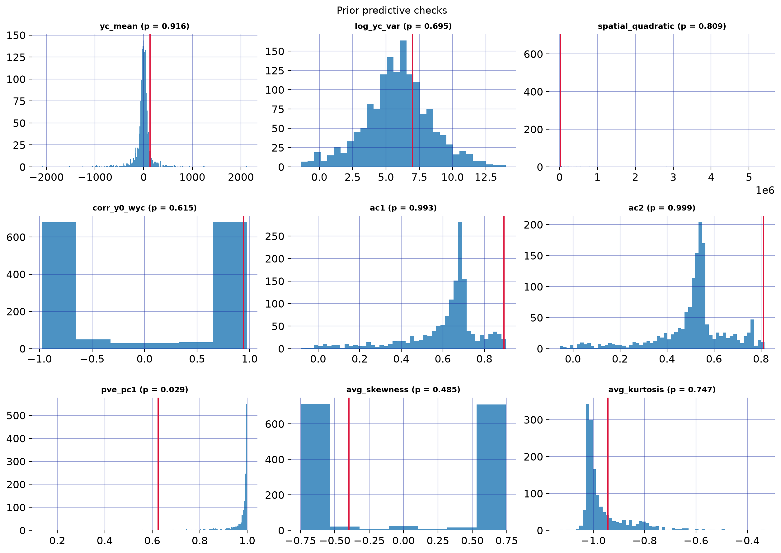
Does the model class, under its priors, generate panels that look like the observed one? prior_predictive simulates donor panels from the prior and compares nine summary statistics against the observed California panel — the p-values are \(P(h_{\text{sim}} \le h_{\text{obs}})\):
The observed statistics themselves are pinned in the test suite against the R replication package’s frozen table to three decimals — the p-values here reproduce the published pattern (the first principal component’s share of variance is the one statistic in the tail, exactly as in the paper’s appendix).
Cross-validation against the R replication package
The repository’s benchmarks/ directory runs the durable comparisons:
California and Sudan posteriors against the frozen R credible intervals (matching the R specification, and separately reporting the paper-correct one — see the sar model page for why those differ);
the reduced Monte Carlo grid against the paper’s frozen Tables 1–2 CSVs;