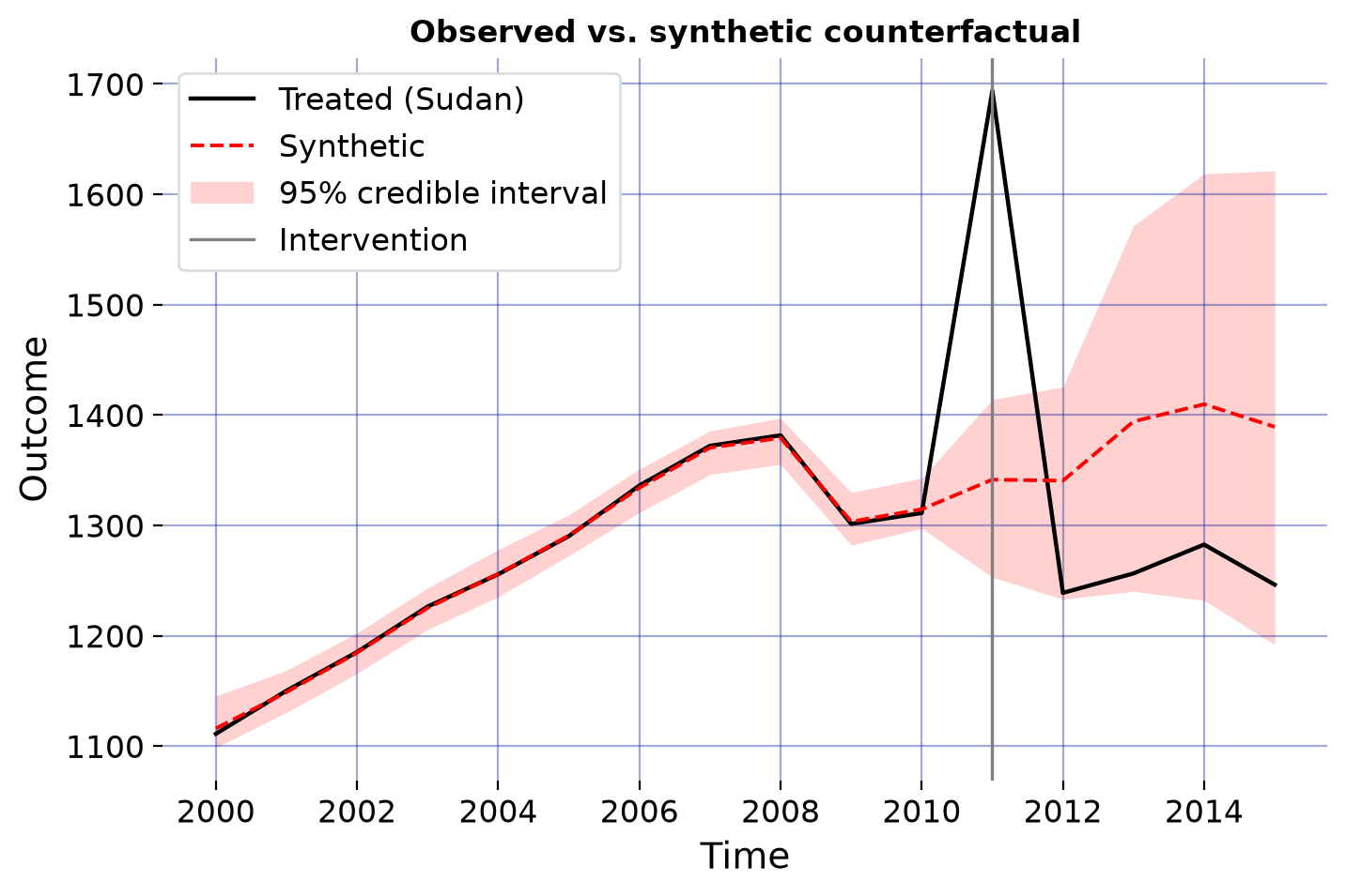
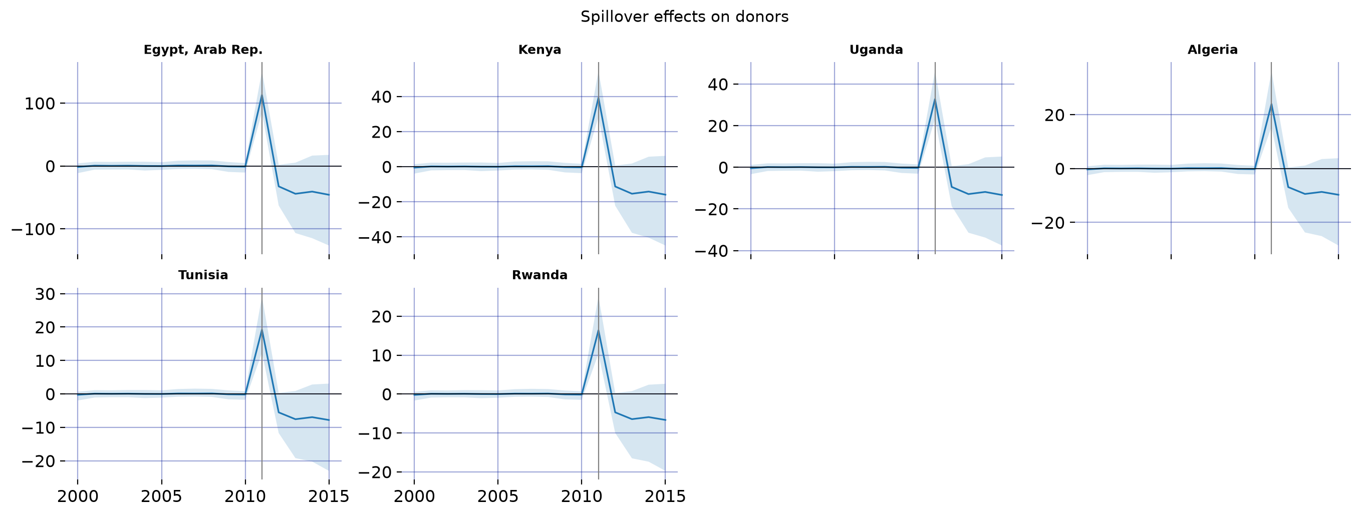
Case study: the 2011 secession of South Sudan

Spillovers along a trade network, measured in percent of GDP

In July 2011 South Sudan seceded from Sudan, taking three quarters of the oil fields with it. The paper’s second application asks what the split cost “the Sudans” (Sudan and South Sudan combined) in GDP per capita — and where the shock traveled. Spillovers here are not geographic: they move along trade links, so the spatial weights are average pre-period bilateral trade volumes rather than shared borders.

MCMC budget in this tutorial

Tutorial scale again (m_iter=4000, burn=2000). The paper’s production run for this application used one million iterations — $\rho$ mixes slowly and this panel is short ($T_0 = 11$ pre-treatment years), so treat the numbers on this page as illustrative.

Load the data

from scspill.data import load_sudan

panel = load_sudan()
panel.df.head(3)

	country_id	year	country	gdp_pc	exports_gdp_share	merchandise_trade_gdp_share	trade_gdp_share	clean_fuels_access	inflation	net_migration
0	1	2000	Algeria	3553.324205	0.420697	0.569479	0.628583	0.964	0.003392	-16454
1	1	2001	Algeria	3610.006056	0.341212	0.489334	0.545296	0.970	0.042260	-26539
2	1	2002	Algeria	3754.660815	0.331372	0.500162	0.565896	0.974	0.014183	-36255

The outcome is GDP per capita (constant 2015 US$) and six World Development Indicators enter as covariates:

panel.outcome, panel.covariates

('gdp_pc',
 ('exports_gdp_share',
  'merchandise_trade_gdp_share',
  'trade_gdp_share',
  'clean_fuels_access',
  'inflation',
  'net_migration'))

The exposure vector is raw bilateral trade with Sudan — Egypt and Kenya dominate (the estimator normalizes it internally):

panel.spatial_w.sort_values(ascending=False).head(5)

country
Egypt, Arab Rep.    3.311366e+14
Kenya               8.221436e+13
Uganda              5.884262e+13
South Africa        2.952293e+13
Tunisia             1.206114e+13
Name: amount, dtype: float64

Fit

from scspill import SCSPILL

result = SCSPILL(
    {
        **panel.config_kwargs(),
        "m_iter": 4000,
        "burn": 2000,
        "step_rho": 0.02,
        "seed": 20251022,
        "display_graphs": False,
    }
).fit()

print(f"ATT: {result.att:.1f} US$ per capita "
      f"(95% CrI [{result.att_ci[0]:.1f}, {result.att_ci[1]:.1f}])")
print(f"rho: {result.rho_hat:.3f} "
      f"(95% CrI [{result.rho_ci[0]:.3f}, {result.rho_ci[1]:.3f}])")

ATT: -31.4 US$ per capita (95% CrI [-164.7, 97.9])
rho: 0.471 (95% CrI [0.405, 0.546])

result.plot(kind="full", display=False);

findfont: Failed to find font weight medium, now using 400.
findfont: Failed to find font weight medium, now using 400.
findfont: Failed to find font weight medium, now using 400.

Observed vs. counterfactual GDP per capita for the Sudans.

Effects in percent

The paper reports the secession loss as a percentage of the counterfactual:

import numpy as np

T0 = result.inputs.T0
cf_post = result.effects_detail.cf_mean[T0:]
gap_post = result.inputs.Y0[T0:] - cf_post
years = result.inputs.time_labels[T0:]
for year, g, c in zip(years, gap_post, cf_post):
    print(f"{year}: {g:+7.1f} US$  ({100 * g / c:+5.1f}% of counterfactual)")

2011:  +352.4 US$  (+26.3% of counterfactual)
2012:  -101.7 US$  ( -7.6% of counterfactual)
2013:  -137.7 US$  ( -9.9% of counterfactual)
2014:  -127.1 US$  ( -9.0% of counterfactual)
2015:  -143.0 US$  (-10.3% of counterfactual)

Spillovers travel the trade network

result.plot(kind="spill_top", top_n=6, display=False);

findfont: Failed to find font weight medium, now using 400.

Top spillover paths: the shock lands on Sudan’s largest trade partners.

spill_post = result.spillover_panel.loc[2011:]
spill_post.abs().mean().sort_values(ascending=False).head(5).round(2)

unit
Egypt, Arab Rep.    55.30
Kenya               19.22
Uganda              16.04
Algeria             11.74
Tunisia              9.42
dtype: float64

Notes on this application

The treated unit “Sudan” aggregates Sudan and South Sudan after 2011, so the estimand is the effect of the split on the combined economy.
With $T_0 = 11$ pre-periods and 33 donors, the horseshoe prior is doing real work: it shrinks most donor weights to zero and concentrates the fit on a few economies.
$\rho$ is estimated around 0.4–0.5 here versus roughly 0.2–0.35 in the California application (depending on the specification) — trade integration transmits more of the shock than a single land border.