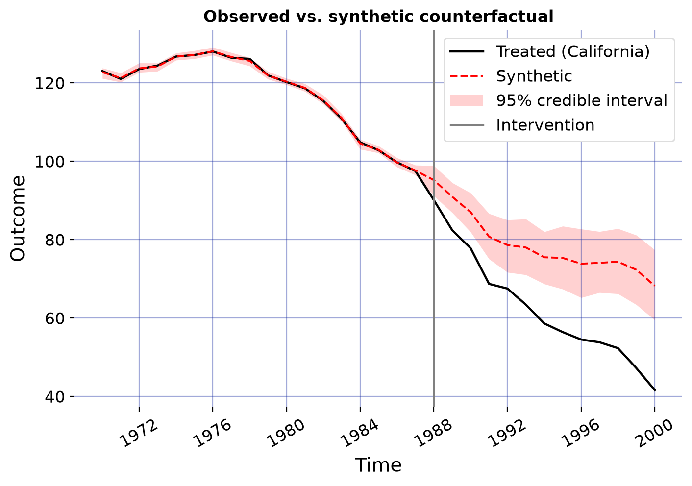
Get started: California Proposition 99

Estimate a policy effect and its spillovers with the bundled tobacco panel

In 1988 California passed Proposition 99, a large tobacco tax and control program. The classic synthetic-control analysis (Abadie, Diamond & Hainmueller 2010) builds a “synthetic California” from other states and reads the program’s effect off the gap. But cigarette taxes leak: Californians can buy cigarettes in Nevada. If the donors absorb part of the treatment, the synthetic control is contaminated and the classical estimate is biased.

scspill models that leakage explicitly. This page walks the full workflow on the bundled panel: load the data, fit the two-step Bayesian model, read the treatment effect, and — the part classical SCM cannot do — read the spillover received by each donor state.

MCMC budget in this tutorial

The pages in this documentation run a tutorial-scale chain (m_iter=4000, burn=2000, seconds on a laptop) so they render quickly. The paper’s production run for California used 100,000 iterations; for serious work use at least tens of thousands and check diagnostics().

Load the data

load_california() returns the panel plus the spatial weights, ready to splat into the estimator’s configuration:

from scspill.data import load_california

panel = load_california()
panel.df.head()

	state	state_id	year	cigsale	retprice
0	Alabama	1	1970	89.800003	39.599998
1	Alabama	1	1971	95.400002	42.700001
2	Alabama	1	1972	101.099998	42.299999
3	Alabama	1	1973	102.900002	42.099998
4	Alabama	1	1974	108.199997	43.099998

Three ingredients matter:

# 1) A 0/1 treatment column: California from 1988 onward.
panel.df.query("treated == 1").head(3)

	state	state_id	year	cigsale	retprice	treated
80	California	3	1988	90.099998	117.400002	1
81	California	3	1989	82.400002	126.400002	1
82	California	3	1990	77.800003	163.800003	1

# 2) spatial_w: how exposed is each donor to the *treated* unit?
#    Rook contiguity: Nevada is the only state in the ADH donor pool that
#    borders California (Oregon and Arizona are excluded from the pool).
panel.spatial_w[panel.spatial_w > 0]

state
Nevada    1.0
Name: adj, dtype: float64

# 3) spatial_W: donor-to-donor contiguity (row-normalized inside the estimator).
panel.spatial_W.iloc[:5, :5]

	Alabama	Arkansas	Colorado	Connecticut	Delaware
state
Alabama	0.0	0.0	0.0	0.0	0.0
Arkansas	0.0	0.0	0.0	0.0	0.0
Colorado	0.0	0.0	0.0	0.0	0.0
Connecticut	0.0	0.0	0.0	0.0	0.0
Delaware	0.0	0.0	0.0	0.0	0.0

Fit the model

from scspill import SCSPILL

result = SCSPILL(
    {
        **panel.config_kwargs(),      # df, columns, weights, covariates
        "m_iter": 4000,
        "burn": 2000,
        "seed": 20251022,
        "display_graphs": False,
    }
).fit()

Under the hood this ran the paper’s two-step sampler: a horseshoe Gibbs sampler for the synthetic weights \(\alpha\) on the 1970–1987 fit, then a spatial-autoregressive block that estimates the spillover intensity \(\rho\) (with the retail cigarette price as a covariate and one latent factor), and finally the identification formulas that turn the posterior draws into effects.

The treatment effect

print(f"ATT: {result.att:.2f} packs per capita "
      f"(95% CrI [{result.att_ci[0]:.2f}, {result.att_ci[1]:.2f}])")
print(f"rho: {result.rho_hat:.3f} "
      f"(95% CrI [{result.rho_ci[0]:.3f}, {result.rho_ci[1]:.3f}], "
      f"ESS {result.rho_ess:.0f})")

ATT: -16.13 packs per capita (95% CrI [-22.03, -10.27])
rho: 0.300 (95% CrI [0.221, 0.385], ESS 3)

result.plot(kind="full", display=False);

findfont: Failed to find font weight medium, now using 400.
findfont: Failed to find font weight medium, now using 400.
findfont: Failed to find font weight medium, now using 400.

Observed California vs. its no-treatment counterfactual, with the 95% pointwise credible band.

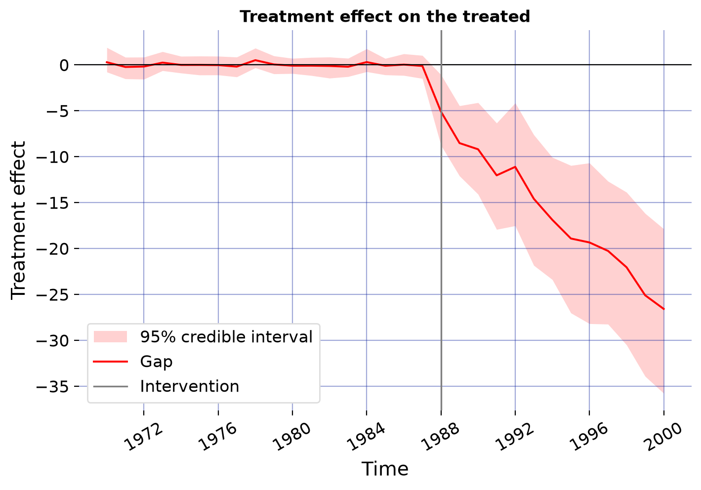
result.plot(kind="effect", display=False);

The per-year treatment effect with its credible band.

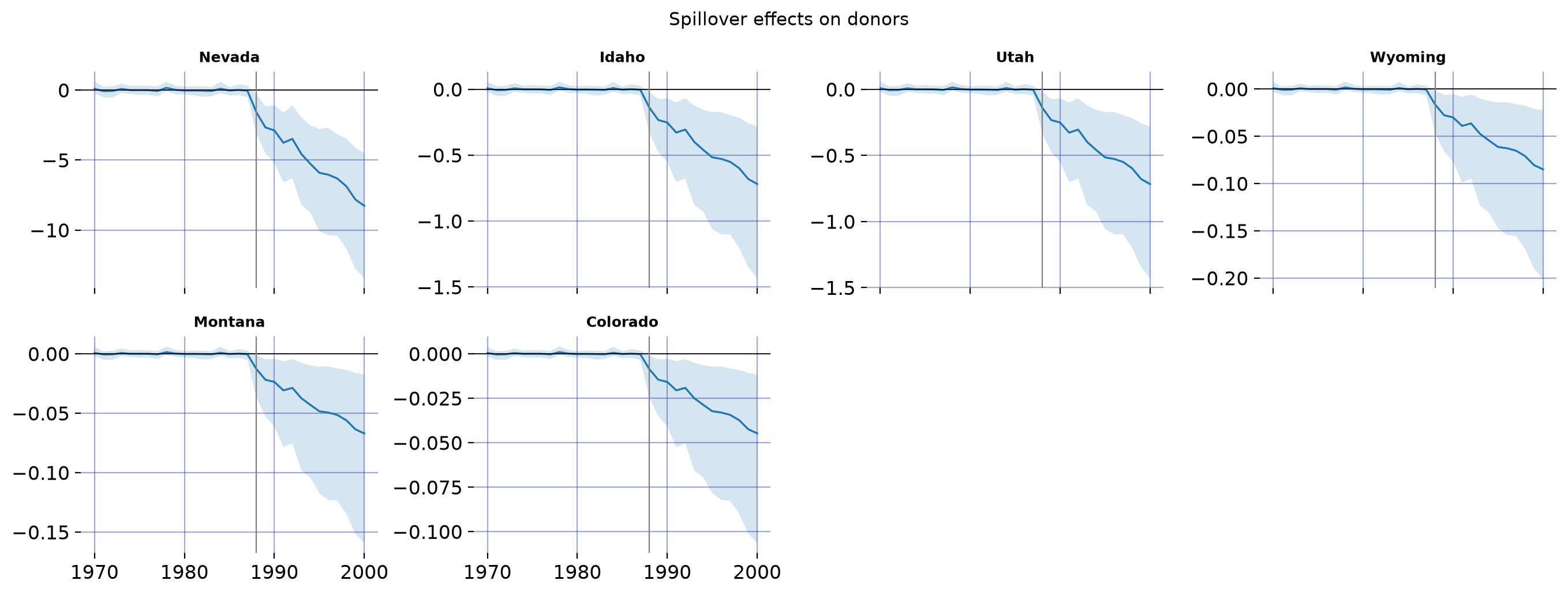
The spillovers

The identification result recovers the effect received by every donor. The spillover panel is a time-by-donor DataFrame; the plot ranks donors by their post-treatment spillover magnitude:

result.plot(kind="spill_top", top_n=6, display=False);

findfont: Failed to find font weight medium, now using 400.

Top spillover paths. Nevada — the only contiguous donor — absorbs the bulk of the leakage.

spill_post = result.spillover_panel.loc[1988:]
spill_post.abs().mean().sort_values(ascending=False).head(5).round(3)

unit
Nevada     5.034
Idaho      0.439
Utah       0.438
Wyoming    0.052
Montana    0.041
dtype: float64

Weights: horseshoe vs. the classical simplex

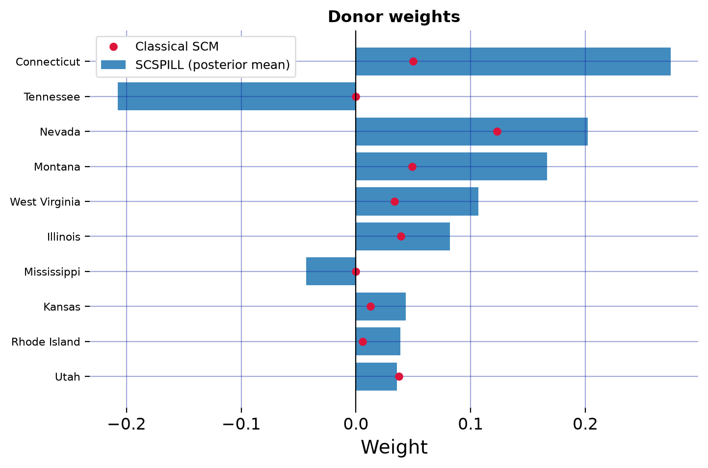
scspill’s weights are unconstrained and horseshoe-shrunk; the classical simplex weights are computed alongside for comparison:

result.plot(kind="weights", display=False);

findfont: Failed to find font weight medium, now using 400.
findfont: Failed to find font weight medium, now using 400.

Posterior-mean synthetic weights (bars) against classical simplex-SCM weights (dots).

Convergence diagnostics

result.diagnostics(top_n_alpha=4).round(3)

	mean	sd	q025	q50	q975	ess	rhat_split	mcse	geweke_z
parameter
rho	0.300	0.057	0.221	0.299	0.385	2.774	3.049	0.034	-9.861
sigma2	61.423	3.420	54.984	61.330	68.544	1685.262	1.000	0.083	0.268
alpha[Connecticut]	0.274	0.158	-0.016	0.295	0.556	102.944	1.017	0.016	1.504
alpha[Tennessee]	-0.208	0.156	-0.514	-0.215	0.015	71.322	1.000	0.018	1.117
alpha[Nevada]	0.202	0.038	0.122	0.202	0.280	238.631	1.014	0.002	-2.217
alpha[Montana]	0.167	0.137	-0.027	0.164	0.431	88.815	1.001	0.015	-0.702
beta[retprice]	0.351	0.028	0.302	0.350	0.405	5.966	1.399	0.011	3.933

\(\rho\) is the weakly identified parameter of this model — watch its ESS and run long chains for publication numbers. The validation article shows the full toolkit (Geweke test, prior sensitivity, prior predictive checks).

Where to go next

The Sudan case study: trade-network weights instead of contiguity, and spillovers measured in percent of GDP.
The sar model page: the identification result, the samplers, and exactly where this implementation deliberately departs from the R replication package.
The API reference.