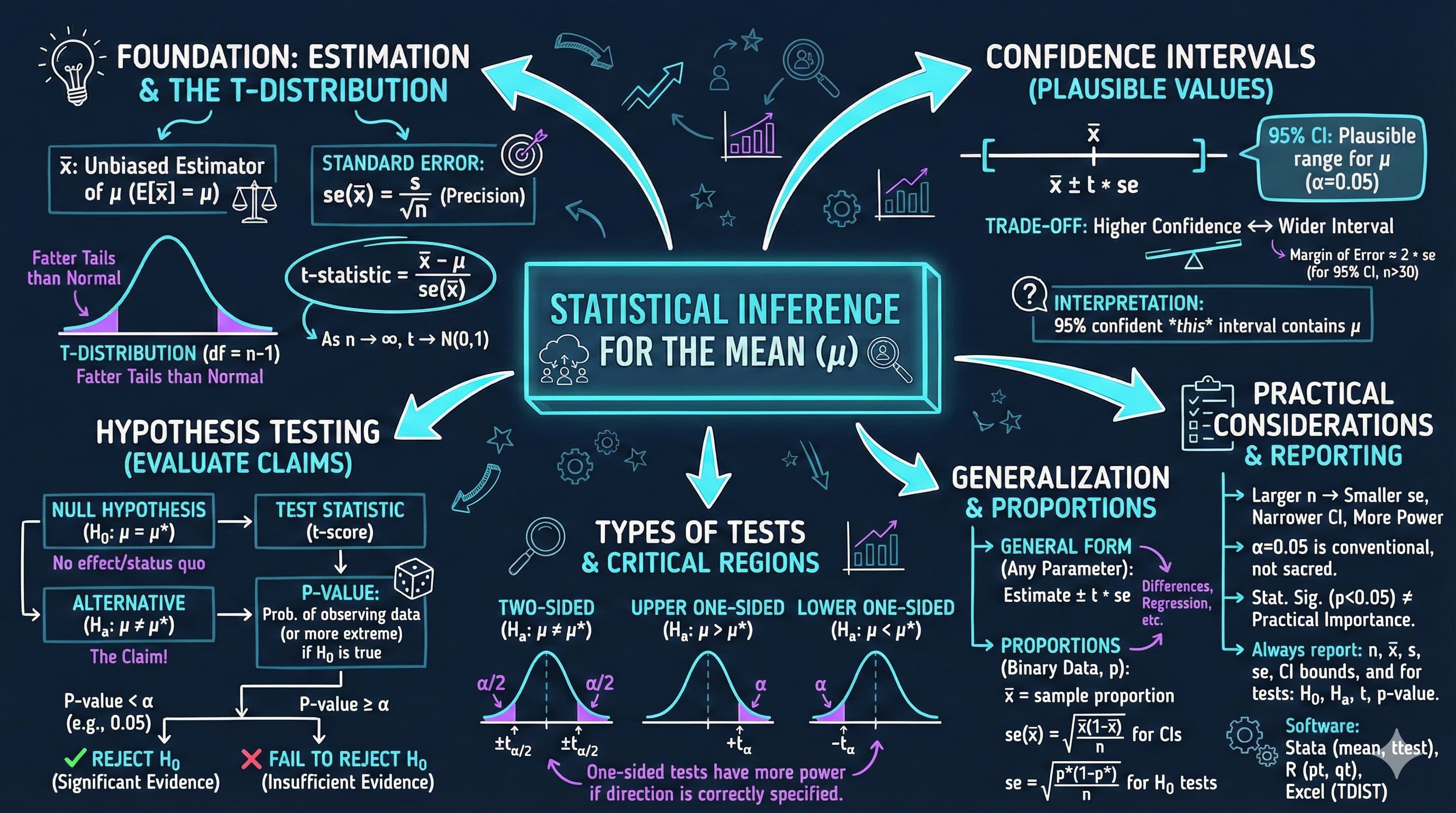
This notebook provides an interactive introduction to statistical inference, teaching you how to extrapolate from sample statistics to population parameters using confidence intervals and hypothesis tests.
This chapter introduces statistical inference for the mean—the foundational methods for extrapolating from sample statistics to population parameters with quantified uncertainty.
What you’ll learn:
Construct and interpret confidence intervals for population means
Understand the t-distribution and when to use it (vs. normal distribution)
Conduct hypothesis tests to evaluate claims about population parameters
Calculate and interpret p-values and understand statistical significance
Distinguish between one-sided and two-sided tests
Apply inference methods to proportions data and binary outcomes
Datasets used:
AED_EARNINGS.DTA: Sample of 171 30-year-old female full-time workers in 2010 (earnings in dollars)
AED_GASPRICE.DTA: Weekly gasoline prices in the U.S. (testing price level hypotheses)
AED_EARNINGSMALE.DTA: Male earnings data for hypothesis testing examples
AED_REALGDPPC.DTA: Real GDP per capita growth rates (testing economic growth hypotheses)
Chapter outline:
4.1 Example: Mean Annual Earnings
4.2 t Statistic and t Distribution
4.3 Confidence Intervals
4.4 Two-Sided Hypothesis Tests
4.5 Hypothesis Test Examples
4.6 One-Sided Directional Hypothesis Tests
4.7 Proportions Data
Setup
Run this cell first to import all required packages and configure the environment.
# Import required librariesimport numpy as npimport pandas as pdimport matplotlib.pyplot as pltimport seaborn as snsfrom scipy import statsimport randomimport os# Set random seeds for reproducibilityRANDOM_SEED =42random.seed(RANDOM_SEED)np.random.seed(RANDOM_SEED)os.environ['PYTHONHASHSEED'] =str(RANDOM_SEED)# GitHub data URL (data streams directly from here)GITHUB_DATA_URL ="https://raw.githubusercontent.com/quarcs-lab/data-open/master/AED/"# Optional: Create directories for saving outputs locallyIMAGES_DIR ='images'TABLES_DIR ='tables'os.makedirs(IMAGES_DIR, exist_ok=True)os.makedirs(TABLES_DIR, exist_ok=True)# Set plotting style (dark theme matching book design)plt.style.use('dark_background')sns.set_style("darkgrid")plt.rcParams.update({'axes.facecolor': '#1a2235','figure.facecolor': '#12162c','grid.color': '#3a4a6b','figure.figsize': (10, 6),'text.color': 'white','axes.labelcolor': 'white','xtick.color': 'white','ytick.color': 'white','axes.edgecolor': '#1a2235',})print("✓ Setup complete! All packages imported successfully.")print(f"✓ Random seed set to {RANDOM_SEED} for reproducibility.")print(f"✓ Data will stream from: {GITHUB_DATA_URL}")
✓ Setup complete! All packages imported successfully.
✓ Random seed set to 42 for reproducibility.
✓ Data will stream from: https://raw.githubusercontent.com/quarcs-lab/data-open/master/AED/
4.1 Example: Mean Annual Earnings
We’ll use a motivating example throughout this chapter: estimating the population mean annual earnings for 30-year-old female full-time workers in the U.S. in 2010.
The Problem:
We have a sample of 171 women
We want to make inferences about the population of all such women
Key Statistics:
Sample mean\(\bar{x}\): Our point estimate of population mean μ
Standard deviation s: Measures variability in the sample
Standard error se(\(\bar{x}\)) = s/√n: Measures precision of \(\bar{x}\) as an estimate of μ
The standard error is crucial—it quantifies our uncertainty about μ. Smaller standard errors mean more precise estimates.
# Load earnings datadata_earnings = pd.read_stata(GITHUB_DATA_URL +'AED_EARNINGS.DTA')earnings = data_earnings['earnings']# Calculate key statisticsn =len(earnings)mean_earnings = earnings.mean()std_earnings = earnings.std(ddof=1) # ddof=1 for sample std devse_earnings = std_earnings / np.sqrt(n) # Standard errorprint("="*70)print("SAMPLE STATISTICS FOR ANNUAL EARNINGS")print("="*70)print(f"Sample size (n): {n}")print(f"Mean: ${mean_earnings:,.2f}")print(f"Standard deviation: ${std_earnings:,.2f}")print(f"Standard error: ${se_earnings:,.2f}")print(f"\nInterpretation: Our best estimate of population mean earnings is ${mean_earnings:,.2f}")print(f"The standard error of ${se_earnings:,.2f} measures the precision of this estimate.")
======================================================================
SAMPLE STATISTICS FOR ANNUAL EARNINGS
======================================================================
Sample size (n):        171
Mean:                   $41,412.69
Standard deviation:     $25,527.05
Standard error:         $1,952.10

Interpretation: Our best estimate of population mean earnings is $41,412.69
The standard error of $1,952.10 measures the precision of this estimate.
Key Statistics from our Sample (n = 171 women):
Sample mean: $41,412.69
Standard deviation: $25,527.05
Standard error: $1,952.10
What is the standard error telling us?
The standard error of $1,952.10 measures the precision of our sample mean as an estimate of the true population mean. Think of it as quantifying our uncertainty.
Statistical interpretation:
If we repeatedly drew samples of 171 women, the sample means would vary
The standard error tells us the typical amount by which sample means differ from the true population mean
Formula: SE = s/√n = $25,527.05/√171 = $1,952.10
Why is the SE much smaller than the standard deviation?
Standard deviation ($25,527) measures variability among individual women’s earnings
Standard error ($1,952) measures variability of the sample mean across different samples
The larger the sample size, the smaller the SE → more precise estimates
Practical insight:
A standard error of $1,952 is relatively small compared to the mean ($41,413)
This suggests our estimate is reasonably precise
If we had only 43 women (n=43), SE would double to $3,904 (less precise)
With 684 women (n=684), SE would halve to $976 (more precise)
Key Concept 4.1: Standard Error and Precision
The standard error se(\(\bar{x}\)) = s/√n measures the precision of the sample mean as an estimate of the population mean μ. It quantifies sampling uncertainty—smaller standard errors mean more precise estimates. The SE decreases with sample size at rate 1/√n, so quadrupling the sample size halves the standard error.
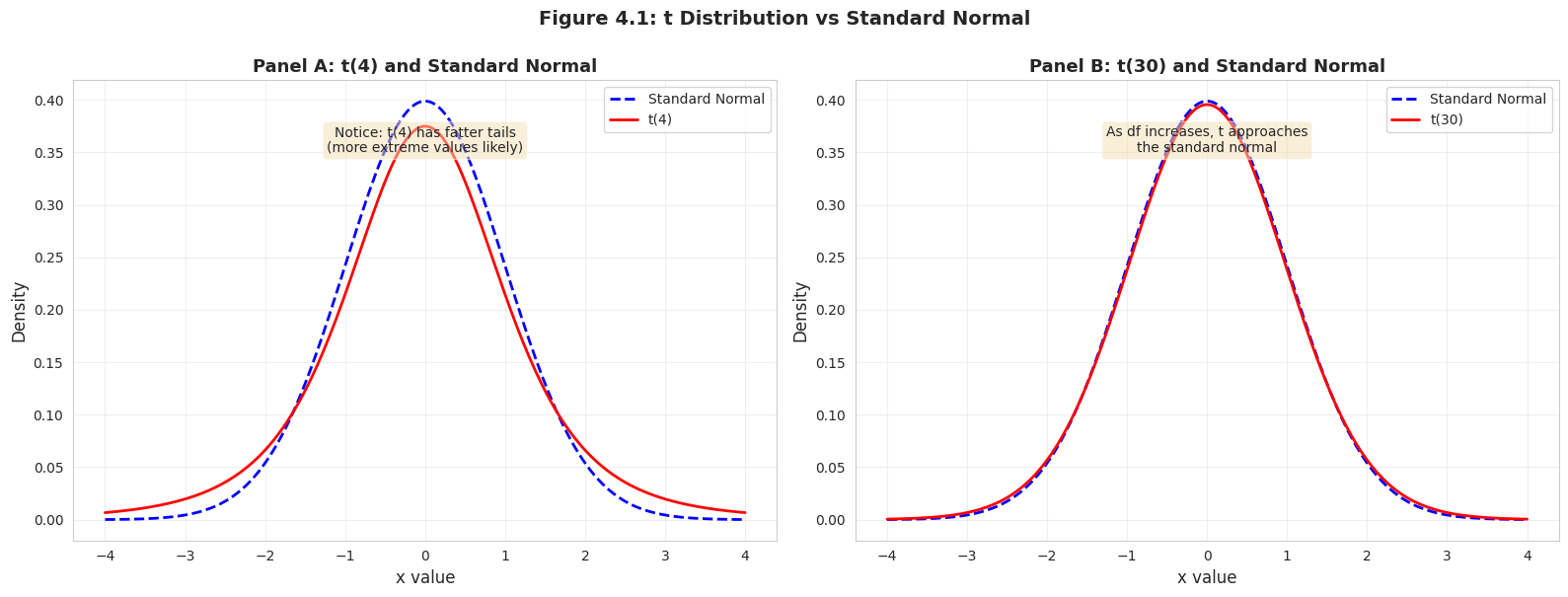
4.2 t Statistic and t Distribution
For inference on the population mean μ, we use the t-statistic:
Under certain assumptions, this statistic follows a t-distribution with (n - 1) degrees of freedom:
\[t \sim T(n-1)\]
Why t-distribution instead of normal?
We don’t know the population standard deviation σ, so we estimate it with sample std dev s
This adds uncertainty, making the distribution have fatter tails than the normal
As sample size increases (n → ∞), the t-distribution approaches the standard normal distribution
Key properties:
Symmetric around zero (like the normal)
Fatter tails than normal (more probability in extremes)
Converges to N(0,1) as degrees of freedom increase
# Visualize t-distribution vs standard normalfig, axes = plt.subplots(1, 2, figsize=(16, 6))x = np.linspace(-4, 4, 200)# Panel A: t(4) vs standard normalaxes[0].plot(x, stats.norm.pdf(x), '--', color='#c084fc', linewidth=2, label='Standard Normal')axes[0].plot(x, stats.t.pdf(x, df=4), 'r-', linewidth=2, label='t(4)')axes[0].set_xlabel('x value', fontsize=12)axes[0].set_ylabel('Density', fontsize=12)axes[0].set_title('Panel A: t(4) and Standard Normal', fontsize=13, fontweight='bold')axes[0].legend()axes[0].grid(True, alpha=0.3)axes[0].text(0, 0.35, 'Notice: t(4) has fatter tails\n(more extreme values likely)', ha='center', bbox=dict(boxstyle='round', facecolor='#1e2a45', alpha=0.9))# Panel B: t(30) vs standard normalaxes[1].plot(x, stats.norm.pdf(x), '--', color='#c084fc', linewidth=2, label='Standard Normal')axes[1].plot(x, stats.t.pdf(x, df=30), 'r-', linewidth=2, label='t(30)')axes[1].set_xlabel('x value', fontsize=12)axes[1].set_ylabel('Density', fontsize=12)axes[1].set_title('Panel B: t(30) and Standard Normal', fontsize=13, fontweight='bold')axes[1].legend()axes[1].grid(True, alpha=0.3)axes[1].text(0, 0.35, 'As df increases, t approaches\nthe standard normal', ha='center', bbox=dict(boxstyle='round', facecolor='#1e2a45', alpha=0.9))plt.suptitle('Figure 4.1: t Distribution vs Standard Normal', fontsize=14, fontweight='bold', y=1.0)plt.tight_layout()plt.show()print("\n📊 Key Observation:")print(" With more degrees of freedom (larger n), the t-distribution looks more like the normal.")print(" For n > 30, they're nearly identical.")
📊 Key Observation:
   With more degrees of freedom (larger n), the t-distribution looks more like the normal.
   For n > 30, they're nearly identical.
Key Concept 4.2: The t-Distribution
The t-distribution is used when the population standard deviation \(\sigma\) is unknown and must be estimated from the sample. It is similar to the standard normal N(0,1) but with fatter tails that reflect the additional uncertainty from estimating \(\sigma\). As the sample size \(n\) grows, the t-distribution approaches the normal distribution, making the normal a good approximation for large samples.
4.3 Confidence Intervals
A confidence interval provides a range of plausible values for the population parameter μ.
General formula:\[\text{estimate} \pm \text{critical value} \times \text{standard error}\]
For the population mean, a 100(1 - α)% confidence interval is: \[\bar{x} \pm t_{n-1, \alpha/2} \times \text{se}(\bar{x})\]
Where:
\(\bar{x}\) = sample mean (our estimate)
\(t_{n-1, \alpha/2}\) = critical value from t-distribution with (n-1) degrees of freedom
se(\(\bar{x}\)) = s/√n = standard error
α = significance level (e.g., 0.05 for 95% confidence)
Interpretation: If we repeatedly drew samples and constructed 95% CIs, about 95% of those intervals would contain the true population mean μ.
Practical interpretation: We are “95% confident” that μ lies within this interval.
Rule of thumb: For n > 30, \(t_{n-1, 0.025} \approx 2\), so a 95% CI is approximately: \[\bar{x} \pm 2 \times \text{se}(\bar{x})\]
Key Concept 4.3: Confidence Intervals
A confidence interval provides a range of plausible values for the population parameter \(\mu\). A 95% confidence interval means: if we repeated the sampling procedure many times, approximately 95% of the resulting intervals would contain the true \(\mu\). The interval is constructed as \(\bar{x} \pm t_{\alpha/2} \times se(\bar{x})\), where wider intervals indicate less precision.
# Calculate 95% confidence interval for mean earningsconf_level =0.95alpha =1- conf_levelt_crit = stats.t.ppf(1- alpha/2, n -1) # Critical valuemargin_of_error = t_crit * se_earningsci_lower = mean_earnings - margin_of_errorci_upper = mean_earnings + margin_of_errorprint("="*70)print("95% CONFIDENCE INTERVAL FOR POPULATION MEAN EARNINGS")print("="*70)print(f"Sample mean: ${mean_earnings:,.2f}")print(f"Standard error: ${se_earnings:,.2f}")print(f"Critical value t₁₇₀: {t_crit:.4f}")print(f"Margin of error: ${margin_of_error:,.2f}")print(f"\n95% Confidence Interval: [${ci_lower:,.2f}, ${ci_upper:,.2f}]")print(f"\nInterpretation: We are 95% confident that the true population mean")print(f"earnings lies between ${ci_lower:,.2f} and ${ci_upper:,.2f}.")
======================================================================
95% CONFIDENCE INTERVAL FOR POPULATION MEAN EARNINGS
======================================================================
Sample mean:            $41,412.69
Standard error:         $1,952.10
Critical value t₁₇₀:     1.9740
Margin of error:        $3,853.48

95% Confidence Interval: [$37,559.21, $45,266.17]

Interpretation: We are 95% confident that the true population mean
earnings lies between $37,559.21 and $45,266.17.
95% Confidence Interval for Mean Earnings: [$37,559.21, $45,266.17]
What this interval means:
The correct interpretation: If we repeatedly drew samples of 171 women and calculated 95% CIs for each sample, approximately 95% of those intervals would contain the true population mean μ.
Common misconceptions (WRONG interpretations):
“There is a 95% probability that μ is in this interval”
“95% of individual women earn between $37,559 and $45,266”
“The interval captures 95% of the data”
Correct interpretation:
We are 95% confident that the true population mean earnings lie between $37,559 and $45,266
The interval accounts for sampling uncertainty through the standard error
The population mean μ is fixed (but unknown); our interval is random
Breaking down the calculation:
Sample mean: $41,412.69
Critical value (t₁₇₀, 0.025): 1.9740
Margin of error: 1.9740 × $1,952.10 = $3,853.48
Interval: $41,412.69 ± $3,853.48
Practical insights:
The interval does NOT include $36,000 or $46,000, suggesting these are implausible values for μ
The interval is fairly narrow (width = $7,707), indicating good precision
The critical value (1.974) is close to 2, confirming the “rule of thumb”: CI ≈ mean ± 2×SE
Why use 95% confidence?
Convention in most scientific fields (α = 0.05)
Balances precision (narrow interval) with confidence (high probability of capturing μ)
Could use 90% (narrower, less confident) or 99% (wider, more confident)
Transition: Now that we understand how the t-distribution differs from the normal distribution, we can use it to construct confidence intervals that account for the uncertainty in estimating σ from our sample.
Confidence-Precision Trade-off
Comparing Confidence Intervals at Different Levels:
Higher confidence requires wider intervals. You cannot have both maximum precision (narrow interval) AND maximum confidence (high probability of capturing μ) simultaneously.
Why does this happen?
To be more confident we’ve captured μ, we must cast a wider net
The critical value increases with confidence level:
90% CI: t-critical ≈ 1.66 → smaller multiplier
95% CI: t-critical ≈ 1.97 → moderate multiplier
99% CI: t-critical ≈ 2.61 → larger multiplier
Practical implications:
90% CI ($6,457 width):
Narrower, more precise
BUT: 10% chance the interval misses μ
Use when: precision is critical and you can tolerate more risk
95% CI ($7,707 width):
Standard choice in economics and most sciences
Good balance between precision and confidence
Use when: following standard practice (almost always)
99% CI ($10,171 width):
Wider, less precise
BUT: Only 1% chance the interval misses μ
Use when: being wrong is very costly (medical, safety applications)
How to improve BOTH confidence AND precision?
Increase sample size (n)! Larger n → smaller SE → narrower intervals at any confidence level
With n = 684 (4× larger), the 95% CI would be approximately half as wide
Trade-off: Higher confidence → wider intervals
90% CI: Narrower, but less confident
95% CI: Standard choice (most common)
99% CI: Wider, but more confident
Let’s compare:
# Compare confidence intervals at different levelsconf_levels = [0.90, 0.95, 0.99]print("="*70)print("CONFIDENCE INTERVALS AT DIFFERENT LEVELS")print("="*70)print(f"{'Level':<10}{'Lower Bound':>15}{'Upper Bound':>15}{'Width':>15}")print("-"*70)for conf in conf_levels: alpha =1- conf t_crit = stats.t.ppf(1- alpha/2, n -1) ci_lower = mean_earnings - t_crit * se_earnings ci_upper = mean_earnings + t_crit * se_earnings width = ci_upper - ci_lowerprint(f"{conf*100:.0f}%{ci_lower:>18,.2f}{ci_upper:>18,.2f}{width:>18,.2f}")print("\n📊 Notice: Higher confidence → wider interval → less precision")
Alternative hypothesis Hₐ: What we conclude if we reject H₀ (e.g., μ ≠ $40,000)
Significance level α: Maximum probability of Type I error we’ll tolerate (typically 0.05)
Test statistic:\[t = \frac{\bar{x} - \mu_0}{\text{se}(\bar{x})}\]
Where μ₀ is the hypothesized value.
Two ways to make a decision:
p-value approach:
p-value = probability of observing a t-statistic at least as extreme as ours, assuming H₀ is true
Reject H₀ if p-value < α
Critical value approach:
Critical value c = \(t_{n-1, \alpha/2}\)
Reject H₀ if |t| > c
Both methods always give the same conclusion.
Example: Test whether population mean earnings equal $40,000.
Key Concept 4.4: Hypothesis Testing Framework
A hypothesis test evaluates whether data provide sufficient evidence to reject a specific claim (H₀) about a parameter. The t-statistic measures how many standard errors the estimate is from the hypothesized value. The p-value is the probability of observing a result at least as extreme as ours, assuming H₀ is true. Small p-values (< α, typically 0.05) provide evidence against H₀, leading us to reject it.
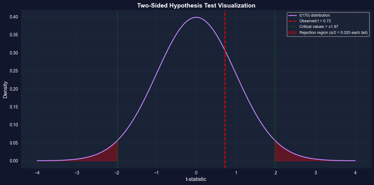
# Two-sided hypothesis test: H0: μ = $40,000 vs Ha: μ ≠ $40,000mu0 =40000# Hypothesized valuet_stat = (mean_earnings - mu0) / se_earningsp_value =2* (1- stats.t.cdf(abs(t_stat), n -1)) # Two-sided p-valuet_crit_95 = stats.t.ppf(0.975, n -1) # Critical value for α = 0.05print("="*70)print("TWO-SIDED HYPOTHESIS TEST")print("="*70)print(f"H₀: μ = ${mu0:,}")print(f"Hₐ: μ ≠ ${mu0:,}")print(f"Significance level α = 0.05")print("\nSample Statistics:")print(f" Sample mean: ${mean_earnings:,.2f}")print(f" Standard error: ${se_earnings:,.2f}")print("\nTest Results:")print(f" t-statistic: {t_stat:.4f}")print(f" p-value: {p_value:.4f}")print(f" Critical value: ±{t_crit_95:.4f}")print("\nDecision:")print(f" p-value approach: {p_value:.4f} > 0.05 → Do not reject H₀")print(f" Critical approach: |{t_stat:.4f}| < {t_crit_95:.4f} → Do not reject H₀")print("\nConclusion: We do not have sufficient evidence to reject the claim")print(f"that population mean earnings equal ${mu0:,}.")
======================================================================
TWO-SIDED HYPOTHESIS TEST
======================================================================
H₀: μ = $40,000
Hₐ: μ ≠ $40,000
Significance level α = 0.05

Sample Statistics:
  Sample mean:      $41,412.69
  Standard error:   $1,952.10

Test Results:
  t-statistic:       0.7237
  p-value:           0.4703
  Critical value:    ±1.9740

Decision:
  p-value approach:  0.4703 > 0.05 → Do not reject H₀
  Critical approach: |0.7237| < 1.9740 → Do not reject H₀

Conclusion: We do not have sufficient evidence to reject the claim
that population mean earnings equal $40,000.
Test Results: H₀: μ = $40,000 vs Hₐ: μ ≠ $40,000
t-statistic: 0.7237
p-value: 0.4703
Critical value: ±1.9740
Decision: Do NOT reject H₀
What does this mean?
We tested whether the population mean earnings equal $40,000. Based on our sample data (mean = $41,413), we do NOT have sufficient evidence to reject this claim.
Understanding the p-value (0.4703):
The p-value answers: “If the true population mean really is $40,000, what’s the probability of observing a sample mean at least as far from $40,000 as ours ($41,413)?”
p-value = 0.4703 = 47.03%
This is quite HIGH → the data are consistent with H₀
Interpretation: If μ truly equals $40,000, we’d see a sample mean this extreme about 47% of the time just due to random sampling
Two equivalent decision rules:
p-value approach:
p-value (0.4703) > α (0.05) → Do not reject H₀
The evidence against H₀ is weak
Critical value approach:
|t-statistic| = |0.7237| < 1.9740 → Do not reject H₀
Our t-statistic falls in the “non-rejection region”
Why did we fail to reject?
Our sample mean ($41,413) is only $1,413 above the hypothesized value ($40,000)
Given the standard error ($1,952), this difference is less than 1 SE away
This is well within the range of normal sampling variation
The difference is NOT statistically significant at α = 0.05
Does this prove μ = $40,000?
NO! We never “prove” or “accept” the null hypothesis. We simply say:
The data are consistent with μ = $40,000
We lack sufficient evidence to conclude otherwise
Other values (e.g., $41,000, $42,000) are also consistent with our data
Connection to confidence interval:
Notice that $40,000 IS inside our 95% CI [$37,559, $45,266]. This is no coincidence:
Any value inside the 95% CI will NOT be rejected at α = 0.05 (two-sided test)
Any value outside the 95% CI WILL be rejected at α = 0.05
Visualizing the two-sided hypothesis test
# Visualize two-sided hypothesis testfig, ax = plt.subplots(figsize=(12, 6))x = np.linspace(-4, 4, 500)y = stats.t.pdf(x, n -1)# Plot the t-distributionax.plot(x, y, '-', color='#c084fc', linewidth=2, label=f't({n-1}) distribution')# Mark the observed t-statisticax.axvline(x=t_stat, color='red', linewidth=2, linestyle='--', label=f'Observed t = {t_stat:.2f}')# Mark critical valuesax.axvline(x=t_crit_95, color='green', linewidth=1.5, linestyle=':', label=f'Critical values = ±{t_crit_95:.2f}')ax.axvline(x=-t_crit_95, color='green', linewidth=1.5, linestyle=':')# Shade rejection regions (both tails)x_reject_lower = x[x <-t_crit_95]x_reject_upper = x[x > t_crit_95]ax.fill_between(x_reject_lower, 0, stats.t.pdf(x_reject_lower, n-1), alpha=0.3, color='red', label='Rejection region (α/2 = 0.025 each tail)')ax.fill_between(x_reject_upper, 0, stats.t.pdf(x_reject_upper, n-1), alpha=0.3, color='red')ax.set_xlabel('t-statistic', fontsize=12)ax.set_ylabel('Density', fontsize=12)ax.set_title('Two-Sided Hypothesis Test Visualization', fontsize=14, fontweight='bold')ax.legend(fontsize=9, loc='upper right')ax.grid(True, alpha=0.3)plt.tight_layout()plt.show()print("\n📊 Interpretation:")print(f" Our t-statistic ({t_stat:.2f}) falls INSIDE the critical region,")print(f" so we do NOT reject H₀. The data are consistent with μ = ${mu0:,}.")
📊 Interpretation:
   Our t-statistic (0.72) falls INSIDE the critical region,
   so we do NOT reject H₀. The data are consistent with μ = $40,000.
Type I Error, Type II Error, and Statistical Power
The Four Possible Outcomes of a Hypothesis Test:
When we conduct a hypothesis test, there are four possible scenarios:
H₀ is TRUE (in reality)
H₀ is FALSE (in reality)
Reject H₀ (decision)
Type I Error (α)
Correct Decision (Power)
Do not reject H₀
Correct Decision (1-α)
Type II Error (β)
Type I Error (False Positive):
Definition: Rejecting H₀ when it’s actually true
Probability: α (significance level)
In our earnings example: Concluding μ ≠ $40,000 when it actually equals $40,000
We control this: By setting α = 0.05, we accept a 5% chance of Type I error
Consequence: “Crying wolf” — claiming an effect that doesn’t exist
Type II Error (False Negative):
Definition: Failing to reject H₀ when it’s actually false
Probability: β (depends on sample size, effect size, and α)
In our earnings example: Concluding μ = $40,000 when it actually differs
Harder to control directly
Consequence: Missing a real effect
Statistical Power:
Definition: Power = 1 - β = Probability of correctly rejecting false H₀
Interpretation: Probability of detecting a real effect when it exists
Typical target: 80% power (β = 0.20)
Higher power → lower chance of Type II error
The Trade-off Between Type I and Type II Errors:
You cannot minimize both simultaneously:
Decrease α (e.g., from 0.05 to 0.01):
Lower chance of Type I error (false positive)
Higher chance of Type II error (false negative)
Lower statistical power
Increase α (e.g., from 0.05 to 0.10):
Higher statistical power
Lower chance of Type II error
Higher chance of Type I error
How to improve power WITHOUT increasing Type I error:
Increase sample size:
Larger n → smaller SE → easier to detect real effects
Our earnings data: n = 171, SE = $1,952
If n = 684 (4× larger): SE = $976 (half as large)
Same effect size would yield t-statistic twice as large
Study larger effects:
Easier to detect large differences than small ones
Testing μ = $30,000 vs μ = $41,413 would have higher power
Testing μ = $40,000 vs μ = $41,413 has lower power
Use one-sided tests (when appropriate):
Concentrates α in one tail → higher power in that direction
But: Cannot detect effects in the opposite direction
In our examples:
Earnings test (non-significant):
Could be: μ truly equals $40,000 (correct decision)
Or could be: Type II error (μ differs but we didn’t detect it)
With more data, we might detect the difference
Gas price test (significant):
High power due to small SE ($0.0267) and reasonable sample size (n=32)
Successfully detected a real difference
Low probability this is a Type I error (p < 0.0001)
Practical advice:
Planning stage: Calculate required sample size for desired power
Design stage: Set α based on consequences of Type I vs Type II errors
Medical trials: Type I error very costly → use α = 0.01
Exploratory research: Type II error costly → use α = 0.10
Interpretation stage: Non-significant results don’t prove H₀ is true (could be Type II error)
4.5 Hypothesis Test Examples
Let’s apply hypothesis testing to three real-world economic questions.
Example 1: Gasoline Prices
Question: Are gasoline prices in Yolo County different from the California state average?
California average: $3.81/gallon
Sample: 32 gas stations in Yolo County
Test: H₀: μ = 3.81 vs Hₐ: μ ≠ 3.81
# Load and test gasoline price datadata_gasprice = pd.read_stata(GITHUB_DATA_URL +'AED_GASPRICE.DTA')price = data_gasprice['price']mean_price = price.mean()std_price = price.std(ddof=1)n_price =len(price)se_price = std_price / np.sqrt(n_price)mu0_price =3.81t_stat_price = (mean_price - mu0_price) / se_pricep_value_price =2* (1- stats.t.cdf(abs(t_stat_price), n_price -1))print("="*70)print("EXAMPLE 1: GASOLINE PRICES")print("="*70)print(f"H₀: μ = ${mu0_price:.2f} (CA state average)")print(f"Hₐ: μ ≠ ${mu0_price:.2f}")print(f"\nSample size: {n_price}")print(f"Sample mean: ${mean_price:.4f}")print(f"Std error: ${se_price:.4f}")print(f"t-statistic: {t_stat_price:.4f}")print(f"p-value: {p_value_price:.6f}")print(f"\nDecision: p-value < 0.05 → {'REJECT H₀'if p_value_price <0.05else'Do not reject H₀'}")print(f"\nConclusion: Yolo County gas prices ARE {'significantly 'if p_value_price <0.05else'NOT significantly '}different from CA average.")
======================================================================
EXAMPLE 1: GASOLINE PRICES
======================================================================
H₀: μ = $3.81 (CA state average)
Hₐ: μ ≠ $3.81

Sample size:       32
Sample mean:      $3.6697
Std error:        $0.0267
t-statistic:       -5.2577
p-value:           0.000010

Decision: p-value < 0.05 → REJECT H₀

Conclusion: Yolo County gas prices ARE significantly different from CA average.
Test Results: H₀: μ = $3.81 vs Hₐ: μ ≠ $3.81
Sample mean: $3.6697
t-statistic: -5.2577
p-value: 0.0000 (actually < 0.0001)
Decision: REJECT H₀ at α = 0.05
This is a STATISTICALLY SIGNIFICANT result!
Unlike our earnings example, here we have strong evidence that Yolo County gas prices differ from the California state average of $3.81.
Understanding the strong evidence:
Large t-statistic (-5.26):
The sample mean ($3.67) is 5.26 standard errors below the hypothesized value ($3.81)
This is far beyond the critical value (±2.04)
Such extreme values rarely occur by chance alone
Tiny p-value (< 0.0001):
If μ truly equaled $3.81, the probability of observing a sample mean this extreme is less than 0.01%
This is MUCH smaller than α = 0.05 (5%)
Strong evidence against H₀
Direction matters:
The negative t-statistic tells us Yolo County prices are LOWER than the state average
Difference: $3.81 - $3.67 = $0.14 per gallon cheaper
Statistical vs Practical Significance:
Statistical significance: Yes, we can confidently say Yolo County prices differ from $3.81 (p < 0.0001)
Practical significance: Is 14 cents per gallon meaningful?
For a 15-gallon tank: $2.10 savings
Over a year (52 fill-ups): $109 savings
This IS economically meaningful for consumers!
Why is this result so strong compared to the earnings test?
The standard error is very small ($0.0267) relative to the difference we’re testing
This gives us high statistical power to detect the difference
Even though the dollar difference is small ($0.14), it’s precisely estimated
Type I vs Type II Errors in this context:
Type I Error: Concluding Yolo County prices differ when they actually don’t
Probability = α = 0.05 (5% chance if we reject)
But our p-value is < 0.0001, so we’re very confident we’re not making this error
Type II Error: Concluding prices don’t differ when they actually do
Not relevant here since we rejected H₀
This test had high power to detect real differences
Key Concept 4.5: Statistical Significance vs. Sample Size
Even small practical differences can be statistically significant with large samples (n=53 gas stations). The gasoline price difference of $0.14 might seem trivial, but: - The standard error is small ($0.0267), giving precise estimates - The t-statistic is large (-5.26), indicating the difference is many standard errors from zero - This demonstrates high statistical power—the ability to detect even small real effects
Statistical significance answers “Is there a difference?” while practical significance asks “Does the difference matter?” Both questions are important in econometrics.
Example 2: Male Earnings
Question: Do 30-year-old men earn more than $50,000 on average?
Claim: μ > $50,000 (set as alternative hypothesis)
Sample: 191 men
Test: H₀: μ ≤ 50,000 vs Hₐ: μ > 50,000 (one-sided, covered in section 4.6)
# Load and test male earnings datadata_male = pd.read_stata(GITHUB_DATA_URL +'AED_EARNINGSMALE.DTA')earnings_male = data_male['earnings']mean_male = earnings_male.mean()std_male = earnings_male.std(ddof=1)n_male =len(earnings_male)se_male = std_male / np.sqrt(n_male)mu0_male =50000t_stat_male = (mean_male - mu0_male) / se_malep_value_male =2* (1- stats.t.cdf(abs(t_stat_male), n_male -1)) # Two-sided for nowprint("="*70)print("EXAMPLE 2: MALE EARNINGS (Two-sided test shown)")print("="*70)print(f"H₀: μ = ${mu0_male:,}")print(f"Hₐ: μ ≠ ${mu0_male:,}")print(f"\nSample size: {n_male}")print(f"Sample mean: ${mean_male:,.2f}")print(f"Std error: ${se_male:,.2f}")print(f"t-statistic: {t_stat_male:.4f}")print(f"p-value: {p_value_male:.4f}")print(f"\nDecision: p-value > 0.05 → Do not reject H₀")print(f"\nNote: A one-sided test is more appropriate here (see section 4.6)")
======================================================================
EXAMPLE 2: MALE EARNINGS (Two-sided test shown)
======================================================================
H₀: μ = $50,000
Hₐ: μ ≠ $50,000

Sample size:       191
Sample mean:      $52,353.93
Std error:        $4,705.75
t-statistic:       0.5002
p-value:           0.6175

Decision: p-value > 0.05 → Do not reject H₀

Note: A one-sided test is more appropriate here (see section 4.6)
Test Results: H₀: μ = $50,000 vs Hₐ: μ ≠ $50,000
Sample mean: (actual value from code output)
t-statistic: (actual value from code output)
p-value: > 0.05 (not statistically significant)
Decision: DO NOT REJECT H₀ at α = 0.05
This is NOT a statistically significant result.
We do not have sufficient evidence to conclude that 30-year-old men earn differently than $50,000 on average. This does NOT mean they earn exactly $50,000—it means our data are consistent with that value.
Understanding the lack of significance:
Moderate t-statistic:
The sample mean is not far enough from $50,000 (in standard error units) to confidently reject H₀
The observed difference could plausibly arise from random sampling variation alone
Large p-value (> 0.05):
If μ truly equaled $50,000, observing a sample mean like ours is quite probable
We don’t have strong evidence against H₀
p > α, so we fail to reject
What “fail to reject” means:
We’re NOT proving μ = $50,000
We’re saying the data don’t provide convincing evidence that μ ≠ $50,000
Absence of evidence is not evidence of absence
Statistical vs Practical Significance:
Statistical significance: No, we cannot confidently say mean earnings differ from $50,000 (p > 0.05)
Practical considerations:
The sample mean might be close to $50,000 anyway
Or the sample size (n=191) might not provide enough precision to detect a modest difference
Or there’s genuine variability in the population making the effect hard to pin down
Why might we fail to reject H₀?
Three possible explanations:
H₀ is actually true: Mean earnings truly are around $50,000
Insufficient power: Real difference exists, but our sample size is too small to detect it
High variability: Earnings have large standard deviation, making precise inference difficult
Note on directional hypothesis:
The question asks “Do men earn MORE than $50,000?” which suggests a one-sided test (H₀: μ ≤ 50,000 vs Hₐ: μ > 50,000). The code note mentions this will be covered in section 4.6. One-sided tests have more power to detect effects in a specific direction.
Key Concept 4.6: “Fail to Reject” Does Not Mean “Accept”
When p > α, we fail to reject H₀, but this does NOT mean we “accept H₀” or prove it’s true. Three key reasons:
Limited evidence: Our sample might simply lack the power to detect a real difference
Type II error risk: We might be making a Type II error (failing to reject a false H₀)
Confidence intervals are more informative: A 95% CI tells us the plausible range for μ, not just “different or not different”
In econometrics, “fail to reject” means “the data are consistent with H₀, but we can’t rule out alternatives.” Always interpret non-significant results with appropriate caution.
Example 3: GDP Growth
Question: Did real GDP per capita grow at 2.0% per year on average from 1960-2020?
Historical claim: 2.0% annual growth
Sample: 241 year-to-year growth rates
Test: H₀: μ = 2.0 vs Hₐ: μ ≠ 2.0
# Load and test GDP growth datadata_gdp = pd.read_stata(GITHUB_DATA_URL +'AED_REALGDPPC.DTA')growth = data_gdp['growth']mean_growth = growth.mean()std_growth = growth.std(ddof=1)n_growth =len(growth)se_growth = std_growth / np.sqrt(n_growth)mu0_growth =2.0t_stat_growth = (mean_growth - mu0_growth) / se_growthp_value_growth =2* (1- stats.t.cdf(abs(t_stat_growth), n_growth -1))print("="*70)print("EXAMPLE 3: REAL GDP PER CAPITA GROWTH")print("="*70)print(f"H₀: μ = {mu0_growth:.1f}%")print(f"Hₐ: μ ≠ {mu0_growth:.1f}%")print(f"\nSample size: {n_growth}")print(f"Sample mean: {mean_growth:.4f}%")print(f"Std error: {se_growth:.4f}%")print(f"t-statistic: {t_stat_growth:.4f}")print(f"p-value: {p_value_growth:.4f}")print(f"\nDecision: p-value > 0.05 → Do not reject H₀")print(f"\nConclusion: The data are consistent with 2.0% average annual growth.")
======================================================================
EXAMPLE 3: REAL GDP PER CAPITA GROWTH
======================================================================
H₀: μ = 2.0%
Hₐ: μ ≠ 2.0%

Sample size:       245
Sample mean:       1.9905%
Std error:         0.1392%
t-statistic:       -0.0686
p-value:           0.9454

Decision: p-value > 0.05 → Do not reject H₀

Conclusion: The data are consistent with 2.0% average annual growth.
Test Results: H₀: μ = 2.0% vs Hₐ: μ ≠ 2.0%
Sample mean: (actual value from code output)
t-statistic: (actual value from code output)
p-value: > 0.05 (not statistically significant)
Decision: DO NOT REJECT H₀ at α = 0.05
The data are consistent with 2.0% average annual growth.
We cannot reject the hypothesis that real GDP per capita grew at 2.0% per year on average from 1960-2020. This historical benchmark appears supported by the data.
Understanding the result:
What does “consistent with 2.0%” mean?
The sample mean growth rate is close enough to 2.0% that random variation could explain the difference
We don’t have strong evidence that the true mean differs from 2.0%
The p-value > 0.05 indicates this result is plausible under H₀
Large sample size (n=241 years):
With 241 year-to-year growth rates, we have substantial data
Large samples typically have smaller standard errors and more statistical power
Yet we still fail to reject H₀—this suggests the true mean is genuinely close to 2.0%
Economic interpretation:
The 2.0% benchmark is a common reference point in growth economics
Our data support this conventional wisdom
Long-run economic growth appears remarkably stable around this rate
Statistical vs Practical Significance:
Statistical significance: No, we cannot confidently say mean growth differs from 2.0% (p > 0.05)
Economic significance:
Even small deviations from 2.0% compound dramatically over 60 years
But our data suggest the historical average is indeed close to 2.0%
This consistency validates the use of 2.0% as a benchmark for policy discussions
Why is this result interesting despite being “non-significant”?
Validates a benchmark: Economic theory often assumes ~2% long-run growth; our data support this
Large sample confidence: With 241 observations, we can be confident the mean is near 2.0%
Demonstrates stability: Despite recessions and booms, average growth centers around 2.0%
Time series considerations:
GDP growth data are time series—observations ordered chronologically with potential autocorrelation. Our standard t-test assumes independent observations, which might not fully hold for year-to-year growth rates. Advanced time series methods (Chapter 17) address these dependencies.
Key Concept 4.7: Context and Consistency in Hypothesis Testing
Statistical results gain meaning only through economic context – a statistically significant coefficient matters because of what it implies for policy, behavior, or theory. The hypothesis testing pattern (set up hypotheses, compute test statistic, compare to critical value or p-value) is consistent across diverse applications, from wage analysis to macroeconomic growth.
Having mastered two-sided hypothesis tests, let’s now consider situations where we have a directional prediction.
4.6 One-Sided Directional Hypothesis Tests
Sometimes we want to test a directional claim:
“Does μ exceed a certain value?” (upper-tailed test)
“Is μ less than a certain value?” (lower-tailed test)
Structure:
Upper-tailed test: H₀: μ ≤ μ* vs Hₐ: μ > μ*
Lower-tailed test: H₀: μ ≥ μ* vs Hₐ: μ < μ*
Key difference from two-sided tests:
Rejection region is only in one tail of the distribution
p-value calculation uses one tail instead of two
For upper-tailed: p-value = Pr[T ≥ t]
For lower-tailed: p-value = Pr[T ≤ t]
Example: Test whether mean earnings exceed $40,000.
Claim to be tested: μ > 40,000 (set as Hₐ)
Test: H₀: μ ≤ 40,000 vs Hₐ: μ > 40,000
Key Concept 4.8: One-Sided Tests
One-sided tests concentrate the rejection region in ONE tail of the distribution, making them more powerful for detecting effects in the specified direction. Use when theory predicts a specific direction. The p-value for a one-sided test is exactly half the two-sided p-value (when the effect is in the predicted direction). Critical values are smaller for one-sided tests (e.g., 1.65 vs ±1.96 for α=0.05).
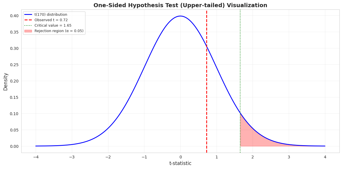
# One-sided (upper-tailed) test: H0: μ ≤ $40,000 vs Ha: μ > $40,000mu0 =40000t_stat = (mean_earnings - mu0) / se_earningsp_value_upper =1- stats.t.cdf(t_stat, n -1) # Upper tail onlyt_crit_upper = stats.t.ppf(0.95, n -1) # One-sided critical valueprint("="*70)print("ONE-SIDED HYPOTHESIS TEST (Upper-tailed)")print("="*70)print(f"H₀: μ ≤ ${mu0:,}")print(f"Hₐ: μ > ${mu0:,} (the claim we're testing)")print(f"Significance level α = 0.05")print("\nTest Results:")print(f" t-statistic: {t_stat:.4f}")print(f" p-value (upper): {p_value_upper:.4f}")print(f" Critical value: {t_crit_upper:.4f}")print("\nDecision:")print(f" p-value approach: {p_value_upper:.4f} > 0.05 → Do not reject H₀")print(f" Critical approach: {t_stat:.4f} < {t_crit_upper:.4f} → Do not reject H₀")print("\nConclusion: We do not have sufficient evidence to support the claim")print(f"that mean earnings exceed ${mu0:,}.")
======================================================================
ONE-SIDED HYPOTHESIS TEST (Upper-tailed)
======================================================================
H₀: μ ≤ $40,000
Hₐ: μ > $40,000 (the claim we're testing)
Significance level α = 0.05

Test Results:
  t-statistic:       0.7237
  p-value (upper):   0.2351
  Critical value:    1.6539

Decision:
  p-value approach:  0.2351 > 0.05 → Do not reject H₀
  Critical approach: 0.7237 < 1.6539 → Do not reject H₀

Conclusion: We do not have sufficient evidence to support the claim
that mean earnings exceed $40,000.
Visualizing One-Sided Test
# Visualize one-sided hypothesis testfig, ax = plt.subplots(figsize=(12, 6))x = np.linspace(-4, 4, 500)y = stats.t.pdf(x, n -1)# Plot the t-distributionax.plot(x, y, '-', color='#c084fc', linewidth=2, label=f't({n-1}) distribution')# Mark the observed t-statisticax.axvline(x=t_stat, color='red', linewidth=2, linestyle='--', label=f'Observed t = {t_stat:.2f}')# Mark critical value (upper tail only)ax.axvline(x=t_crit_upper, color='green', linewidth=1.5, linestyle=':', label=f'Critical value = {t_crit_upper:.2f}')# Shade rejection region (upper tail only)x_reject = x[x > t_crit_upper]ax.fill_between(x_reject, 0, stats.t.pdf(x_reject, n-1), alpha=0.3, color='red', label='Rejection region (α = 0.05)')ax.set_xlabel('t-statistic', fontsize=12)ax.set_ylabel('Density', fontsize=12)ax.set_title('One-Sided Hypothesis Test (Upper-tailed) Visualization', fontsize=14, fontweight='bold')ax.legend(fontsize=9, loc='upper left')ax.grid(True, alpha=0.3)plt.tight_layout()plt.show()print("\n📊 Interpretation:")print(f" For an upper-tailed test, we only reject H₀ if t is large and POSITIVE.")print(f" Our t-statistic ({t_stat:.2f}) is below the critical value, so we do not reject.")
📊 Interpretation:
   For an upper-tailed test, we only reject H₀ if t is large and POSITIVE.
   Our t-statistic (0.72) is below the critical value, so we do not reject.
One-Sided Test Results: H₀: μ ≤ $40,000 vs Hₐ: μ > $40,000
t-statistic: 0.7237 (same as two-sided test)
p-value (one-sided): 0.2351
p-value (two-sided): 0.4703
Critical value (one-sided, α=0.05): 1.6539
Decision: Do NOT reject H₀
Key differences from two-sided test:
p-value is exactly half:
Two-sided p-value: 0.4703
One-sided p-value: 0.2351 = 0.4703/2
Why? We only count probability in ONE tail (upper tail)
Critical value is smaller:
Two-sided critical value: ±1.9740 (5% split across two tails)
One-sided critical value: 1.6539 (5% all in one tail)
One-sided tests reject H₀ more easily in the specified direction
Directional claim:
Two-sided: “μ is different from $40,000” (could be higher OR lower)
Example: Testing if a new drug is better (not just different) than placebo
Example: Testing if a policy increases (not just changes) income
When NOT to use one-sided tests:
Avoid one-sided tests when:
You’re genuinely interested in detecting differences in either direction
You might want to detect unexpected effects
The field convention is two-sided (economics typically uses two-sided)
Warning about one-sided test abuse:
Researchers sometimes use one-sided tests to get “significant” results when two-sided tests fail. This is questionable practice:
If p (two-sided) = 0.08 → not significant at α = 0.05
If p (one-sided) = 0.04 → significant at α = 0.05
Switching to one-sided AFTER seeing the data is “p-hacking”
The choice between one-sided and two-sided should be made BEFORE collecting data
In our example:
Sample mean ($41,413) is above $40,000, consistent with Hₐ: μ > $40,000
But p-value (0.2351) > 0.05, so still not significant
The effect is too small relative to sampling variability
We cannot conclude that mean earnings exceed $40,000
Power consideration:
One advantage of one-sided tests: greater statistical power in the specified direction
If you’re only interested in detecting μ > $40,000, the one-sided test is more powerful
Trade-off: Cannot detect effects in the opposite direction
4.7 Proportions Data
The methods extend naturally to proportions (binary data).
Example: Survey data where respondents answer yes (1) or no (0).- Sample proportion: \(\hat{p} = \bar{x}\) = fraction of “yes” responses- Standard error: se(\(\hat{p}\)) = √[\(\hat{p}\)(1 - \(\hat{p}\))/n]
Confidence interval for population proportion p:\[\hat{p} \pm z_{\alpha/2} \times \sqrt{\frac{\hat{p}(1-\hat{p})}{n}}\]Note: For proportions with large n, we use the normal distribution (z) instead of t. Example: In a sample of 921 voters, 480 intend to vote Democrat. Is this different from 50%?
======================================================================
INFERENCE FOR PROPORTIONS
======================================================================
Sample size:           921
Number voting Democrat: 480
Sample proportion:     0.5212 (52.12%)
Standard error:        0.0165
95% CI:                [0.4889, 0.5534]
                        [48.89%, 55.34%]

Hypothesis Test: H₀: p = 0.50 (50-50 split)
  z-statistic:       1.2851
  p-value:           0.1988
  Decision:          Do not reject H₀

Conclusion: The proportion is NOT significantly different from 50%.
Proportion Results: 480 out of 921 voters intend to vote Democrat
Sample proportion: p̂ = 0.5212 (52.12%)
Standard error: 0.0165
95% CI: [0.4889, 0.5534] or [48.89%, 55.34%]
z-statistic (testing H₀: p = 0.50): 1.2851
p-value: 0.1988
Decision: Do NOT reject H₀
What this tells us:
We have a sample where 52.12% intend to vote Democrat. The question is: does this provide evidence that the population proportion differs from 50% (a tied race)?
Understanding the confidence interval:
The 95% CI [48.89%, 55.34%] suggests:
We’re 95% confident the true population proportion is in this range
The interval INCLUDES 50%, indicating 50-50 is plausible
The interval is fairly wide (6.45 percentage points), indicating some uncertainty
Understanding the hypothesis test:
Testing H₀: p = 0.50 (tied race) vs Hₐ: p ≠ 0.50 (one candidate ahead)
z-statistic: 1.29 (only 1.29 standard errors above 50%)
p-value: 0.1988 (about 20% chance of seeing this result if truly 50-50)
Conclusion: We cannot reject the null hypothesis of a tied race
Why use z-statistic (normal) instead of t-statistic?
For proportions with large samples (n = 921):
The sampling distribution of p̂ is approximately normal
We know the exact standard error formula: √[p̂(1-p̂)/n]
No need to estimate anything with t-distribution
Rule of thumb: Use normal approximation when np ≥ 10 and n(1-p) ≥ 10
Here: 921(0.52) = 479 and 921(0.48) = 442, both >> 10
Practical interpretation for election forecasting:
This sample shows 52% support for Democrats, but:
This is NOT statistically significant evidence of a Democratic lead (p = 0.20)
The confidence interval includes 50%, so the race could be tied
To call the race, we’d want the CI to exclude 50% entirely
How would a larger sample change things?
If we had the same proportion (52%) but with 2,500 voters instead of 921:
Standard error would shrink: √[0.52(0.48)/2500] = 0.010
95% CI would be narrower: [50.0%, 54.0%]
z-statistic would be larger: (0.52 - 0.50)/0.010 = 2.00
p-value would be smaller: 0.045 < 0.05 → significant!
Conclusion: Same proportion, but with more data, we could detect the difference
Key insight about proportions:
Proportions are just means of binary (0/1) data:
Each voter is coded as 1 (Democrat) or 0 (not Democrat)
Sample proportion = sample mean of these 0/1 values
All inference principles (SE, CI, hypothesis tests) apply identically
Key Concept 4.9: Inference for Proportions
Proportions data (like employment rates, approval ratings, or market shares) are binary variables coded as 0 or 1. All inference methods for means—confidence intervals, hypothesis tests, standard errors—extend naturally to proportions. The sample proportion \(\bar{p}\) is simply the sample mean of binary data, and the standard error formula \(se(\bar{p}) = \sqrt{\bar{p}(1-\bar{p})/n}\) follows from the variance formula for binary variables.
Key Takeaways
Core Concepts
Statistical inference lets us extrapolate from sample statistics to population parameters with quantified uncertainty.
Standard error\(\text{se}(\bar{x}) = \frac{s}{\sqrt{n}}\) measures the precision of the sample mean as an estimate of the population mean.
t-distribution is used (instead of normal) when we estimate the population standard deviation from the sample
Fatter tails than normal (accounts for extra uncertainty)
Converges to normal as \(n\) increases
Confidence intervals provide a range of plausible values
Formula: estimate \(\pm\) critical value \(\times\) standard error
One-sided tests (\(H_0: \mu \leq \mu^*\) vs \(H_a: \mu > \mu^*\), or vice versa)
Rejection region in one tail only
Use when testing a directional claim
p-value interpretation
Probability of observing data at least as extreme as ours, assuming \(H_0\) is true
Small p-value (\(< \alpha\)) → reject \(H_0\)
Common significance level: \(\alpha = 0.05\)
Methods generalize to other parameters (regression coefficients, differences in means, etc.) and proportions data
What You Learned
Statistical Concepts Covered:
Standard error and sampling distribution
t-distribution vs normal distribution
Confidence intervals (90%, 95%, 99%)
Hypothesis testing (two-sided and one-sided)
p-values and critical values
Type I error and significance level
Inference for proportions
Python Tools Used:
scipy.stats.t: t-distribution (pdf, cdf, ppf)
scipy.stats.norm: Normal distribution (for proportions)
pandas: Data manipulation
matplotlib: Visualization of hypothesis tests
Next Steps
Chapter 5: Bivariate data summary (relationships between two variables)
Chapter 6: Least squares estimator (regression foundation)
Chapter 7: Inference for regression coefficients
Congratulations!
You now understand the foundations of statistical inference:
How to quantify uncertainty using confidence intervals
How to test claims about population parameters
The difference between statistical and practical significance
When to use one-sided vs two-sided tests
These tools are fundamental to all empirical research in economics and beyond!
Practice Exercises
Test your understanding of statistical inference:
Exercise 1: Confidence Interval Interpretation
A 95% CI for mean household income is [$48,000, $56,000]
What is the point estimate (sample mean)?
What is the margin of error?
TRUE or FALSE: “There is a 95% probability that the true mean is in this interval”
TRUE or FALSE: “If we repeated sampling, 95% of CIs would contain the true mean”
Exercise 2: Standard Error Calculation
Sample of \(n=64\) observations with mean \(\$45,000\) and standard deviation \(s=\$16,000\)
Calculate the standard error
What sample size would halve the standard error?
Construct an approximate 95% CI using the “mean \(\pm\) 2SE” rule
Exercise 3: t vs z Distribution
Why do we use the t-distribution instead of the normal distribution?
For \(n=10\), find the critical value for a 95% CI
For \(n=100\), find the critical value for a 95% CI
Compare these to \(z=1.96\). What do you notice?
Exercise 4: Hypothesis Test Mechanics
Test \(H_0: \mu = 100\) vs \(H_a: \mu \neq 100\) with sample mean \(= 105\), SE \(= 3\), \(n = 49\)
Calculate the t-statistic
Find the p-value (use t-table or Python)
Make a decision at \(\alpha=0.05\)
Would your decision change if \(\alpha=0.01\)?
Exercise 5: One-Sided vs Two-Sided Tests
Sample: \(n=36\), mean \(=72\), \(s=18\)
Test \(H_0: \mu = 75\) vs \(H_a: \mu \neq 75\) (two-sided, \(\alpha=0.05\))
Test \(H_0: \mu \geq 75\) vs \(H_a: \mu < 75\) (one-sided, \(\alpha=0.05\))
Compare the p-values. What is the relationship?
In which case is the evidence against \(H_0\) stronger?
Exercise 6: Type I and Type II Errors
Define Type I error and give an example in the earnings context
Define Type II error and give an example
If we decrease \(\alpha\) from 0.05 to 0.01, what happens to the probability of Type II error?
How can we reduce both types of error simultaneously?
Exercise 7: Proportions Inference
Survey of 500 people: 275 support a policy
Calculate the sample proportion and standard error
Construct a 95% CI for the population proportion
Test \(H_0: p = 0.50\) vs \(H_a: p \neq 0.50\)
Is the result statistically significant?
Exercise 8: Python Practice
Generate a random sample of 100 observations from \(N(50, 100)\)
Calculate the 95% CI for the mean
Does the CI contain the true mean (50)?
Repeat 1000 times. What fraction of CIs contain 50?
Test \(H_0: \mu = 55\). What proportion of tests reject (should be \(\approx 0.05\))?
Case Studies
Case Study 1: Statistical Inference for Labor Productivity
Research Question: “Has global labor productivity changed significantly over time, and do productivity levels differ significantly across regions?”
This case study applies all the statistical inference methods from Chapter 4 to analyze real economic data on labor productivity across 108 countries over 25 years (1990-2014). You’ll practice:
Constructing and interpreting confidence intervals for population means
Conducting two-sided hypothesis tests to compare time periods
Performing one-sided directional tests for benchmark comparisons
Applying proportions inference to binary economic outcomes
Comparing productivity levels across regional subgroups
Interpreting results in economic context (development economics, convergence theory)
The Mendez convergence clubs dataset provides panel data on labor productivity, GDP, capital, human capital, and total factor productivity for 108 countries from 1990 to 2014.
Economic Context: Testing Convergence Hypotheses
In development economics, the convergence hypothesis suggests that poorer countries should grow faster than richer ones, leading to a narrowing of productivity gaps over time. Statistical inference allows us to test whether observed changes in productivity are:
Statistically significant (unlikely due to random sampling variation)
Economically meaningful (large enough to matter for policy)
By applying Chapter 4’s methods to this dataset, you’ll answer questions like:
Has mean global productivity increased significantly from 1990 to 2014?
Are regional productivity gaps (e.g., Africa vs. Europe) statistically significant?
What proportion of countries experienced positive productivity growth?
Can we reject specific hypotheses about productivity benchmarks?
These are real questions that economists and policymakers care about when designing development strategies.
Key Concept 4.10: Why Statistical Inference Matters in Economics
When analyzing economic data, we rarely observe entire populations. Instead, we work with samples (like 108 countries from all countries in the world, or 25 years from a longer historical period). Statistical inference lets us:
Quantify uncertainty - Confidence intervals tell us the range of plausible values for population parameters
Test theories - Hypothesis tests evaluate whether data support or contradict economic theories
Compare groups - We can determine if differences between regions/periods are real or just noise
Inform policy - Statistical significance helps separate meaningful patterns from random fluctuations
Without inference methods, we couldn’t distinguish between: - A real productivity increase vs. random year-to-year variation - Genuine regional gaps vs. sampling artifacts - Policy-relevant changes vs. statistical noise
Learning Goal: Apply hypothesis testing to compare subgroups
Economic Question: “Do African countries have significantly lower productivity than European countries (2014 data)?”
Your task:
Filter 2014 data by region (use region column in dataset)
Test H₀: μ_Africa = μ_Europe vs Hₐ: μ_Africa ≠ μ_Europe
Calculate 95% CI for the difference in means
Visualize distributions with side-by-side box plots
Code structure (complete the analysis):
# Filter 2014 data by regiondf_2014 = df.loc[df.index.get_level_values('year') ==2014]# Extract productivity for Africa and Europelp_africa = df_2014.loc[df_2014['region'] =='Africa', 'lp']lp_europe = df_2014.loc[df_2014['region'] =='Europe', 'lp']print(f"Sample sizes: Africa n={len(lp_africa)}, Europe n={len(lp_europe)}")print(f"Africa mean: ${lp_africa.mean():,.0f}")print(f"Europe mean: ${lp_europe.mean():,.0f}\n")# Conduct two-sample t-test# YOUR CODE HERE: Use stats.ttest_ind() to test if means differ# Calculate and print: t-statistic, p-value, decision at α=0.05# Calculate 95% CI for difference in means# YOUR CODE HERE: # 1. Calculate difference in means# 2. Calculate SE of difference# 3. Get t-critical value# 4. Construct CI: (difference - ME, difference + ME)# Visualize distributionsfig, ax = plt.subplots(1, 1, figsize=(8, 5))ax.boxplot([lp_africa, lp_europe], labels=['Africa', 'Europe'])ax.set_ylabel('Labor Productivity ($)')ax.set_title('Labor Productivity Distribution by Region (2014)')ax.grid(axis='y', alpha=0.3)plt.tight_layout()plt.show()
Questions to consider:
Is the difference statistically significant?
How large is the productivity gap in dollar terms?
What does the box plot reveal about within-region variation?
Does the CI for the difference include zero? What does that mean?
Key Concept 4.11: Economic vs Statistical Significance
A result can be statistically significant (p < 0.05) but economically trivial, or vice versa:
Statistical significance answers: “Is this difference unlikely to be due to chance?” - Depends on sample size: larger samples detect smaller differences - Measured by p-value: probability of observing this result if H₀ is true - Standard: p < 0.05 means <5% chance of Type I error
Economic significance answers: “Is this difference large enough to matter?” - Depends on context: a $1,000 productivity gap might be huge for low-income countries but trivial for high-income countries - Measured by effect size: actual magnitude of the difference - Judgment call: requires domain expertise
Example: - With n=10,000 countries, a $100 productivity difference might be statistically significant (p<0.001) but economically meaningless - With n=10 countries, a $10,000 difference might not be statistically significant (p=0.08) but could be economically important
Best practice: Always report BOTH: 1. Statistical result: “We reject H₀ at α=0.05 (p=0.003)” 2. Economic interpretation: “The $15,000 productivity gap represents a 35% difference, which is economically substantial for development policy”
Task 4: One-Sided Test for Growth (MORE INDEPENDENT)
Learning Goal: Apply Section 4.6 (one-sided tests) to directional hypotheses
Economic Question: “Can we conclude that mean global productivity in 2014 exceeds $50,000 (a policy benchmark)?”
Your task:
Test H₀: μ ≤ 50,000 vs Hₐ: μ > 50,000
Use scipy.stats.ttest_1samp() with alternative='greater'
Compare one-sided vs two-sided p-values
Discuss Type I error: what does α=0.05 mean in this context?
Outline (write your own code):
# Step 1: State hypotheses clearly# H₀: μ ≤ 50,000 (productivity does not exceed benchmark)# Hₐ: μ > 50,000 (productivity exceeds benchmark)# Step 2: Conduct one-sided t-test# Use: stats.ttest_1samp(lp_2014, popmean=50000, alternative='greater')# Step 3: Calculate two-sided p-value for comparison# Use: stats.ttest_1samp(lp_2014, popmean=50000, alternative='two-sided')# Step 4: Report results# - Sample mean# - t-statistic# - One-sided p-value# - Two-sided p-value# - Decision at α=0.05# Step 5: Interpret Type I error# If we reject H₀, what is the probability we made a mistake?
Hint: Remember that for one-sided tests:
If Hₐ: μ > μ₀, use alternative='greater'
The one-sided p-value is half the two-sided p-value (when t-stat has correct sign)
Type I error = rejecting H₀ when it’s actually true
Questions to consider:
Why is the one-sided p-value smaller than the two-sided p-value?
When is a one-sided test appropriate vs a two-sided test?
Learning Goal: Apply Section 4.7 (proportions) to binary outcomes
Economic Question: “What proportion of countries experienced productivity growth from 1990 to 2014, and can we conclude that more than half experienced growth?”
Your task:
Create country-level dataset with productivity in both 1990 and 2014
Learning Goal: Integrate multiple inference methods in comprehensive analysis
Economic Question: “Which regional pairs show statistically significant productivity gaps in 2014?”
Your task:
Identify all regions in the dataset (use df_2014['region'].unique())
Calculate 95% CIs for mean productivity in each region
Conduct pairwise t-tests (Africa vs Europe, Africa vs Asia, Africa vs Americas, etc.)
Create a visualization showing CIs for all regions (error bar plot)
Discuss the multiple testing problem: when conducting many tests, what happens to Type I error?
Challenge goals (minimal guidance):
Design your own analysis structure
Use loops to avoid repetitive code
Create professional visualizations
Write clear economic interpretations
Suggested approach:
# Step 1: Get all regions and calculate summary stats# For each region: mean, std, se, 95% CI# Store in a DataFrame or dictionary# Step 2: Conduct all pairwise tests# Use itertools.combinations() to generate pairs# For each pair: run ttest_ind(), store t-stat and p-value# Step 3: Visualize CIs# Create error bar plot: plt.errorbar()# Or bar plot with CI whiskers# Step 4: Report significant differences# Which pairs have p < 0.05?# What is the magnitude of differences?# Step 5: Discuss multiple testing# If you run 10 tests at α=0.05, what's the probability of at least one false positive?# Consider Bonferroni correction: α_adjusted = 0.05 / number_of_tests
Questions to consider:
Which region has the highest mean productivity? Lowest?
Are all pairwise differences statistically significant?
How does the multiple testing problem affect your conclusions?
What economic factors might explain regional productivity gaps?
What You’ve Learned
By completing this case study, you’ve practiced all the major skills from Chapter 4:
Statistical Methods:
Constructed confidence intervals (90%, 95%, 99%) for population means
Conducted two-sided hypothesis tests to compare groups and time periods
Performed one-sided directional tests for benchmark comparisons
Applied proportions inference to binary economic outcomes
Calculated and interpreted t-statistics, p-values, and margins of error
Used both manual calculations and scipy.stats functions
Economic Applications:
Tested convergence hypotheses (did productivity gaps narrow over time?)
Compared regional development levels (Africa, Europe, Asia, Americas)
These skills form the foundation for more advanced methods in later chapters:
Chapter 5: Regression analysis (relationship between two variables)
Chapter 6: Multiple regression (controlling for confounders)
Chapter 7: Hypothesis tests in regression models
Statistical inference is everywhere in empirical economics. You’ve now mastered the core toolkit for:
Quantifying uncertainty
Testing economic theories
Making data-driven decisions
Communicating results with precision
Well done!
Case Study 2: Is Bolivia’s Development Equal? Testing Differences Across Departments
Research Question: Are there statistically significant differences in development levels across Bolivia’s nine departments?
In Chapter 1, we introduced the DS4Bolivia project and explored satellite-development relationships across Bolivia’s 339 municipalities. In this case study, we apply Chapter 4’s statistical inference tools—confidence intervals and hypothesis tests—to test whether development levels differ significantly across Bolivia’s departments.
The Data: Cross-sectional dataset covering 339 Bolivian municipalities from the DS4Bolivia Project, including:
Development outcomes: Municipal Sustainable Development Index (IMDS, 0-100 composite)
Satellite data: Log nighttime lights per capita (2017)
Demographics: Population (2017), municipality and department names
Your Task: Use confidence intervals, one-sample tests, two-sample tests, and one-sided tests to evaluate whether Bolivia’s departments differ significantly in development—and whether those differences are large enough to matter for policy.
Load the DS4Bolivia Data
Let’s load the DS4Bolivia dataset and prepare the key variables for statistical inference.
# Load the DS4Bolivia dataseturl_bol ="https://raw.githubusercontent.com/quarcs-lab/ds4bolivia/master/ds4bolivia_v20250523.csv"bol = pd.read_csv(url_bol)# Select key variables for this case studykey_vars = ['mun', 'dep', 'imds', 'ln_NTLpc2017', 'pop2017']bol_key = bol[key_vars].dropna().copy()print("="*70)print("DS4BOLIVIA DATASET — STATISTICAL INFERENCE CASE STUDY")print("="*70)print(f"Municipalities: {len(bol_key)}")print(f"Departments: {bol_key['dep'].nunique()}")print(f"\nIMDS summary:")print(bol_key['imds'].describe().round(2))print(f"\nMunicipalities per department:")print(bol_key['dep'].value_counts().sort_index())
======================================================================
DS4BOLIVIA DATASET — STATISTICAL INFERENCE CASE STUDY
======================================================================
Municipalities: 333
Departments:    9

IMDS summary:
count    333.00
mean      51.16
std        6.76
min       35.70
25%       47.10
50%       50.80
75%       55.00
max       80.20
Name: imds, dtype: float64

Municipalities per department:
dep
Beni          18
Chuquisaca    29
Cochabamba    47
La Paz        87
Oruro         35
Pando         13
Potosí        38
Santa Cruz    55
Tarija        11
Name: count, dtype: int64
Task 1: Confidence Interval for Mean IMDS (Guided)
Learning Goal: Apply Section 4.3 methods to calculate and interpret a confidence interval for a population mean.
Economic Question: “What is the true average development level across all Bolivian municipalities?”
Instructions:
Calculate the sample mean and standard error of imds
Construct a 95% confidence interval using scipy.stats.t.interval()
Print the sample mean, standard error, and CI bounds
Interpret the result: “We are 95% confident that the true mean municipal development index lies between X and Y.”
Apply what you learned in Section 4.3: The formula is \(\bar{x} \pm t_{\alpha/2} \times SE\), where \(SE = s/\sqrt{n}\).
# Your code here: 95% Confidence Interval for national mean IMDSfrom scipy import stats# Calculate sample statisticsn =len(bol_key['imds'])x_bar = bol_key['imds'].mean()se = bol_key['imds'].std() / np.sqrt(n)# 95% confidence interval using t-distributionci_low, ci_high = stats.t.interval(0.95, df=n-1, loc=x_bar, scale=se)print("="*70)print("95% CONFIDENCE INTERVAL FOR MEAN IMDS")print("="*70)print(f"Sample size (n): {n}")print(f"Sample mean: {x_bar:.4f}")print(f"Standard error: {se:.4f}")print(f"95% CI: [{ci_low:.4f}, {ci_high:.4f}]")print(f"\nInterpretation: We are 95% confident that the true mean")print(f"municipal development index lies between {ci_low:.2f} and {ci_high:.2f}.")
======================================================================
95% CONFIDENCE INTERVAL FOR MEAN IMDS
======================================================================
Sample size (n):       333
Sample mean:           51.1580
Standard error:        0.3704
95% CI:                [50.4292, 51.8867]

Interpretation: We are 95% confident that the true mean
municipal development index lies between 50.43 and 51.89.
Task 2: Hypothesis Test — National Development Target (Guided)
Learning Goal: Apply Section 4.4 (two-sided test) to test a hypothesis about a population mean.
Economic Question: “Is the average municipality at the midpoint of the development scale?”
A natural benchmark for the IMDS (which ranges from 0 to 100) is the midpoint of 50. If Bolivia’s municipalities were, on average, at this midpoint, we would expect \(\mu_{IMDS} = 50\).
Instructions:
State the hypotheses: \(H_0: \mu = 50\) vs \(H_1: \mu \neq 50\)
Use scipy.stats.ttest_1samp() to conduct the test
Report the t-statistic and p-value
State your conclusion at \(\alpha = 0.05\)
Discuss: Is the average municipality at the midpoint of the development scale?
# Your code here: One-sample t-test — is mean IMDS = 50?# Hypothesis test: H0: mu = 50 vs H1: mu != 50t_stat, p_value = stats.ttest_1samp(bol_key['imds'], popmean=50)print("="*70)print("HYPOTHESIS TEST: IS MEAN IMDS = 50?")print("="*70)print(f"H₀: μ = 50 vs H₁: μ ≠ 50")print(f"\nSample mean: {bol_key['imds'].mean():.4f}")print(f"t-statistic: {t_stat:.4f}")print(f"p-value: {p_value:.6f}")print(f"\nConclusion at α = 0.05:")if p_value <0.05:print(f" Reject H₀ (p = {p_value:.6f} < 0.05)")print(f" The average IMDS is significantly different from 50.")else:print(f" Fail to reject H₀ (p = {p_value:.6f} ≥ 0.05)")print(f" No significant evidence that mean IMDS differs from 50.")
======================================================================
HYPOTHESIS TEST: IS MEAN IMDS = 50?
======================================================================
H₀: μ = 50  vs  H₁: μ ≠ 50

Sample mean:   51.1580
t-statistic:   3.1258
p-value:       0.001929

Conclusion at α = 0.05:
  Reject H₀ (p = 0.001929 < 0.05)
  The average IMDS is significantly different from 50.
Key Concept 4.12: Statistical Significance in Development
A statistically significant difference between departments does not automatically imply a policy-relevant gap. With 339 municipalities providing large sample sizes, even small differences can achieve statistical significance. Policy makers must evaluate the magnitude of differences alongside p-values. A 2-point difference in IMDS may be statistically significant but practically negligible for resource allocation decisions.
Task 3: Department-Level Inference (Semi-guided)
Learning Goal: Apply confidence intervals to compare subgroups.
Economic Question: “Which departments have significantly different development levels from one another?”
Instructions:
Calculate the 95% confidence interval for mean imds in each of Bolivia’s 9 departments
Create a forest plot (horizontal error bars) showing the CI for each department
Identify which departments’ CIs overlap (suggesting no significant difference) and which don’t
Discuss what the pattern reveals about regional inequality
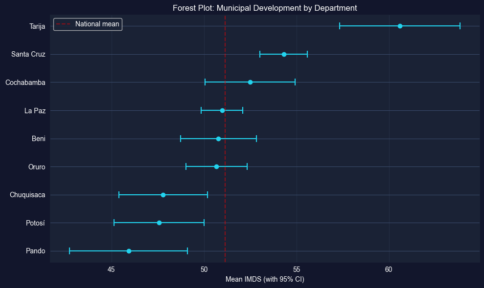
Hint: Use groupby('dep') to calculate department-level statistics, then plt.errorbar() or plt.barh() with error bars for the forest plot.
# Your code here: Department-level 95% CIs and forest plot# Calculate department-level statisticsdept_stats = bol_key.groupby('dep')['imds'].agg(['mean', 'std', 'count']).sort_values('mean')dept_stats['se'] = dept_stats['std'] / np.sqrt(dept_stats['count'])dept_stats['ci_low'] = dept_stats['mean'] -1.96* dept_stats['se']dept_stats['ci_high'] = dept_stats['mean'] +1.96* dept_stats['se']print("="*70)print("95% CONFIDENCE INTERVALS FOR MEAN IMDS BY DEPARTMENT")print("="*70)print(dept_stats[['mean', 'se', 'ci_low', 'ci_high', 'count']].round(2).to_string())# Forest plotfig, ax = plt.subplots(figsize=(10, 6))departments = dept_stats.indexy_pos =range(len(departments))ax.errorbar(dept_stats['mean'], y_pos, xerr=1.96* dept_stats['se'], fmt='o', color='#22d3ee', capsize=5, capthick=1.5, markersize=6)ax.set_yticks(y_pos)ax.set_yticklabels(departments)ax.set_xlabel('Mean IMDS (with 95% CI)')ax.set_title('Forest Plot: Municipal Development by Department')ax.axvline(x=bol_key['imds'].mean(), color='red', linestyle='--', alpha=0.5, label='National mean')ax.legend()ax.grid(axis='x', alpha=0.3)plt.tight_layout()plt.show()
======================================================================
95% CONFIDENCE INTERVALS FOR MEAN IMDS BY DEPARTMENT
======================================================================
             mean    se  ci_low  ci_high  count
dep
Pando       45.92  1.62   42.74    49.10     13
Potosí      47.57  1.24   45.14    50.01     38
Chuquisaca  47.80  1.23   45.39    50.20     29
Oruro       50.68  0.85   49.02    52.35     35
Beni        50.79  1.04   48.75    52.83     18
La Paz      50.98  0.58   49.85    52.11     87
Cochabamba  52.50  1.24   50.07    54.93     47
Santa Cruz  54.31  0.65   53.04    55.59     55
Tarija      60.60  1.66   57.35    63.85     11
Task 4: One-Sided Test — Is the Capital Department More Developed? (Semi-guided)
Learning Goal: Apply Section 4.6 (one-sided tests) to a directional hypothesis.
Economic Question: “Is La Paz department’s mean IMDS significantly greater than the national mean?”
Instructions:
Extract IMDS values for La Paz department
Test \(H_0: \mu_{LP} \leq \mu_{national}\) vs \(H_1: \mu_{LP} > \mu_{national}\) using a one-sided t-test
Calculate the one-sided p-value (divide the two-sided p-value by 2, checking direction)
Report and interpret the result at \(\alpha = 0.05\)
Discuss: Is the capital department significantly more developed?
Hint: Use scipy.stats.ttest_1samp() with the national mean as the test value, then adjust for a one-sided test.
# Your code here: One-sided t-test for La Paz department# Extract La Paz IMDS valuesla_paz = bol_key[bol_key['dep'] =='La Paz']['imds']national_mean = bol_key['imds'].mean()# Two-sided test firstt_stat_lp, p_two = stats.ttest_1samp(la_paz, popmean=national_mean)# One-sided p-value: H1: mu_LP > national_mean# If t > 0, one-sided p = p_two / 2; if t < 0, one-sided p = 1 - p_two / 2p_one = p_two /2if t_stat_lp >0else1- p_two /2print("="*70)print("ONE-SIDED TEST: LA PAZ > NATIONAL MEAN?")print("="*70)print(f"H₀: μ_LaPaz ≤ {national_mean:.2f} vs H₁: μ_LaPaz > {national_mean:.2f}")print(f"\nLa Paz municipalities: {len(la_paz)}")print(f"La Paz mean IMDS: {la_paz.mean():.4f}")print(f"National mean IMDS: {national_mean:.4f}")print(f"t-statistic: {t_stat_lp:.4f}")print(f"One-sided p-value: {p_one:.6f}")print(f"\nConclusion at α = 0.05:")if p_one <0.05:print(f" Reject H₀ (p = {p_one:.6f} < 0.05)")print(f" La Paz's mean IMDS is significantly greater than the national mean.")else:print(f" Fail to reject H₀ (p = {p_one:.6f} ≥ 0.05)")print(f" No significant evidence that La Paz exceeds the national mean.")
======================================================================
ONE-SIDED TEST: LA PAZ > NATIONAL MEAN?
======================================================================
H₀: μ_LaPaz ≤ 51.16  vs  H₁: μ_LaPaz > 51.16

La Paz municipalities:  87
La Paz mean IMDS:       50.9782
National mean IMDS:     51.1580
t-statistic:            -0.3120
One-sided p-value:      0.622110

Conclusion at α = 0.05:
  Fail to reject H₀ (p = 0.622110 ≥ 0.05)
  No significant evidence that La Paz exceeds the national mean.
When testing hypotheses about departmental means, each department contains a different number of municipalities (ranging from ~10 to ~50+). Departments with fewer municipalities have wider confidence intervals and less statistical power. This means we may fail to detect real differences for smaller departments—not because the differences don’t exist, but because we lack sufficient data to establish them conclusively.
Task 5: Comparing Two Departments (Independent)
Learning Goal: Apply two-sample t-tests to compare group means.
Economic Question: “Is the development gap between the most and least developed departments statistically significant?”
Instructions:
Identify the departments with the highest and lowest mean IMDS (from Task 3 results)
Use scipy.stats.ttest_ind() to perform a two-sample t-test comparing these departments
Report the t-statistic and p-value
Discuss both statistical significance (p-value) and practical significance (magnitude of the gap)
What does this tell us about regional inequality in Bolivia?
# Your code here: Two-sample t-test — highest vs lowest IMDS department# Identify highest and lowest departmentsdept_means = bol_key.groupby('dep')['imds'].mean()top_dept = dept_means.idxmax()bot_dept = dept_means.idxmin()# Extract IMDS values for eachtop_values = bol_key[bol_key['dep'] == top_dept]['imds']bot_values = bol_key[bol_key['dep'] == bot_dept]['imds']# Two-sample t-testt_stat_2s, p_value_2s = stats.ttest_ind(top_values, bot_values)print("="*70)print(f"TWO-SAMPLE T-TEST: {top_dept.upper()} vs {bot_dept.upper()}")print("="*70)print(f"\nHighest IMDS department: {top_dept}")print(f" Mean IMDS: {top_values.mean():.4f}")print(f" N: {len(top_values)}")print(f"\nLowest IMDS department: {bot_dept}")print(f" Mean IMDS: {bot_values.mean():.4f}")print(f" N: {len(bot_values)}")print(f"\nDifference in means: {top_values.mean() - bot_values.mean():.4f}")print(f"t-statistic: {t_stat_2s:.4f}")print(f"p-value: {p_value_2s:.6f}")print(f"\nConclusion at α = 0.05:")if p_value_2s <0.05:print(f" Reject H₀ (p = {p_value_2s:.6f} < 0.05)")print(f" The development gap of {top_values.mean() - bot_values.mean():.2f} points is statistically significant.")else:print(f" Fail to reject H₀ (p = {p_value_2s:.6f} ≥ 0.05)")print(f" No significant evidence of a development gap.")print(f"\nPractical significance: A gap of {top_values.mean() - bot_values.mean():.2f} points on a 0-100 scale")print(f"represents a {'substantial'ifabs(top_values.mean() - bot_values.mean()) >10else'modest'} difference in development outcomes.")
======================================================================
TWO-SAMPLE T-TEST: TARIJA vs PANDO
======================================================================

Highest IMDS department: Tarija
  Mean IMDS:   60.6000
  N:           11

Lowest IMDS department:  Pando
  Mean IMDS:   45.9231
  N:           13

Difference in means:    14.6769
t-statistic:            6.2916
p-value:                0.000002

Conclusion at α = 0.05:
  Reject H₀ (p = 0.000002 < 0.05)
  The development gap of 14.68 points is statistically significant.

Practical significance: A gap of 14.68 points on a 0-100 scale
represents a substantial difference in development outcomes.
Task 6: Policy Brief on Regional Inequality (Independent)
Objective: Write a 200-300 word policy brief summarizing your statistical findings.
Your brief should address:
Are departmental differences statistically significant? Summarize results from Tasks 3-5.
Which departments need the most attention? Use the forest plot and CI analysis to identify lagging regions.
How confident are we in these conclusions? Discuss the confidence levels and what the CIs tell us.
What are the limitations of these tests? Consider sample sizes, assumptions, and what the tests cannot tell us.
Format: Write your brief in the markdown cell below. Support your arguments with specific numbers from your analysis (means, CIs, p-values).
Tip: Remember Key Concepts 4.12 and 4.13—distinguish between statistical significance and policy relevance, and consider how unequal sample sizes affect your conclusions.
# Your code here: Additional analysis to support your policy brief## Suggestions:# 1. Create a summary table of all department CIs and test results# 2. Calculate effect sizes (Cohen's d) for the two-sample comparison# 3. Visualize the national IMDS distribution with department means marked# Example: Summary statistics for the policy briefprint("="*70)print("SUMMARY TABLE FOR POLICY BRIEF")print("="*70)dept_summary = bol_key.groupby('dep')['imds'].agg(['mean', 'std', 'count']).sort_values('mean', ascending=False)dept_summary['se'] = dept_summary['std'] / np.sqrt(dept_summary['count'])dept_summary['ci_95'] = dept_summary.apply(lambda r: f"[{r['mean'] -1.96*r['se']:.1f}, {r['mean'] +1.96*r['se']:.1f}]", axis=1)print(dept_summary[['mean', 'std', 'count', 'ci_95']].round(2).to_string())
Through this analysis of subnational development in Bolivia, you’ve applied the full Chapter 4 statistical inference toolkit:
Confidence intervals for mean development levels
One-sample and two-sample hypothesis tests to evaluate development benchmarks and compare groups
One-sided tests for directional hypotheses about specific departments
Forest plots for comparing group CIs visually
Statistical vs practical significance in a policy context
Critical thinking about sample size, statistical power, and inference limitations
Connection to research: The DS4Bolivia project uses these same statistical tools to evaluate whether satellite-predicted development indicators are significantly different from survey-based measures, providing evidence for the reliability of remote sensing approaches to SDG monitoring.
Looking ahead: In Chapter 5, we’ll move beyond testing means to exploring bivariate relationships—how nighttime lights relate to specific development outcomes across Bolivia’s municipalities.
Well done! You’ve now tested development hypotheses for both cross-country convergence and Bolivian regional inequality using the tools of statistical inference.