import warnings
from pathlib import Path

import matplotlib.pyplot as plt
import numpy as np
import pandas as pd

from scspill import SCSPILL
from scspill.data import load_california, load_california_cd

warnings.filterwarnings("ignore", category=RuntimeWarning)
root = Path.cwd()
while not (root / "benchmarks").exists():   # docs pages execute in docs/articles
    root = root.parent
MCMC = {"m_iter": 4000, "burn": 2000, "seed": 42, "display_graphs": False}The cd model in practice
Usage, the Proposition 99 results, and where the answers disagree
This article is for readers who want to use the cd model and to know how far to trust what it says. It shows the essential usage, the model’s main results on Proposition 99, and four places where the answer depends on a choice:
- the model itself (
cdagainstsar); - the inference rule (the paper’s against the authors’ code);
- the assumed exposure structure (which the data reject);
- the statistic used to choose a structure (scspill’s against mlsynth’s).
The main text stays plain. The formal details sit in the collapsed callouts. The Proposition 99 case study is the hands-on tutorial this article builds on.
NoteMCMC budget
The sar fits on this page run a tutorial-scale chain (m_iter=4000, burn=2000) so the page renders in minutes. Treat their numbers as illustrative, and use tens of thousands of iterations for real work. The cd fits involve no simulation.
Using cd
A fit needs a long panel with a 0/1 treatment column, and a statement of which controls the treatment can reach. Everything else has a default.
panel = load_california_cd(51)          # 50 states + DC, California treated from 1989
cd51 = SCSPILL({**panel.config_kwargs(), "display_graphs": False}).fit()
panel.config_kwargs() fills in method="cd", the column names, and the paper’s 13 exposed states. With your own data you write the dictionary yourself:
SCSPILL({
    "method": "cd", "df": df, "outcome": "y", "treat": "treated",
    "unitid": "unit", "time": "year",
    "affected_units": ["NV", "AZ"],              # per-unit spillovers (default)
    # "spillover_structure": "homogeneous",      # one shared spillover
    # "spillover_structure": "distance_decay", "unit_distances": {"NV": 0.5},
    # "spillover_structure": "custom", "effect_matrix": A,
}).fit()| Question | Accessor |
|---|---|
| What is the effect on the treated unit? | att, effects_panel["CA"], effect_ci["CA"] |
| Did the treatment spill over, and onto whom? | effects_panel[unit], pointwise_p_values, test_hypothesis(C) |
| Is the assumed structure right? | kappa_test, select_structure_by_kappa(candidates) |
| How much could a missed spillover bias the result? | cd.sensitivity, plot(kind="sensitivity") |
TipFormal details: the estimator and the test
Every unit \(i\) gets an intercept \(\hat a_i\) and simplex weights \(\hat b_i\) on the other units, fitted before treatment. With \(R = I - \hat B\), the post-treatment equations \(R Y_t - \hat a = R A \gamma_t + u_t\) give \(\hat\gamma_t = (A'R'RA)^{-1}A'R'(RY_t - \hat a)\) and \(\hat\alpha_t = A\hat\gamma_t\) (Cao & Dowd v3, Section 3.2). A hypothesis \(C\alpha_t = d\) is tested by \(P = (C\hat\alpha_t - d)'W(C\hat\alpha_t - d)\), compared with the same quadratic form on the \(T_0\) pre-treatment placebo effects \(\hat G\hat u_s\), \(\hat G = A(A'R'RA)^{-1}A'R'\). The test rejects above the left inverse of their empirical CDF at \(1-\tau\) (Section 4.2), and intervals invert that test.
The main results
The direct effect. Proposition 99 lowered California’s consumption, but not at once:
ca = cd51.effect_ci["CA"].assign(
    estimate=cd51.effects_panel["CA"], p_value=cd51.pointwise_p_values["CA"]
)
ca.round(2).T| 1989 | 1990 | 1991 | 1992 | 1993 | 1994 | 1995 | 1996 | 1997 | 1998 | 1999 | 2000 | |
|---|---|---|---|---|---|---|---|---|---|---|---|---|
| lower | -4.64 | -1.00 | -8.48 | -8.15 | -12.33 | -15.63 | -17.55 | -17.80 | -19.63 | -20.80 | -23.68 | -20.21 |
| upper | 4.80 | 8.43 | 0.96 | 1.29 | -2.90 | -6.19 | -8.12 | -8.37 | -10.19 | -11.36 | -14.24 | -10.77 |
| estimate | 0.08 | 3.71 | -3.76 | -3.43 | -7.61 | -10.91 | -12.83 | -13.08 | -14.91 | -16.08 | -18.96 | -15.49 |
| p_value | 1.00 | 0.05 | 0.05 | 0.05 | 0.00 | 0.00 | 0.00 | 0.00 | 0.00 | 0.00 | 0.00 | 0.00 |
cd51.plot(kind="spillover", display=False);findfont: Failed to find font weight medium, now using 400.
findfont: Failed to find font weight medium, now using 400.
findfont: Failed to find font weight medium, now using 400.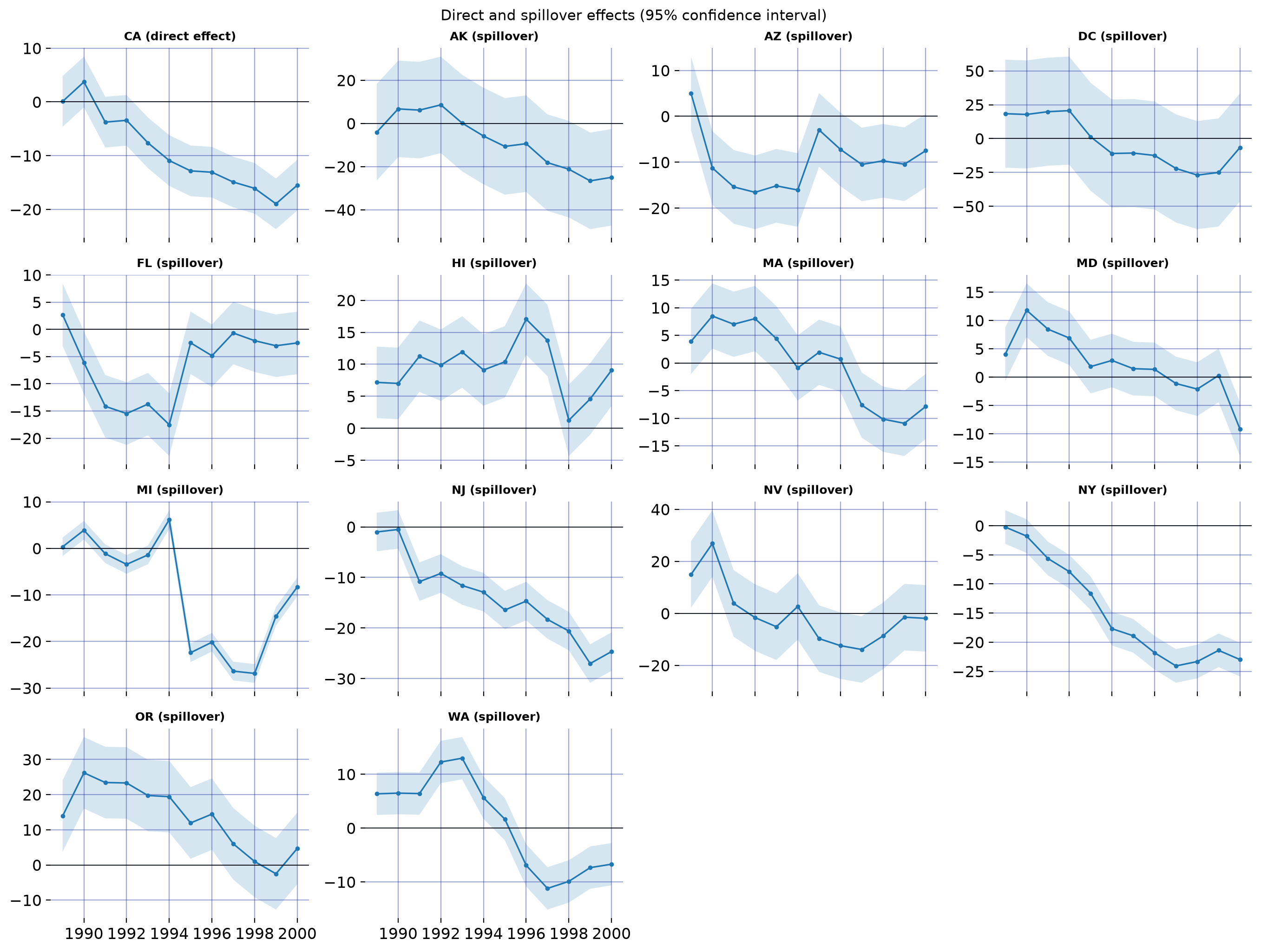
The intervals cover zero from 1989 to 1992 and exclude it from 1993. The average over 1989–2000 is -9.4 packs per capita. California’s own synthetic control, which ignores spillovers, gives -10.8.
Spillovers. Nevada, the neighbour with no tobacco law of its own, shows leakage: its consumption rises in the first two years and then fades. Whether any exposed state was affected is one joint test per year:
no_spillover = np.eye(len(cd51.unit_labels))[1:]   # every unit but California
joint = pd.DataFrame(
    {
        t: {"p_value": f"{cd51.test_hypothesis(no_spillover, period=t).p_value:.3f}",
            "reject": cd51.test_hypothesis(no_spillover, period=t).reject}
        for t in cd51.effects_panel.index
    }
)
joint| 1989 | 1990 | 1991 | 1992 | 1993 | 1994 | 1995 | 1996 | 1997 | 1998 | 1999 | 2000 | |
|---|---|---|---|---|---|---|---|---|---|---|---|---|
| p_value | 0.263 | 0.000 | 0.000 | 0.000 | 0.105 | 0.053 | 0.053 | 0.000 | 0.000 | 0.000 | 0.000 | 0.000 |
| reject | False | True | True | True | False | False | False | True | True | True | True | True |
Robustness to missed spillovers. If one assumed-clean state in fact received a spillover, how large would it have to be to account for California’s largest estimate? The answer is the paper’s Figure 3:
sens = cd51.cd.sensitivity
largest = cd51.effects_panel["CA"].max()
pd.DataFrame(
    {f"{p} missed": {"spillover-aware": largest / sens.coefficients(p)[0],
                     "pure-donor SCM": largest / sens.coefficients(p)[1]}
     for p in (1, 2)}
).round(2)| 1 missed | 2 missed | |
|---|---|---|
| spillover-aware | 17.07 | 9.66 |
| pure-donor SCM | 6.73 | 5.33 |
Dropping the exposed states and using only clean donors would be far more fragile: a smaller missed spillover suffices to explain the estimate away.
Disagreement 1: cd against sar — model or sample?
On their default samples the two models disagree twice:
- on the size of California’s effect;
- on the sign of Nevada’s spillover.
But they also differ in sample:
sar’s bundled panel is Abadie et al.’s 39 states, with sales measured from 1988;cd’s is Cao & Dowd’s 51 units, with consumption measured from 1989.
To separate the model from the sample, fit both models on all three samples:
cdon the 39-state panel, with Nevada as the exposed state (it is California’s only neighbour in that sample);saron the 51- and 41-unit panels, with rook-contiguity weights built from the same Census source and rule as the bundled ones (seedocs/articles/data/README.txtin the repository).
W = pd.read_csv(root / "docs" / "articles" / "data" / "cd_rook_W.csv", index_col="state")
adh = load_california()
fits = {
    ("cd", "39 states (1988)"): SCSPILL(
        {**adh.config_kwargs(method="cd"), "affected_units": ["Nevada"], "display_graphs": False}
    ).fit(),
    ("sar", "39 states (1988)"): SCSPILL({**adh.config_kwargs(), **MCMC}).fit(),
}
for spec in (51, 41):
    cdp = load_california_cd(spec)
    donors = sorted(set(cdp.df["state"]) - {"CA"})
    label = f"{spec} units (1989)"
    fits[("cd", label)] = SCSPILL({**cdp.config_kwargs(), "display_graphs": False}).fit()
    fits[("sar", label)] = SCSPILL(
        {"df": cdp.df, "outcome": "cigs", "treat": "treated", "unitid": "state",
         "time": "year", "spatial_w": W.loc["CA", donors],
         "spatial_W": W.loc[donors, donors], **MCMC}
    ).fit()


def nevada(model, fit):
    label = "Nevada" if "Nevada" in fit.inputs.control_labels else "NV"
    if model == "cd":
        return fit.effects_panel[label].iloc[:2].to_numpy()
    return fit.spillover_panel[label].loc[fit.inputs.time_post].iloc[:2].to_numpy()


grid = pd.DataFrame(
    {
        key: {
            "ATT on California": fit.att,
            "ATT, no-spillover SCM": fit.att_scm,
            "Nevada, 1st year": nevada(key[0], fit)[0],
            "Nevada, 2nd year": nevada(key[0], fit)[1],
            "rho (sar)": fit.rho_hat if key[0] == "sar" else np.nan,
        }
        for key, fit in fits.items()
    }
).T
grid.round(2)| ATT on California | ATT, no-spillover SCM | Nevada, 1st year | Nevada, 2nd year | rho (sar) | ||
|---|---|---|---|---|---|---|
| cd | 39 states (1988) | -2.77 | -10.52 | 22.74 | 25.44 | NaN |
| sar | 39 states (1988) | -17.07 | -15.70 | -2.18 | -3.45 | 0.37 |
| cd | 51 units (1989) | -9.44 | -10.81 | 14.96 | 26.86 | NaN |
| sar | 51 units (1989) | -15.49 | -14.68 | -1.00 | -1.18 | 0.38 |
| cd | 41 units (1989) | -10.06 | -13.02 | 22.46 | 38.20 | NaN |
| sar | 41 units (1989) | -14.84 | -14.43 | -0.51 | -0.66 | 0.24 |
fig, axes = plt.subplots(1, 2, figsize=(11, 4), sharey=True)
for ax, model in zip(axes, ("cd", "sar")):
    for (m, sample), fit in fits.items():
        if m != model:
            continue
        t0 = fit.inputs.T0
        years = fit.inputs.time_labels[t0:]
        ax.plot(years, fit.gap[t0:], marker="o", markersize=3, label=sample)
    ax.axhline(0, color="black", linewidth=0.8)
    ax.set_title(f"{model}")
    ax.set_xlabel("Year")
axes[0].set_ylabel("Effect on California (packs per capita)")
axes[0].legend(fontsize=8);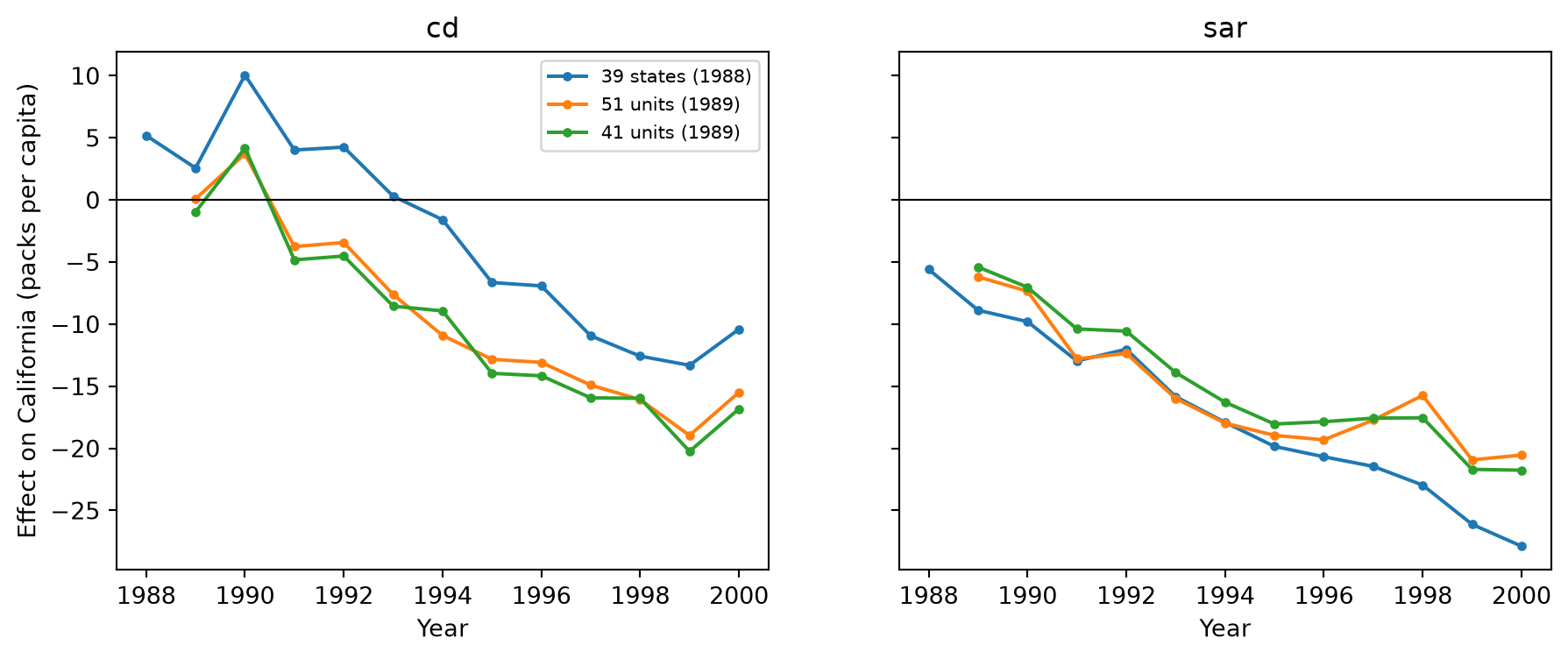
Reading the grid down the columns holds the sample fixed and changes the model. Reading along the rows holds the model fixed and changes the sample.
- The sign of Nevada’s spillover is the model’s. On every sample
cdfinds Nevada’s consumption rising after 1989, andsarfinds it falling slightly. - The size of California’s effect depends on both.
sarputs it near −15 to −17 packs on every sample.cdputs it nearer −10 on the Cao–Dowd samples, and much closer to zero on the 39-state panel, where Nevada is the only exposed state and absorbs a large leakage.
The mechanism is the models’ assumptions, not noise.
cdestimates a separate, unrestricted effect for every exposed state, so leakage shows up as a positive spillover on Nevada. California’s counterfactual is built from the donors’ untreated outcomes, so removing Nevada’s leakage lowers the counterfactual by Nevada’s weight times the leakage, which pulls California’s direct effect toward zero. That weight is what makes the samples differ:
pd.Series(
    {
        "39 states (1988)": fits[("cd", "39 states (1988)")].scm_matrix.loc["California", "Nevada"],
        "51 units (1989)": fits[("cd", "51 units (1989)")].scm_matrix.loc["CA", "NV"],
        "41 units (1989)": fits[("cd", "41 units (1989)")].scm_matrix.loc["CA", "NV"],
    },
    name="Nevada's weight in California's synthetic control",
).round(3)
39 states (1988) 0.247
51 units (1989) 0.069
41 units (1989) 0.164
Name: Nevada's weight in California's synthetic control, dtype: float64On the 39-state panel Nevada carries a quarter of California’s synthetic control. Its large leakage therefore moves California’s estimate most there.
sarlets the treated unit’s outcome propagate to its neighbours through one intensity \(\rho\). With \(\rho > 0\), a fall in California is passed on as a fall in Nevada. The model cannot produce leakage, which moves Nevada the other way, unless \(\rho\) turns negative for every channel at once, and the data put \(\rho\) above zero on all three samples.
TipFormal details: the sign of
sar’s spillover
In sar, donor outcomes follow \(\mathbf Y^c_t = \rho(\mathbf w Y_{0t} +
\mathbf W \mathbf Y^c_t) + \dots\). Its identification result implies that the spillover vector is exactly \[
\boldsymbol\xi^c_t = (\mathbf I - \rho\mathbf A)^{-1}\rho\,\mathbf w\,
\bigl(Y_{0t} - \boldsymbol\alpha^\top \mathbf Y^c_t\bigr),
\qquad \mathbf A = \mathbf W + \mathbf w\boldsymbol\alpha^\top ,
\] the treated unit’s observed gap propagated through the network. For small \(\rho\), \((\mathbf I - \rho\mathbf A)^{-1} \approx \mathbf I\), so Nevada’s spillover is about \(\rho\, w_{\text{NV}}\) times California’s gap: it has the sign of \(\rho\) times California’s change. In cd, \(\alpha_{\text{NV},t}\) is a free parameter of \(\gamma_t\); nothing ties its sign to \(\alpha_{\text{CA},t}\).
Neither model is “right”. They encode different beliefs about how the policy travels. Run both: where they agree, as on a clearly negative effect from the mid-1990s, the conclusion does not hinge on the spillover assumption; where they disagree, as on Nevada, it does.
Disagreement 3: the data reject the assumed structure
The \(\kappa_A\) test asks whether the part of the post-treatment residuals that the 13-state structure cannot explain looks like the pre-treatment residuals. It does not:
cd51.plot(kind="kappa", display=False);findfont: Failed to find font weight medium, now using 400.
findfont: Failed to find font weight medium, now using 400.
findfont: Failed to find font weight medium, now using 400.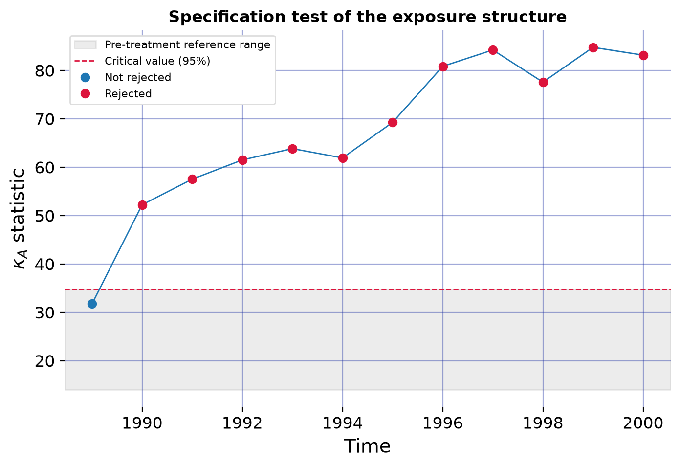
A rejection says something moved after 1989 that the structure does not capture. It does not say what. Three checks narrow it down.
Which states carry the unexplained part? Split the unexplained residual by state, after 1989 and, for comparison, before:
from scspill.utils.scspill_helpers.cd.estimation import effect_operator

labels = list(cd51.unit_labels)
B = cd51.scm_matrix.loc[labels, labels].to_numpy()
a = cd51.intercepts[labels].to_numpy()
op = effect_operator(B, cd51.effect_matrix.to_numpy())
R = np.eye(len(labels)) - B
Y, t0 = cd51.inputs.Y_units, cd51.inputs.T0
unexplained = lambda block: (np.eye(len(labels)) - op.projector) @ (R @ block - a[:, None])
post = pd.Series((unexplained(Y[:, t0:]) ** 2).sum(axis=1), index=labels)
pre = pd.Series((unexplained(Y[:, :t0]) ** 2).sum(axis=1), index=labels)
shares = pd.DataFrame({"share after 1989": post / post.sum(), "share before 1989": pre / pre.sum()})
shares.sort_values("share after 1989", ascending=False).head(8).round(3)| share after 1989 | share before 1989 | |
|---|---|---|
| NH | 0.121 | 0.240 |
| KY | 0.083 | 0.154 |
| RI | 0.067 | 0.021 |
| WV | 0.062 | 0.011 |
| VT | 0.061 | 0.012 |
| TX | 0.060 | 0.006 |
| IN | 0.056 | 0.028 |
| VA | 0.052 | 0.001 |
The unexplained part is spread over many states, led by a handful of unexposed ones. The two largest contributors after 1989 were also among the hardest to fit before it.
Does a larger structure fix it? Add the leading contributors to the exposed set and refit:
top = [u for u in shares["share after 1989"].sort_values(ascending=False).index
       if u not in cd51.inputs.affected_labels and u != "CA"]
paper_set = list(cd51.inputs.affected_labels)
rows = {}
for name, extra in {"paper (13)": [], "+ top 3": top[:3], "+ top 5": top[:5]}.items():
    fit = SCSPILL({**panel.config_kwargs(), "affected_units": paper_set + extra,
                   "display_graphs": False}).fit()
    stats = [k.statistic for k in fit.kappa_test.values()]
    rows[name] = {
        "added": ", ".join(extra) or "-",
        "mean kappa_A": f"{np.mean(stats):.1f}",
        "years rejected": sum(k.reject for k in fit.kappa_test.values()),
        "ATT on California": f"{fit.att:.2f}",
    }
pd.DataFrame(rows).T| added | mean kappa_A | years rejected | ATT on California | |
|---|---|---|---|---|
| paper (13) | - | 67.4 | 11 | -9.44 |
| + top 3 | NH, KY, RI | 50.5 | 11 | -16.14 |
| + top 5 | NH, KY, RI, WV, VT | 48.0 | 11 | -15.58 |
Adding them lowers the statistic but not the verdict, and it moves California’s estimated effect substantially. The direct effect is sensitive to which states the analyst declares exposed. That is the misspecification bias of Section 5.1.1 made visible.
Is it the reference distribution? Full-sample references come from fitted residuals, which are smaller than out-of-sample ones. Leave-one-out references raise the critical value:
loo = SCSPILL({**panel.config_kwargs(), "reference_mode": "leave_one_period_out",
               "display_graphs": False}).fit()
pd.DataFrame(
    {
        "critical value": [cd51.kappa_test[1990].critical_value, loo.kappa_test[1990].critical_value],
        "years rejected": [sum(k.reject for k in cd51.kappa_test.values()),
                           sum(k.reject for k in loo.kappa_test.values())],
    },
    index=["full-sample references", "leave-one-out references"],
).round(1)| critical value | years rejected | |
|---|---|---|
| full-sample references | 34.7 | 11 |
| leave-one-out references | 51.0 | 11 |
The rejection survives. The most plausible reading is that California’s neighbourhood is not the only thing that changed after 1989: national anti-smoking trends and other states’ policies move many states in ways no fixed, small exposure set captures. A structure that gave every control the same spillover would absorb a common shift, but it is not identified, since every row of \(\hat B\) sums to one. Report the test alongside the estimate. It is evidence about the design, not a defect of the estimator.
Disagreement 4: choosing a structure, scspill against mlsynth
To choose among candidate structures, the paper minimizes a multi-period \(\kappa_A\) (v3, Section S.1.3):
\[ \kappa_A = \frac{1}{\sqrt{T_1}}\Big\lVert \sum_{s=1}^{T_1}(I - \hat\Gamma_A) (R Y_{T_0+s} - \hat a)\Big\rVert . \]
mlsynth averages the per-period norms instead. The two coincide only when the unexplained residual points the same way every period. Summing first lets transient noise cancel and rewards persistent misfit, which is what makes the paper’s choice consistent. scspill uses the paper’s statistic by default and mlsynth’s with statistic="mean_norm".
candidates = {
    "per unit: AZ, NV, OR": {"affected_units": ["AZ", "NV", "OR"]},
    "homogeneous: AZ, NV, OR": {"spillover_structure": "homogeneous",
                                "affected_units": ["AZ", "NV", "OR"]},
    "per unit: NV": {"affected_units": ["NV"]},
    "none": {"affected_units": []},
}
cd41 = fits[("cd", "41 units (1989)")]
pd.DataFrame(
    {
        "scspill (v3 S.1.3)": cd41.select_structure_by_kappa(candidates).statistics,
        "mlsynth (mean of norms)": cd41.select_structure_by_kappa(
            candidates, statistic="mean_norm").statistics,
    }
).assign(**{"v3 rank": lambda d: d.iloc[:, 0].rank().astype(int),
"mlsynth rank": lambda d: d.iloc[:, 1].rank().astype(int)}).round(2)| scspill (v3 S.1.3) | mlsynth (mean of norms) | v3 rank | mlsynth rank | |
|---|---|---|---|---|
| per unit: AZ, NV, OR | 217.73 | 72.11 | 1 | 1 |
| homogeneous: AZ, NV, OR | 224.18 | 75.02 | 2 | 2 |
| per unit: NV | 226.88 | 75.86 | 3 | 3 |
| none | 227.13 | 76.91 | 4 | 4 |
On Proposition 99, and on the synthetic panel in the replication article, the two statistics rank the candidates the same way, so the choice does not hinge on the definition here. The statistics are on different scales, though, so values from one cannot be compared with values from the other. When the residual misfit changes direction over the post-treatment period, the rankings can differ, and the paper’s statistic is the one with a consistency result behind it.
What to take away
- Report the structure test. On Proposition 99 the paper’s structure is rejected in nearly every year, and the direct effect moves with the exposed set. The estimate is conditional on that choice.
- Run both models.
cdandsaragree that the program cut consumption and that the cut grew. They disagree on how the policy spilled over, and on how large the cut was. The sign of Nevada’s spillover comes from the model on every sample. The size of California’s effect depends on the model and, forcd, on the sample through Nevada’s weight. - Choose the inference rule deliberately. The paper’s and the code’s rules differ exactly where the evidence is thin: early years and marginal rejections. scspill defaults to the paper’s.
- Use the sensitivity analysis. It tells you how large a missed spillover would have to be to overturn a result, which is often the question a referee asks.