from scspill.data import load_california_cd

panel = load_california_cd(51)
panel.df.head(3)| state | year | cigs | treated | |
|---|---|---|---|---|
| 0 | AK | 1970 | 121.3 | 0 |
| 1 | AK | 1971 | 123.0 | 0 |
| 2 | AK | 1972 | 130.0 | 0 |
Cao & Dowd’s cd model on 50 states plus DC, set beside sar
California’s 1989 tobacco program can reach other states in two ways. Smokers can cross into Arizona, Nevada or Oregon to buy cheaper cigarettes, which is leakage. And twelve states passed tobacco-control laws of their own in the following years, which is policy contamination. Abadie, Diamond and Hainmueller dropped the twelve from the donor pool. Cao and Dowd keep every state and let the exposed ones carry their own effects instead.
This page fits that design with the cd model, reads the direct effect and the spillovers, and tests both the spillovers and the assumed structure. It then sets the result beside the sar model fitted to the classic California panel. No MCMC runs for cd; the sar comparison at the end uses a tutorial-scale chain.
load_california_cd(51) returns the authors’ panel: per-capita cigarette consumption for the 50 states and DC, 1970–2000, with California treated from 1989. Its affected_units are the paper’s exposed states: the twelve with their own policies, plus Nevada, so all three neighbours are included.
from scspill.data import load_california_cd
panel = load_california_cd(51)
panel.df.head(3)| state | year | cigs | treated | |
|---|---|---|---|---|
| 0 | AK | 1970 | 121.3 | 0 |
| 1 | AK | 1971 | 123.0 | 0 |
| 2 | AK | 1972 | 130.0 | 0 |
panel.affected_units('AK', 'AZ', 'DC', 'FL', 'HI', 'MA', 'MD', 'MI', 'NJ', 'NV', 'NY', 'OR', 'WA')from scspill import SCSPILL
result = SCSPILL({**panel.config_kwargs(), "display_graphs": False}).fit()
print(f"Average effect on California, 1989-2000: {result.att:.1f} packs per capita")
print(f"The same from California's own synthetic control: {result.att_scm:.1f}")Average effect on California, 1989-2000: -9.4 packs per capita
The same from California's own synthetic control: -10.8The defaults are the paper’s Section 4 definitions: intervals by inverting the P test, and left-inverse critical values. The cd fit has one SCM equation per unit, so every state, not just California, has a synthetic control.
result.plot(kind="full", display=False);findfont: Failed to find font weight medium, now using 400.
findfont: Failed to find font weight medium, now using 400.
findfont: Failed to find font weight medium, now using 400.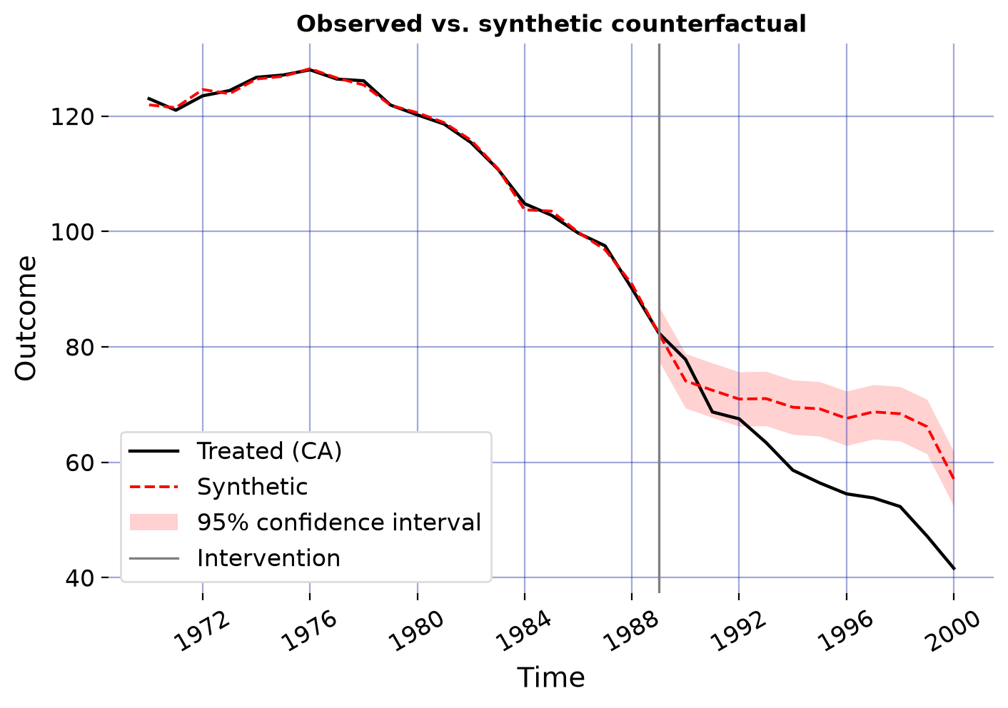
ca = result.effect_ci["CA"].assign(
    estimate=result.effects_panel["CA"], p_value=result.pointwise_p_values["CA"]
)
ca.round(2)| lower | upper | estimate | p_value | |
|---|---|---|---|---|
| 1989 | -4.64 | 4.80 | 0.08 | 1.00 |
| 1990 | -1.00 | 8.43 | 3.71 | 0.05 |
| 1991 | -8.48 | 0.96 | -3.76 | 0.05 |
| 1992 | -8.15 | 1.29 | -3.43 | 0.05 |
| 1993 | -12.33 | -2.90 | -7.61 | 0.00 |
| 1994 | -15.63 | -6.19 | -10.91 | 0.00 |
| 1995 | -17.55 | -8.12 | -12.83 | 0.00 |
| 1996 | -17.80 | -8.37 | -13.08 | 0.00 |
| 1997 | -19.63 | -10.19 | -14.91 | 0.00 |
| 1998 | -20.80 | -11.36 | -16.08 | 0.00 |
| 1999 | -23.68 | -14.24 | -18.96 | 0.00 |
| 2000 | -20.21 | -10.77 | -15.49 | 0.00 |
The effect is indistinguishable from zero in the first years. With 19 pre-treatment years the smallest attainable P value is \(1/19 \approx 0.053\), so the 1990–1992 estimates sit just short of the 5% threshold. From 1993 the effect is significant and keeps growing. The paper reads the slow start as consistent with addiction: consumption adjusts gradually to the tax.
result.plot(kind="spillover", display=False);findfont: Failed to find font weight medium, now using 400.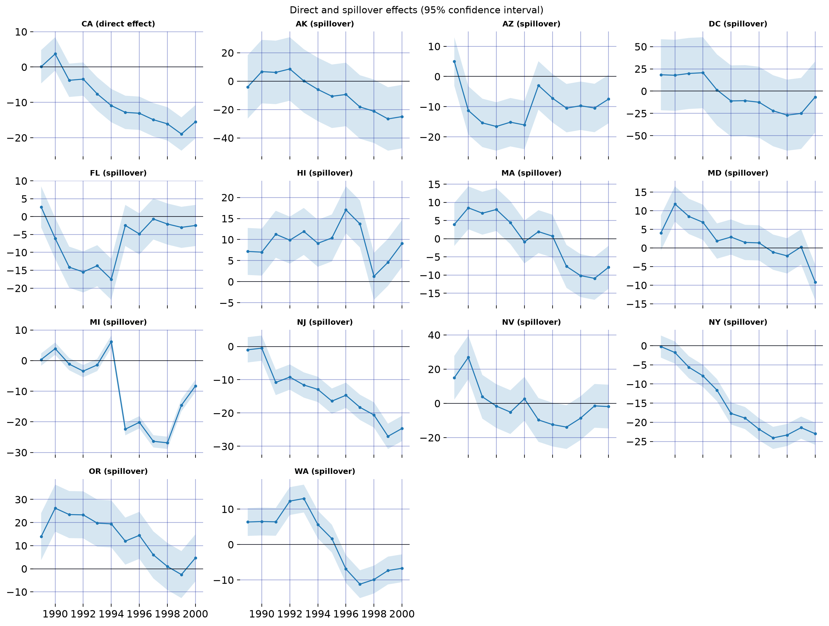
Nevada is the cleanest read: it had no tobacco law of its own in the 1990s, so its spillover is leakage rather than contamination.
nv = result.effect_ci["NV"].assign(
    estimate=result.effects_panel["NV"], p_value=result.pointwise_p_values["NV"]
)
nv.round(2).head(6)| lower | upper | estimate | p_value | |
|---|---|---|---|---|
| 1989 | 2.17 | 27.75 | 14.96 | 0.00 |
| 1990 | 14.07 | 39.65 | 26.86 | 0.00 |
| 1991 | -8.96 | 16.61 | 3.82 | 0.53 |
| 1992 | -14.40 | 11.17 | -1.62 | 0.79 |
| 1993 | -17.91 | 7.66 | -5.13 | 0.47 |
| 1994 | -10.12 | 15.45 | 2.67 | 0.58 |
Nevada’s consumption rises by roughly 15 and 27 packs per capita in the first two years, and the effect then fades. That is what cross-border buying predicts: smokers adapt, and later tax increases elsewhere narrow the price gap.
Is there any spillover at all? Test that every exposed state’s effect is zero, year by year:
import numpy as np
import pandas as pd

no_spillover = np.eye(len(result.unit_labels))[1:]  # every unit except California
pd.DataFrame(
    {
        t: {
            "statistic": result.test_hypothesis(no_spillover, period=t).statistic,
            "p_value": result.test_hypothesis(no_spillover, period=t).p_value,
            "reject": result.test_hypothesis(no_spillover, period=t).reject,
        }
        for t in result.effects_panel.index
    }
).T.round(3)| statistic | p_value | reject | |
|---|---|---|---|
| 1989 | 928.118746 | 0.263158 | False |
| 1990 | 2256.132741 | 0.0 | True |
| 1991 | 1871.335491 | 0.0 | True |
| 1992 | 2078.240119 | 0.0 | True |
| 1993 | 1440.352546 | 0.105263 | False |
| 1994 | 1745.839689 | 0.052632 | False |
| 1995 | 1725.34916 | 0.052632 | False |
| 1996 | 2120.186144 | 0.0 | True |
| 1997 | 3138.048987 | 0.0 | True |
| 1998 | 3248.095982 | 0.0 | True |
| 1999 | 3054.831627 | 0.0 | True |
| 2000 | 2232.312777 | 0.0 | True |
Everything above assumes the 13 exposed states are the only ones affected. The \(\kappa_A\) test checks that: the part of each post-treatment residual that the structure cannot explain should look like the pre-treatment residuals.
result.plot(kind="kappa", display=False);findfont: Failed to find font weight medium, now using 400.
findfont: Failed to find font weight medium, now using 400.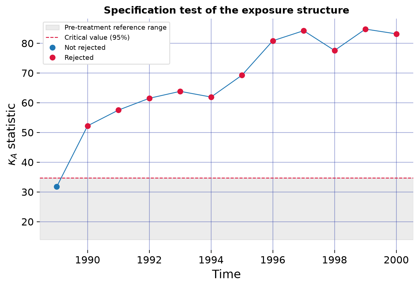
It rejects in every year after 1989. This is a real warning. Something moved after 1989 that the 13-state structure does not capture: national anti-smoking trends, other states’ policies, or spillovers on states assumed clean. Comparing candidate structures on the same fit shows that the paper’s choice still fits best among the obvious alternatives. A structure that nests another always fits at least as well, so this ranks the alternatives rather than validating the choice.
choice = result.select_structure_by_kappa(
    {
        "paper (13 states, per unit)": {"affected_units": list(panel.affected_units)},
        "13 states, one shared spillover": {
            "spillover_structure": "homogeneous",
            "affected_units": list(panel.affected_units),
        },
        "neighbours only": {"affected_units": ["AZ", "NV", "OR"]},
        "no spillovers": {"affected_units": []},
    }
)
choice.statistics.round(1).sort_values()
paper (13 states, per unit) 198.5
neighbours only 218.5
13 states, one shared spillover 222.3
no spillovers 224.3
Name: kappa_A (v3), dtype: float64If \(p\) of the states assumed clean received spillovers of at most \(\bar\alpha\), the bias of California’s effect is bounded linearly in \(\bar\alpha\) (Section 5.2.2 of the paper). The spillover-aware estimator’s bound grows far more slowly than that of a synthetic control built only from the clean states:
result.plot(kind="sensitivity", display=False);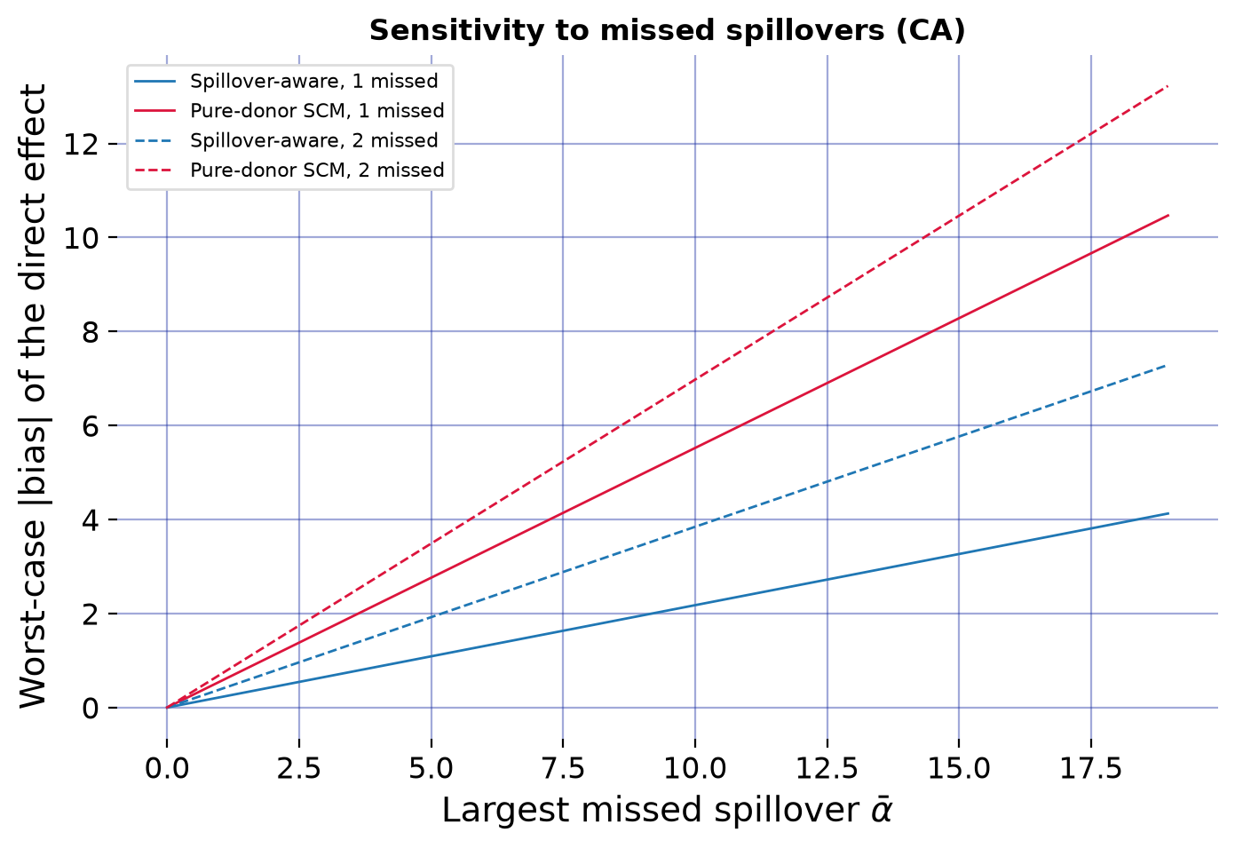
sens = result.cd.sensitivity
largest = result.effects_panel["CA"].max()
for p in (1, 2):
    c_sp, c_pd = sens.coefficients(p)
    print(
        f"p = {p}: a missed spillover of {largest / c_sp:.2f} packs could account for "
        f"California's largest estimate ({largest:.2f}); "
        f"{largest / c_pd:.2f} for the pure-donor SCM."
    )
p = 1: a missed spillover of 17.07 packs could account for California's largest estimate (3.71); 6.73 for the pure-donor SCM.
p = 2: a missed spillover of 9.66 packs could account for California's largest estimate (3.71); 5.33 for the pure-donor SCM.These are the break-even points the paper highlights in its Figure 3: 17.07 for one missed state and 9.66 for two.
The authors’ repository also drops the ten policy states that do not border California, leaving Arizona, Nevada and Oregon as the only exposed controls:
r41 = SCSPILL({**load_california_cd(41).config_kwargs(), "display_graphs": False}).fit()
pd.DataFrame(
    {"51 states": result.effects_panel["CA"], "41 states": r41.effects_panel["CA"]}
).round(2).T| 1989 | 1990 | 1991 | 1992 | 1993 | 1994 | 1995 | 1996 | 1997 | 1998 | 1999 | 2000 | |
|---|---|---|---|---|---|---|---|---|---|---|---|---|
| 51 states | 0.08 | 3.71 | -3.76 | -3.43 | -7.61 | -10.91 | -12.83 | -13.08 | -14.91 | -16.08 | -18.96 | -15.49 |
| 41 states | -0.97 | 4.18 | -4.83 | -4.52 | -8.55 | -8.94 | -13.96 | -14.16 | -15.94 | -15.97 | -20.24 | -16.82 |
cd and sar, side by sideThe Get started page fits sar to the classic panel. The two analyses differ in more than the model, so read the comparison with care:
cd (this page) |
sar (Get started) |
|
|---|---|---|
| Panel | Cao & Dowd: 50 states + DC | Abadie et al.: 39 states (the 12 policy states dropped) |
| Outcome | per-capita consumption (cigs) |
per-capita sales (cigsale) |
| Treated from | 1989 | 1988 |
| Spillover assumption | free effects on 13 named states | one intensity \(\rho\) through rook contiguity |
| Inference | P tests from the pre-treatment residuals | Bayesian posterior |
from scspill.data import load_california

sar = SCSPILL(
    {**load_california().config_kwargs(), "m_iter": 4000, "burn": 2000, "seed": 42,
     "display_graphs": False}
).fit()
print(f"sar: ATT {sar.att:.1f} (95% CrI [{sar.att_ci[0]:.1f}, {sar.att_ci[1]:.1f}]), "
      f"rho {sar.rho_hat:.2f}")
print(f"cd:  ATT {result.att:.1f} (no interval for the average)")
sar: ATT -17.1 (95% CrI [-23.0, -11.0]), rho 0.37
cd: ATT -9.4 (no interval for the average)import matplotlib.pyplot as plt
fig, ax = plt.subplots(figsize=(8, 4.5))
years = result.effects_panel.index
ax.fill_between(years, result.effect_ci["CA"]["lower"], result.effect_ci["CA"]["upper"],
alpha=0.2, color="#1f77b4")
ax.plot(years, result.effects_panel["CA"], "o-", color="#1f77b4", label="cd (51 units, from 1989)")
t0 = sar.inputs.T0
sar_years = sar.inputs.time_labels[t0:]
gap = sar.inputs.Y0[t0:] - sar.effects_detail.cf_mean[t0:]
ax.fill_between(sar_years, sar.inputs.Y0[t0:] - sar.effects_detail.cf_upper[t0:],
sar.inputs.Y0[t0:] - sar.effects_detail.cf_lower[t0:], alpha=0.2, color="crimson")
ax.plot(sar_years, gap, "s-", color="crimson", label="sar (39 states, from 1988)")
ax.axhline(0, color="black", linewidth=0.8)
ax.set_xlabel("Year")
ax.set_ylabel("Effect on California (packs per capita)")
ax.legend();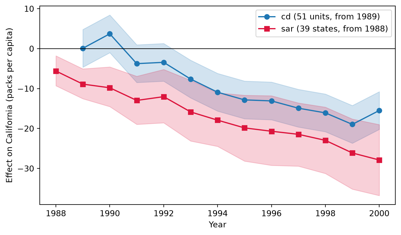
The models agree that the program cut consumption and that the cut grew over the decade. They disagree about Nevada:
pd.DataFrame(
    {
        "cd: spillover on NV": result.effects_panel["NV"].loc[1989:1992],
        "sar: spillover on Nevada": sar.spillover_panel["Nevada"].loc[1989:1992],
    }
).round(2)| cd: spillover on NV | sar: spillover on Nevada | |
|---|---|---|
| 1989 | 14.96 | -3.45 |
| 1990 | 26.86 | -3.81 |
| 1991 | 3.82 | -5.04 |
| 1992 | -1.62 | -4.67 |
cd leaves the size and sign of each spillover free, and finds Nevada’s consumption rising: leakage. sar routes every spillover through one intensity \(\rho\) applied to California’s own outcome. Its estimate here is positive, so a fall in California is passed on as a fall in its neighbours. A negative \(\rho\) could express leakage, but the one intensity governs every channel at once, and in this sample the data put it above zero. Neither answer is “the” answer. The two models make different assumptions, so running both shows how much the conclusion depends on the spillover assumption.
cd intervals come from 19 pre-treatment residuals. That limits the smallest attainable P value to \(1/19\), and it makes the leave-one-period-out references (reference_mode="leave_one_period_out") noticeably wider.cd model in practice takes the disagreements further. It fits both models on all three samples to separate model from sample, and it diagnoses the structure test’s rejection.