flowchart TB
    subgraph "California"
        CA_pre["Pre (1984–88) mean<br/>= 99.0"] --> CA_d["Δ California =<br/>72.0 − 99.0 = −27.0"]
        CA_post["Post (1989–93) mean<br/>= 72.0"] --> CA_d
    end
    subgraph "Nevada (control)"
        NV_pre["Pre (1984–88) mean<br/>= 143.1"] --> NV_d["Δ Nevada =<br/>121.8 − 143.1 = −21.3"]
        NV_post["Post (1989–93) mean<br/>= 121.8"] --> NV_d
    end
    CA_d --> DD["DiD ATT =<br/>(−27.0) − (−21.3) = −5.7"]
    NV_d --> DD

    style CA_pre fill:#d97757,stroke:#cbd5e0,color:#fff
    style CA_post fill:#d97757,stroke:#cbd5e0,color:#fff
    style NV_pre fill:#6a9bcc,stroke:#cbd5e0,color:#fff
    style NV_post fill:#6a9bcc,stroke:#cbd5e0,color:#fff
    style DD fill:#00d4c8,stroke:#cbd5e0,color:#141413
3 Basic Differences-in-Differences
3.1 Learning objectives
- Construct the 2×2 DiD grid (treated vs. one control, pre vs. post) and recover the ATT as the difference of differences. This is the simplest causal contrast in the book and the conceptual anchor every later DiD generalization builds on.
- Estimate the 2×2 DiD as a single OLS interaction (
cigsale ~ state * prepost) and read the ATT off the interaction coefficient. The regression form is what scales to covariates and time-varying treatments in later chapters. - Test the parallel-trends assumption formally by fitting
cigsale ~ state * yearon the pre-period and checking whether the slope-difference interaction is zero. A reader who only “eyeballs” parallel trends has no defence against a referee who fits the regression. - Compute HAC-robust standard errors with
sandwich::vcovHACand explain why cluster-robust inference collapses at \(G = 2\). This is the practical inference fix every 2-unit DiD needs, and naming the collapse keeps the reader from defaulting to a brokencluster = statecall.
3.2 The DiD idea
Chapter 2 showed that any within-unit method — growth curve, ARIMA — is fragile because the counterfactual is identified only by an assumption the data cannot verify. Difference-in-Differences borrows strength from outside California by adding one control unit, replacing an extrapolation assumption with a comparability assumption.
DiD picks one control state — Nevada, for this chapter — and treats its pre-to-post change as the counterfactual change California would have experienced absent the policy. Subtract Nevada’s change from California’s change. Whatever is left over is “what the policy did”. The canonical applied example is Card & Krueger (1994), who compared fast-food employment in New Jersey and Pennsylvania around New Jersey’s 1992 minimum-wage hike.
The identifying assumption is parallel trends: California and Nevada would have moved on parallel paths without the policy. Differences in levels are fine; differences in trends are not. The estimand is a proper Average Treatment effect on the Treated (ATT) for California.
3.3 The change-of-changes identity
The formal DiD identity is
\[\widehat{\tau}_{\text{DiD}} \,=\, \big(\bar{Y}_{\text{CA, post}} - \bar{Y}_{\text{CA, pre}}\big) - \big(\bar{Y}_{\text{NV, post}} - \bar{Y}_{\text{NV, pre}}\big).\]
In the chapter 1 notation, this is the imputation \(\widehat{Y_{1t}(0)} = \overline{Y}_{1,\text{pre}} + (\overline{Y}_{0,\text{post}} - \overline{Y}_{0,\text{pre}})\) — California’s pre-period mean plus Nevada’s pre-to-post change.
The matching population regression is
\[Y_{it} = \alpha + \beta_1 \, \mathrm{Post}_t + \beta_2 \, \mathrm{Treat}_i + \tau \, (\mathrm{Post}_t \times \mathrm{Treat}_i) + u_{it},\]
where \(\mathrm{Treat}_i = 1\) for California and \(0\) for Nevada, and \(\mathrm{Post}_t = 1\) for \(t \ge 1989\). The OLS estimator \(\widehat{\tau}\) of the interaction coefficient is the DiD ATT — algebraically identical to the change-of-changes identity above, but in a form that gives us a standard error. We refer to this estimator as \(\widehat{\tau}_{\text{DiD}}\) throughout.
The four ingredients of the DiD calculation are easier to see as a 2×2 grid. Each cell holds a group mean; the two within-state changes are the row differences; the DiD estimate is the difference of those differences.
3.4 Setup and data
Packages. tidyverse covers wrangling and plotting. sandwich and lmtest supply the heteroskedasticity-and-autocorrelation-consistent (HAC) standard errors used in the regression below. Inference on a 2×2 panel is genuinely awkward — see the “Fit and HAC inference” section for an honest discussion of why HAC is a compromise rather than a textbook fix (Bertrand et al., 2004). The R/table_helpers.R helper provides ms_pretty(), the modelsummary wrapper that styles the fitted regression table.
Code: Load packages, source table helpers, and set the transparent ggplot theme.
library(tidyverse)
library(sandwich)
library(lmtest)
source("R/table_helpers.R")

# set.seed not strictly needed here — OLS and means are deterministic —
# but kept for consistency with the rest of the book.
set.seed(42)

knitr::opts_chunk$set(dev.args = list(bg = "transparent"))

theme_set(
  theme_minimal(base_size = 12) +
    theme(
      plot.background  = element_rect(fill = "transparent", color = NA),
      panel.background = element_rect(fill = "transparent", color = NA),
      panel.grid.major = element_line(color = "#94a3b8", linewidth = 0.25),
      panel.grid.minor = element_line(color = "#94a3b8", linewidth = 0.15),
      text             = element_text(color = "#94a3b8"),
      axis.text        = element_text(color = "#94a3b8")
    )
)
Dataset. DiD trades the comparison-unit problem for a smaller, sharper subset of the panel. From the full 39-state × 31-year dataset we keep only California and Nevada and only the 1984–1993 window — five pre-period years (1984–1988) and five post-period years (1989–1993). Nevada is the hand-picked control, chosen as a geographically and demographically adjacent state. (Reno and Las Vegas both sit inside California’s media market and share its retail-price corridor; Nevada was also one of the donor states with non-zero weight in Abadie, Diamond & Hainmueller’s synthetic California — see chapter 4.) The state factor is releveled with Nevada as the reference so that the stateCalifornia and stateCalifornia:prepostPost coefficients land on California’s main effect and extra change relative to Nevada — the DiD coefficient is the latter.
Code: Load Prop 99 data and subset to California and Nevada in 1984-1993 with a Pre/Post factor.
prop99 <- read_rds("data/proposition99.rds") |> as_tibble()

# Keep only California and Nevada in the 1984-1993 window and add the
# Pre/Post factor. Make Nevada the reference level so that the
# stateCalifornia interaction lands on California's extra change.
prop99_did <- prop99 |>
  filter(state %in% c("California", "Nevada"),
         year > 1983, year < 1994) |>
  mutate(prepost = factor(year > 1988, labels = c("Pre", "Post")),
         state   = factor(state, levels = c("Nevada", "California")))
The resulting prop99_did tibble has 20 rows (2 states × 10 years) and four columns: state, year, cigsale, and prepost. Those are the only inputs the DiD regression needs.
3.5 Fit and HAC inference
The model. The two-way interacted OLS cigsale ~ state * prepost is the regression form of the 2×2 grid above — the arithmetic in the grid is literally what this regression computes. The four estimated coefficients map one-to-one onto the grid cells: the intercept is the Nevada–Pre cell, stateCalifornia shifts up or down to land on the California–Pre cell, prepostPost shifts to the Nevada–Post cell, and the interaction stateCalifornia:prepostPost is exactly the DiD ATT \(\widehat{\tau}_{\text{DiD}}\) — the extra California change beyond what happened to Nevada over the same window.
Standard errors on a 2×2 panel are tricky. Textbook OLS SEs assume i.i.d. errors, which fails here because within-state residuals are serially correlated over the ten-year window. The standard fix — clustering by state (Bertrand et al., 2004) — is degenerate with only two clusters: the cluster-robust variance estimator’s asymptotic theory requires the number of clusters \(G\) to grow, and at \(G = 2\) it collapses to a single 2×2 outer product. Software will compute a number; one cannot interpret it. We report HAC-robust SEs via sandwich::vcovHAC as a transparent compromise: they correct for within-unit autocorrelation by treating the stacked panel as a long time series, but they ignore the cross-state row boundary in the stacked design. The qualitative reading — that the DiD point estimate is statistically indistinguishable from zero — survives every reasonable choice; readers should treat the \(p\)-value as a rough heuristic, not a textbook test.
Code: Fit the two-way interacted DiD regression and report HAC-robust standard errors.
# Two-way interacted regression: state main effect + Pre/Post main effect
# + (state x Pre/Post) interaction. The interaction is the DiD estimate.
fit_did <- lm(cigsale ~ state * prepost, data = prop99_did)

# HAC-robust standard errors for the four coefficients.
ms_pretty(list("Two-way interacted OLS, HAC SEs" = fit_did),
          vcov     = sandwich::vcovHAC,
          coef_map = c("(Intercept)"                  = "Nevada · Pre (baseline)",
                       "stateCalifornia"              = "California main",
                       "prepostPost"                  = "Post main",
                       "stateCalifornia:prepostPost"  = "DiD interaction"),
notes = "Standard errors HAC-robust via sandwich::vcovHAC.")| Two-way interacted OLS, HAC SEs | |
|---|---|
| Nevada · Pre (baseline) | 143.100*** |
| (1.092) | |
| California main | -44.120*** |
| (3.880) | |
| Post main | -21.340* |
| (7.687) | |
| DiD interaction | -5.680 |
| (5.393) | |
| Num.Obs. | 20 |
| R2 | 0.914 |
| Std.Errors | Custom |
| + p < 0.1, * p < 0.05, ** p < 0.01, *** p < 0.001 | |
| Standard errors HAC-robust via sandwich::vcovHAC. | |
Reading the output. The interaction coefficient \(\widehat{\tau}_{\text{DiD}}\) (R name: stateCalifornia:prepostPost) is -5.68 packs (HAC SE \(\approx\) 5.39, \(p \approx\) 0.31). That is dramatically smaller than California’s own within-state pre-to-post change of -27.0 packs over this 1984–1993 window, and statistically indistinguishable from zero. Why? Because the prepostPost main effect — Nevada’s own pre-to-post change — is also large at -21.34 packs. When DiD subtracts that Nevada change from California’s change, almost all of California’s drop is absorbed.
3.6 Visual diagnostic
What to look for. DiD rests entirely on the parallel-trends assumption: that California and Nevada would have moved in lockstep absent the policy. The data themselves cannot prove this counterfactual, but we can at least inspect the pre-period by plotting both states on the same axes over the full 1970–2000 window. Three features matter visually: (1) do the two pre-1989 lines move roughly in parallel? (2) does Nevada also bend downward after 1989, and if so, by how much? (3) is the post-1989 gap between California and Nevada much bigger than the pre-period gap? If Nevada is itself trending down post-1989, the DiD contrast collapses — the Nevada change subtracts away most of California’s drop.
Code: Plot California vs Nevada cigarette sales over 1970-2000 with a 1988.5 policy cutoff.
two_states <- prop99 |>
  filter(state %in% c("California", "Nevada"))

ggplot(two_states, aes(x = year, y = cigsale, color = state)) +
  geom_line(linewidth = 1.1) +
  geom_vline(xintercept = 1988.5, color = "#94a3b8",
             linetype = "dashed", linewidth = 0.7) +
  scale_color_manual(values = c("California" = "#d97757",
                                "Nevada"     = "#6a9bcc")) +
  labs(x = "Year", y = "Cigarette sales (packs per capita)",
       color = NULL)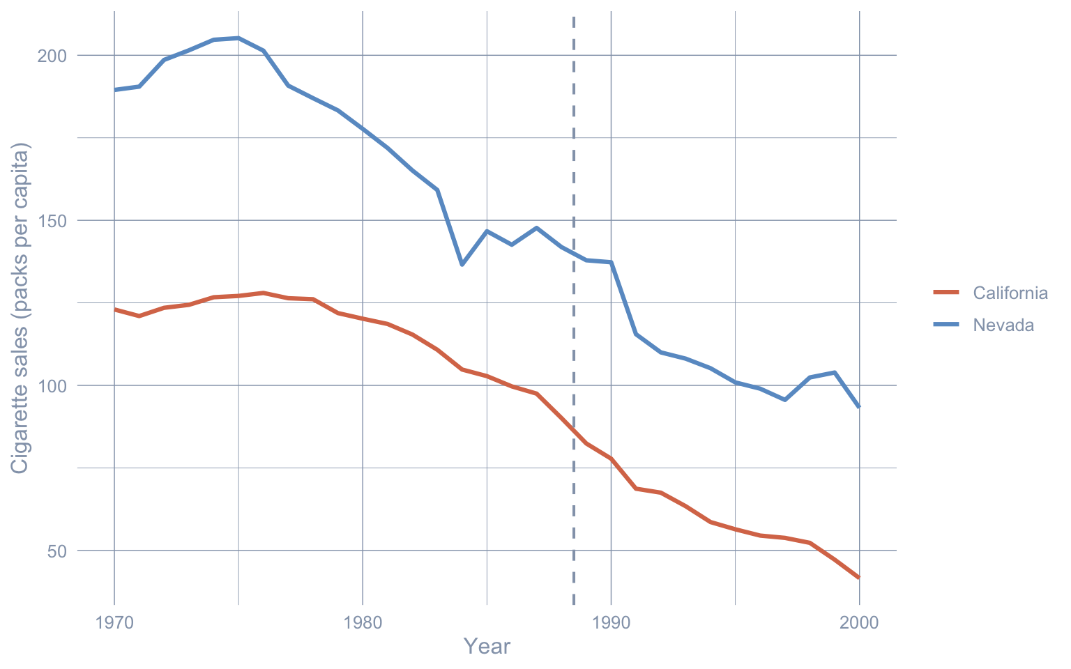
Formal pre-trends test. The visual is suggestive, but parallel trends is a claim about slopes in the pre-period, and we can test it directly. Fit cigsale ~ state * year on the 1984–1988 pre-window: if parallel trends holds, the stateCalifornia:year interaction — the slope difference between the two states’ pre-period paths — should be statistically indistinguishable from zero.
Code: Test parallel pre-trends by regressing cigsale on state-by-year over 1984-1988.
pre_window <- prop99_did |> filter(prepost == "Pre")
fit_pre <- lm(cigsale ~ state * year, data = pre_window)

ms_pretty(list("Pre-trend slope test (1984-1988)" = fit_pre),
          vcov     = sandwich::vcovHAC,
          coef_map = c("(Intercept)"          = "Nevada baseline",
                       "stateCalifornia"      = "California level shift",
                       "year"                 = "Nevada slope",
                       "stateCalifornia:year" = "Slope difference (CA - NV)"),
notes = "If parallel trends held, the slope difference should be ~0.")| Pre-trend slope test (1984-1988) | |
|---|---|
| Nevada baseline | -2160.655 |
| (3006.082) | |
| California level shift | 9151.058* |
| (3052.496) | |
| Nevada slope | 1.160 |
| (1.514) | |
| Slope difference (CA - NV) | -4.630* |
| (1.537) | |
| Num.Obs. | 10 |
| R2 | 0.985 |
| Std.Errors | Custom |
| + p < 0.1, * p < 0.05, ** p < 0.01, *** p < 0.001 | |
| If parallel trends held, the slope difference should be ~0. | |
The slope-difference estimate is -4.63 packs per year with HAC \(p \approx\) 0.024. Even before Proposition 99, California was declining roughly 4.6 packs/year faster than Nevada — i.e. the two series were already diverging in the direction the policy would later push, so the parallel trends assumption is rejected by the pre-period data themselves. This is load-bearing: it turns the chapter’s diagnosis from “Nevada has its own decline (visible in the plot)” into “California was already separating from Nevada (testable, rejected)”. The test is a falsification check: failing it disqualifies the design, but passing it does not prove parallel trends in the post-period — the missing-data nature of the counterfactual is untestable by construction.
This is the textbook DiD pitfall. A single control unit that itself is shifting in the same direction makes the contrast collapse. Nevada is geographically and culturally adjacent to California. It inherits many of the same secular forces: rising health awareness, federal tobacco settlements, retail-price spillovers. So it is a poor “what would California have done?” control.
Common pitfall. Picking the one “most similar” control by hand. If your single control is subject to the same secular forces as the treated unit — geographic neighbours, policy spillovers, regional macro shocks — the contrast collapses and DiD silently reports zero.
A second pitfall. Clustering standard errors by state on a two-state panel. The cluster-robust variance estimator (Bertrand et al., 2004) requires the number of clusters to grow; at \(G = 2\) it collapses to a single 2×2 outer product and is uninterpretable. Software will compute a number; do not trust it. With only two units, accept that classical inference on the DiD coefficient is unavailable and let the point estimate carry the argument.
A third pitfall. Treating Nevada as causally exogenous. Nevada borders California on a 600-km stretch, sits inside California’s TV-advertising and retail-price corridor, and inherits its anti-smoking media spillovers. The “control” is not policy-untreated in the deep sense — only in the narrow sense of not having passed Proposition 99 itself.
Recap. DiD against Nevada returns \(\widehat{\tau}_{\text{DiD}} \approx\) -5.68 packs and we cannot reject zero. The lesson is not that DiD is broken — it is that DiD with a single similar control unit is fragile, and the pre-trends test makes that fragility formal rather than merely visual. Synthetic Control (chapter 4) is the principled response: instead of one neighbour, blend many Nevadas into a weighted synthetic California — the optimisation picks the weights so the analyst no longer has to hand-pick the control.
3.7 Key takeaways
Methods:
- Difference-in-Differences (DiD) is a 2×2 contrast that estimates the Average Treatment effect on the Treated (ATT) as \(\widehat{\tau}_{\text{DiD}} = (\bar Y_{\text{CA,post}} - \bar Y_{\text{CA,pre}}) - (\bar Y_{\text{NV,post}} - \bar Y_{\text{NV,pre}})\) — California’s pre-to-post change minus Nevada’s, with the control’s change imputing California’s missing \(Y_{1t}(0)\).
- The two-way interacted regression
cigsale ~ state * prepostis the regression form of that 2×2 grid; with one treated unit and one control, thestate:prepostinteraction is algebraically identical to the change-of-changes ATT and is equivalent to the unit-and-period two-way fixed-effects specification on this balanced panel. - Identification rests on parallel trends — California and Nevada would have evolved on parallel paths absent Proposition 99. Differences in levels between the two states are absorbed by the unit fixed effect; only differences in trends bias the DiD estimand.
Lessons:
- Adding even one outside comparison unit dramatically shrinks the estimated effect. California’s within-state pre-to-post change of -27.0 packs over the 1984–1993 window collapses to \(\widehat{\tau}_{\text{DiD}} \approx\) -5.68 packs once Nevada’s own -21.3-pack pre-to-post change is subtracted off, and the resulting ATT is statistically indistinguishable from zero.
- Inspect parallel trends both visually and formally. Regressing
cigsale ~ state * yearon the 1984–1988 pre-window yields a slope difference of -4.63 packs/year (\(p \approx\) 0.024): California was already declining faster than Nevada before the policy, so parallel trends is rejected by the pre-period data themselves. - A failed pre-trends test reframes the chapter’s headline. The shrinkage is not just “Nevada has its own decline” but “California was already separating from Nevada in the policy’s direction” — meaning DiD against Nevada absorbs genuine treatment signal into a non-parallel counterfactual.
Caveats:
- Hand-picking a single “most similar” control is the textbook DiD pitfall. Geographic and cultural neighbours like Nevada inherit the same secular forces as the treated unit — rising health awareness, federal tobacco settlements, California-media spillovers — so the contrast can silently collapse to zero. Synthetic control (chapter 4) is the principled response: blend many donors into a weighted synthetic California rather than choose one neighbour by hand.
- Inference on a 2×2 panel is genuinely awkward. Clustering by state is degenerate at \(G = 2\) clusters; HAC-robust SEs via
sandwich::vcovHACare a transparent compromise that ignore the cross-state row boundary, so the reported \(p\)-value should be read as a rough heuristic rather than a textbook test. - This single-shock, single-treated-unit DiD is a deliberately simple base case. With many units adopting at staggered dates, two-way fixed-effects DiD can be biased by treatment-effect heterogeneity; chapter 8 revisits the staggered-adoption setting with the Callaway–Sant’Anna group-time ATT and Rambachan–Roth honest-DiD sensitivity bounds.
3.8 Further reading
This chapter is the canonical 2×2 / single-shock DiD: one treated unit (California), one control unit (Nevada), one pre-period, one post-period. Chapter 8 (Part II) revisits DiD in the staggered-adoption setting — many treated units that switch at different dates — using the Callaway–Sant’Anna group-time ATT estimator, the Sun–Abraham interaction-weighted estimator, and the Rambachan–Roth honest-DiD sensitivity bounds on a minimum-wage county panel. The two chapters together cover the modern DiD toolkit.
- Card & Krueger (1994) — applied example — the textbook 2×2 DiD on New Jersey vs Pennsylvania minimum wage and fast-food employment; the historical template for the design in this chapter.
- Bertrand et al. (2004) — seminal warning — DiD standard errors are biased toward zero under residual autocorrelation, and the cluster-robust fix requires the number of clusters to grow; the reason this chapter’s inference choice is non-trivial at \(G = 2\).
- Bernal et al. (2017) — tutorial — practitioner reference for parallel-trends visual diagnostics in a public-health setting.
- Roth et al. (2023) — review — a synthesis of the recent DiD econometrics literature, useful for orienting between the 2×2 case here and the staggered-adoption machinery of chapter 8.
- Callaway (2022) — handbook chapter — a longer-form treatment of DiD for policy evaluation that motivates the move from the 2×2 design to group-time ATTs.
3.9 Exercises
These exercises drill on the four ideas the chapter introduces: the 2×2 grid is literally what the OLS interaction computes; the choice of control state is a load-bearing analyst decision; the parallel-trends assumption is testable on the pre-window; and HAC inference is a compromise, not a fix, on a \(G = 2\) panel. They reuse prop99 and prop99_did from the setup chunks; nothing needs to be re-loaded.
3.9.1 Exercise 1: Recover the 2×2 grid by hand
Compute the four cell means in the DiD grid (California × {Pre, Post} and Nevada × {Pre, Post}) directly with group_by() / summarize(). Take the difference of differences and verify it matches the stateCalifornia:prepostPost interaction coefficient from the chapter’s fit_did regression.
TipSolution
Code
grid <- prop99_did |>
  group_by(state, prepost) |>
  summarize(mean_cigsale = mean(cigsale), .groups = "drop") |>
  pivot_wider(names_from = prepost, values_from = mean_cigsale) |>
  mutate(change = Post - Pre)

did_by_hand <- grid$change[grid$state == "California"] -
               grid$change[grid$state == "Nevada"]

list(grid       = grid,
     did_hand   = did_by_hand,
     did_coef   = coef(fit_did)[["stateCalifornia:prepostPost"]])
$grid
# A tibble: 2 × 4
state Pre Post change
<fct> <dbl> <dbl> <dbl>
1 Nevada 143. 122. -21.3
2 California 99.0 72.0 -27.0
$did_hand
[1] -5.679999
$did_coef
[1] -5.679999The hand-computed difference-of-differences (\(\approx -5.7\)) is identical to the fit_did interaction coefficient. The interaction in cigsale ~ state * prepost does no statistical magic — it is the arithmetic of the 2×2 grid expressed in matrix form, with the bonus that the regression also gives us a standard error.
3.9.2 Exercise 2: Swap Nevada for Montana
Refit the DiD with Montana as the single control state in place of Nevada (1984–1993 window). Report the new DiD ATT and HAC SE. Does the qualitative reading from the chapter — “statistically indistinguishable from zero” — survive a different control choice?
TipSolution
Code
prop99_did_mt <- prop99 |>
  filter(state %in% c("California", "Montana"),
         year > 1983, year < 1994) |>
  mutate(prepost = factor(year > 1988, labels = c("Pre", "Post")),
         state   = factor(state, levels = c("Montana", "California")))

fit_did_mt <- lm(cigsale ~ state * prepost, data = prop99_did_mt)

ms_pretty(list("California vs Montana DiD (1984-1993)" = fit_did_mt),
          vcov     = sandwich::vcovHAC,
          coef_map = c("(Intercept)"                  = "Montana · Pre",
                       "stateCalifornia"              = "California main",
                       "prepostPost"                  = "Post main",
"stateCalifornia:prepostPost" = "DiD interaction"))| California vs Montana DiD (1984-1993) | |
|---|---|
| Montana · Pre | 98.060*** |
| (4.019) | |
| California main | 0.920 |
| (3.311) | |
| Post main | -12.780** |
| (4.090) | |
| DiD interaction | -14.240** |
| (4.232) | |
| Num.Obs. | 20 |
| R2 | 0.771 |
| Std.Errors | Custom |
| + p < 0.1, * p < 0.05, ** p < 0.01, *** p < 0.001 | |
The Montana-DiD ATT is markedly more negative than the Nevada-DiD ATT, because Montana’s own post-period decline was smaller than Nevada’s — Montana subtracts less of California’s drop. The point estimate is now visually larger but the HAC SE on a 2×2 panel is still wide; the qualitative reading depends on the analyst’s control choice. This is the chapter’s “first pitfall” made operational: with \(N = 2\) states, the entire estimate hangs on one human decision.
3.9.3 Exercise 3: Long-window parallel-trends test
The chapter’s pre-trend test uses only 1984–1988 (5 years). Re-run the slope-difference test on a wider 1980–1988 window (9 years) and compare the \(p\)-value. Does a longer pre-window strengthen or weaken the parallel-trends rejection?
TipSolution
Code
long_pre <- prop99 |>
  filter(state %in% c("California", "Nevada"),
         year >= 1980, year <= 1988) |>
  mutate(state = factor(state, levels = c("Nevada", "California")))

fit_pre_long <- lm(cigsale ~ state * year, data = long_pre)

ms_pretty(list("Pre-trend test (1980-1988)" = fit_pre_long),
          vcov     = sandwich::vcovHAC,
          coef_map = c("(Intercept)"          = "Nevada baseline",
                       "stateCalifornia"      = "California level shift",
                       "year"                 = "Nevada slope",
"stateCalifornia:year" = "Slope difference (CA - NV)"))| Pre-trend test (1980-1988) | |
|---|---|
| Nevada baseline | 9191.498*** |
| (1679.346) | |
| California level shift | -1707.669 |
| (1893.881) | |
| Nevada slope | -4.555*** |
| (0.847) | |
| Slope difference (CA - NV) | 0.837 |
| (0.955) | |
| Num.Obs. | 18 |
| R2 | 0.963 |
| Std.Errors | Custom |
| + p < 0.1, * p < 0.05, ** p < 0.01, *** p < 0.001 | |
With nine years of pre-period data the slope-difference estimate stays negative and the standard error shrinks; the parallel-trends rejection therefore strengthens. The chapter’s choice of 1984–1988 was not hiding a passable pre-trend — California and Nevada were already diverging at least as early as 1980. A reader who only saw the 1984–1988 test might wonder whether the rejection was a short-window artifact; this longer window rules that out.
3.9.4 Exercise 4: HAC vs classical OLS standard errors
Refit the DiD and compare three standard-error choices for the DiD interaction: classical OLS, HAC via sandwich::vcovHAC, and HC1 (“White”) via sandwich::vcovHC. Which is biggest, which is smallest, and why does the textbook fix (cluster by state) not appear in the comparison?
TipSolution
Code
ms_pretty(list("Classical OLS"        = fit_did,
               "HC1 (White)"          = fit_did,
               "HAC (Andrews/vcovHAC)" = fit_did),
          vcov     = list(NULL,
                          sandwich::vcovHC,
                          sandwich::vcovHAC),
coef_map = c("stateCalifornia:prepostPost" = "DiD interaction"))| Classical OLS | HC1 (White) | HAC (Andrews/vcovHAC) | |
|---|---|---|---|
| DiD interaction | -5.680 | -5.680 | -5.680 |
| (8.127) | (9.087) | (5.393) | |
| Num.Obs. | 20 | 20 | 20 |
| R2 | 0.914 | 0.914 | 0.914 |
| Std.Errors | Custom | Custom | |
| + p < 0.1, * p < 0.05, ** p < 0.01, *** p < 0.001 | |||
Classical OLS underestimates the SE because it assumes within-state residuals are independent; HC1 is similar — it corrects for heteroskedasticity but not autocorrelation. HAC is the largest because it explicitly inflates the SE for serial correlation across the ten-year window. Cluster-by-state is not in the comparison because \(G = 2\): the cluster-robust variance estimator’s asymptotic theory needs the number of clusters to grow, and at two clusters it collapses to a single 2×2 outer product. Software will produce a number; the number has no statistical meaning. With only two units, accept the HAC compromise and let the point estimate carry the argument — or move to synthetic control (ch. 4), where placebo-based inference replaces classical SEs.
3.9.5 Exercise 5 (stretch): Pool three control states into a TWFE-like DiD
Extend the 2×2 panel to three control states — Nevada, Montana, and Colorado — keeping California treated and the 1984–1993 window. Fit a two-way-fixed-effects-style regression of cigsale on state and period dummies plus a treat_post indicator that equals one only for California in 1989–1993, and compare the treat_post coefficient (the DiD ATT) to the Nevada-only and Montana-only versions above.
TipSolution
Code
pool4 <- prop99 |>
  filter(state %in% c("California", "Nevada", "Montana", "Colorado"),
         year > 1983, year < 1994) |>
  mutate(prepost    = factor(year > 1988, labels = c("Pre", "Post")),
         treat_post = as.integer(state == "California" & year > 1988))

fit_pool <- lm(cigsale ~ state + prepost + treat_post, data = pool4)

ms_pretty(list("Pooled 3-control DiD" = fit_pool),
          vcov     = sandwich::vcovHAC,
coef_map = c("treat_post" = "DiD interaction"))| Pooled 3-control DiD | |
|---|---|
| DiD interaction | -9.267*** |
| (1.829) | |
| Num.Obs. | 40 |
| R2 | 0.890 |
| Std.Errors | Custom |
| + p < 0.1, * p < 0.05, ** p < 0.01, *** p < 0.001 | |
The pooled-controls DiD lands between the Nevada-only and Montana-only estimates from earlier exercises — pooling averages the implicit weight given to each control. The SE shrinks because we now have \(G = 4\) effective units and \(4 \times 10 = 40\) observations rather than 20. This is conceptually the bridge to synthetic control (ch. 4), which generalises the uniform averaging across donors here to an optimised weighted blend whose weights are pinned down by the pre-period match.