---
title: "Staggered Differences-in-Differences"
---
## Learning objectives
1. Estimate group-time average treatment effects with `did::att_gt()` on a staggered-adoption panel. This is the workhorse of modern DiD — the estimator that replaced two-way fixed effects after the negative-weight critique.
2. Aggregate group-time effects into event-study dynamics with `aggte(type = "dynamic")`. The aggregation step is what gives the reader a single defensible event-study plot without the contamination problems of a TWFE event study.
3. Condition on covariates using regression, IPW, and doubly-robust estimators, and default to the doubly-robust choice. Doubly-robust estimation is consistent if *either* the outcome model or the propensity-score model is correctly specified, which is why it is the safe default — knowing all three lets the reader defend that choice against a referee.
4. Run Rambachan-Roth relative-magnitudes sensitivity analysis with `HonestDiD` and report the smallest pre-trend violation that would overturn the post-treatment conclusion. This converts an unverifiable parallel-trends assumption into a falsifiable claim about how robust the headline result is.
::: {.callout-note appearance="simple"}
**Part II begins here.** Chapters 2–9 held the dataset fixed
(Proposition 99) and varied the estimator. From this chapter forward
we switch datasets too: a 1,745-county minimum-wage panel with
*staggered* adoption replaces California's single-shock setting, and
the toolkit shifts to estimators built for that structure.
:::
## When TWFE breaks under staggered adoption
Chapter 3 ran a textbook 2×2 DiD on Proposition 99: California
treated in 1989, Nevada as the single hand-picked control. That
design squeezed the entire causal contrast into one interaction
coefficient — $\widehat{\tau}_{\text{DiD}} \approx -5.7$ packs per
capita, statistically indistinguishable from zero. The diagnosis
there was twofold: Nevada inherits California's secular forces (so
its own post-1988 decline soaks up most of the policy signal), *and*
parallel trends was rejected on the pre-window itself.
That design has a deeper structural limit. Real policy data rarely
has just one treated unit and one clean control unit, both switching
at the same instant. States and counties **adopt at different times**
— some in 2004, others in 2006, still others never. The natural
extension of the chapter-3 regression to that setting is the
*two-way fixed-effects (TWFE)* specification:
$$Y_{it} = \alpha_i + \gamma_t + \beta \cdot \text{post}_{it} + \varepsilon_{it}.$$
For two decades this was the default. We now know it is biased in the
presence of staggered adoption: already-treated units silently act as
*controls* for later-treated units, contaminating the contrast. The
@goodmanbacon2021difference decomposition shows that $\hat\beta$ is a
weighted average of 2×2 DiDs in which already-treated units serve as
controls for later-treated units — the *forbidden comparison*.
@dechaisemartin2020twoway further prove that under treatment-effect
heterogeneity some of those implicit weights can be **strictly
negative**, so $\hat\beta$ need not even be a convex average of the
underlying $ATT(g, t)$s. Either way, when treatment effects grow over
time — the textbook policy story — the sign of $\hat\beta$ is no
longer a reliable summary.
This chapter walks through the modern toolkit for repairing that
damage. The methods build on @callaway2021difference: estimate
**group-time average treatment effects** $ATT(g, t)$ directly, then
aggregate them with weights you can defend. We will use the shorthand
$\widehat{\tau}_{\text{CS}}$ for the Callaway-Sant'Anna estimator,
distinguishing $\widehat{\tau}_{\text{CS, overall}}$ (the
cohort-size-weighted summary) from $\widehat{\tau}_{\text{CS, dyn}}(e)$
(the event-study aggregation at event time $e = t - g$). Along the way
we look at two companion ideas: the doubly-robust DiD estimator from
@callaway2021difference, and the Rambachan-Roth sensitivity analysis
that quantifies how much parallel-trends violation it would take to
overturn the conclusion [@rambachan2023more]. The Sun-Abraham
interaction-weighted event study [@sun2021estimating] is an equivalent
estimator built on a different regression-based decomposition; see
@roth2023whats for a side-by-side review.
The dataset is no longer Proposition 99. Staggered DiD requires
**variation in treatment timing**, which a single-treated-state panel
cannot provide. We switch to the Callaway-Sant'Anna minimum-wage
panel: 1,745 US counties × 2003–2007, with cohorts $G \in \{0, 2004,
2006\}$ (after dropping a small late-2007 cohort; see Setup)
indexing the year the county's state first raised its minimum
wage above the federal \$5.15/h floor. The outcome is log teen
employment.
## Setup and data
```{r}
#| label: setup
#| message: false
#| warning: false
#| code-summary: "Code: Load packages, source helpers, and set the ggplot theme."
library(tidyverse)
library(did)
library(fixest)
library(HonestDiD)
source("R/table_helpers.R")
source("R/honest_did.R")

set.seed(42)  # all chunks below are analytically deterministic; this is just hygiene

knitr::opts_chunk$set(dev.args = list(bg = "transparent"))

theme_set(
  theme_minimal(base_size = 12) +
    theme(
      plot.background  = element_rect(fill = "transparent", color = NA),
      panel.background = element_rect(fill = "transparent", color = NA),
      panel.grid.major = element_line(color = "#94a3b8", linewidth = 0.25),
      panel.grid.minor = element_line(color = "#94a3b8", linewidth = 0.15),
      text             = element_text(color = "#94a3b8"),
      axis.text        = element_text(color = "#94a3b8"),
      strip.text       = element_text(color = "#94a3b8"),
      legend.text      = element_text(color = "#94a3b8")
    )
)
```
The dataset ships as `data/cs_minwage.rds` in the chapter bundle. We
follow the source-post convention of restricting to cohorts $G \in
\{0, 2004, 2006, 2007\}$, dropping the Northeast region (`region ==
"1"`) for comparability, and then carving out a clean working panel
without the late-2007 cohort and starting in 2003.
```{r}
#| label: data-load
#| code-summary: "Code: Load the minimum-wage panel and build the working sample."
mw_raw <- readRDS("data/cs_minwage.rds") |> as_tibble()

# Step 1: drop Northeast and keep cohorts of interest.
mw <- mw_raw |>
  filter(G %in% c(0, 2004, 2006, 2007), region != "1")

# Step 2: working sample for the main analysis.
data2 <- mw |>
  filter(G != 2007, year >= 2003)

dim(data2)
```
The working panel has `r nrow(data2)` rows =
`r length(unique(data2$id))` counties × 5 years, balanced across the
2003–2007 window.
```{r}
#| label: tbl-cohort-counts
#| tbl-cap: "Cohort sizes in the working sample. G = 0 is the never-treated control pool; cohorts 2004 and 2006 are the staggered treated groups."
#| code-summary: "Code: Tabulate county counts by treatment cohort."
data2 |>
  filter(year == 2003) |>
  count(G, name = "counties") |>
  rename(`Treatment cohort (G)` = G) |>
  gt_pretty()
```
## The TWFE baseline
The natural first move is the TWFE regression. The variable `post` in
the dataset is 1 in periods where the county's state has already
raised its minimum wage (i.e., $t \ge g$ and $g \ne 0$), and 0
otherwise.
```{r}
#| label: tbl-twfe
#| tbl-cap: "Two-way fixed-effects regression. The point estimate suggests minimum-wage increases cut log teen employment by a few percent — but see the discussion below."
#| code-summary: "Code: Estimate the TWFE baseline regression with clustered SEs."
twfe_res <- fixest::feols(lemp ~ post | id + year,
                          data = data2, cluster = "id")
ms_pretty(list("TWFE (county + year FE)" = twfe_res),
          coef_map = c("post" = "Post (any cohort)"),
          notes    = "SEs clustered at the county level.")
```
```{r}
#| label: twfe-stats
#| echo: false
twfe_coef <- unname(coef(twfe_res)[["post"]])
```
The TWFE coefficient is roughly `r sprintf("%+.3f", twfe_coef)`. Read
literally, the policy cut teen employment by about
`r sprintf("%.1f", 100 * abs(twfe_coef))` percent. The next section
re-estimates this effect with an aggregator that is unbiased under
staggered adoption — and gets a substantially larger magnitude. The
gap between the two is the contamination problem made concrete.
## Group-time ATTs: the Callaway-Sant'Anna approach
The fix is to estimate the *primitive* objects directly. For each
cohort $g$ (a year a group of counties was first treated) and each
calendar year $t$, define
$$ATT(g, t) = \mathbb{E}\!\left[Y_{it}(1) - Y_{it}(\infty) \mid G_i = g\right],$$
the average effect on cohort $g$ in year $t$ relative to its own
never-treated potential outcome $Y_{it}(\infty)$. We use the
$\infty$ subscript that @callaway2021difference adopt to emphasise
*never* treated (as opposed to *not-yet* treated); it is the same
object as Part I's $Y_{it}(0)$, just notation that survives the
distinction between cohorts.
Identification relies on **parallel trends**: conditional on
$G_i = g$, the never-treated potential outcome
$\mathbb{E}[Y_{it}(\infty)]$ trends the same way for the treated
cohort and the never-treated pool. Under that assumption,
`did::att_gt()` estimates each $ATT(g, t)$ from a clean 2×2 DiD using
only cohort $g$ and an appropriate comparison group (here, the
never-treated $G = 0$), so no contamination from already-treated
units sneaks in.
```{r}
#| label: tbl-attgt
#| tbl-cap: "Group-time average treatment effects $ATT(g, t)$ for the minimum-wage panel. Cohorts 2004 and 2006, each year 2003 through 2007. Pre-treatment cells should hover near zero if parallel trends holds; post-treatment cells are the effects we want."
#| code-summary: "Code: Estimate group-time ATTs with the did package."
attgt <- did::att_gt(yname = "lemp", idname = "id", gname = "G",
                     tname = "year", data = data2,
                     control_group = "nevertreated",
                     base_period = "universal")

attgt_df <- tibble(
  Cohort       = attgt$group,
  Year         = attgt$t,
  `ATT(g,t)`   = attgt$att,
  SE           = as.numeric(attgt$se)
) |>
  mutate(Phase = ifelse(Year >= Cohort, "post (t ≥ g)", "pre (t < g)")) |>
  arrange(Cohort, Year)

gt_pretty(attgt_df, decimals = 4)
```
```{r}
#| label: attgt-stats
#| echo: false
i_2006_2003 <- which(attgt$group == 2006 & attgt$t == 2003)
att_2006_2003 <- attgt$att[i_2006_2003]
se_2006_2003 <- as.numeric(attgt$se)[i_2006_2003]
t_2006_2003 <- att_2006_2003 / se_2006_2003
```
Cohort 2006 carries a visible pre-trend:
$\widehat{ATT}(2006, 2003) \approx$
`r sprintf("%+.3f", att_2006_2003)` with SE $\approx$
`r sprintf("%.3f", se_2006_2003)` (so
$t \approx$ `r sprintf("%.1f", t_2006_2003)`). The 2006 counties were
already on a downward log-employment path relative to the
never-treated pool three years *before* their state raised the
minimum wage. That pre-treatment violation is roughly the same
magnitude as the on-impact effect we will estimate below — which is
exactly what motivates the formal sensitivity analysis at the end of
the chapter. Naming the pre-trend now keeps the rest of the story
honest.
### Aggregation: overall ATT and event study
The 8 cells in @tbl-attgt are the primitives. They are not the
headline. Aggregating them produces summaries that are valid in the
presence of staggered adoption.
The **overall ATT** first averages each cohort's post-treatment
$ATT(g, t)$ values into a single cohort-specific summary, then
averages those summaries across cohorts weighted by cohort size. It
answers: *across treated cohorts, what is the average post-treatment
effect on a typical treated county?* This is the
@callaway2021difference recommended summary; it differs from a plain
mean of post-treatment cells (`type = "simple"`) when cohorts have
different post-treatment horizons — as they do here (cohort 2004 has
4 post cells, cohort 2006 has 2).
```{r}
#| label: tbl-cs-overall
#| tbl-cap: "Callaway-Sant'Anna overall ATT (sample-weighted aggregation across cohorts). This is the staggered-DiD analogue of chapter 3's single DiD coefficient."
#| code-summary: "Code: Aggregate group-time ATTs into the overall ATT summary."
attO <- did::aggte(attgt, type = "group")

tibble(
  Estimator             = "Callaway-Sant'Anna overall ATT",
  `Estimate`            = attO$overall.att,
  `SE`                  = attO$overall.se,
  `CI lower`            = attO$overall.att - 1.96 * attO$overall.se,
  `CI upper`            = attO$overall.att + 1.96 * attO$overall.se
) |> gt_pretty(decimals = 4)
```
```{r}
#| label: cs-overall-stats
#| echo: false
cs_overall <- attO$overall.att
cs_overall_se <- attO$overall.se
gap_pct <- 100 * (abs(cs_overall) - abs(twfe_coef)) / abs(twfe_coef)
```
The Callaway-Sant'Anna overall estimate
$\widehat{\tau}_{\text{CS, overall}} \approx$
`r sprintf("%+.3f", cs_overall)` is roughly
`r sprintf("%.0f", gap_pct)` percent larger in magnitude than the
TWFE coefficient (`r sprintf("%+.3f", twfe_coef)`). The two
estimands answer different questions, but the size of the gap is
exactly the contamination problem in operation.
The **event-study aggregation** averages $ATT(g, t)$ within each
event time $e = t - g$, giving a curve of dynamic effects since
treatment. We write the result as $\widehat{\tau}_{\text{CS, dyn}}(e)$.
```{r}
#| label: tbl-cs-event
#| tbl-cap: "Callaway-Sant'Anna event-study aggregation. Event time -1 is the omitted reference period under the universal base."
#| code-summary: "Code: Aggregate ATTs into the dynamic event-study table."
attes <- did::aggte(attgt, type = "dynamic")

tibble(
  `Event time` = attes$egt,
  `ATT(e)`     = attes$att.egt,
  SE           = attes$se.egt,
  `CI lower`   = attes$att.egt - 1.96 * attes$se.egt,
  `CI upper`   = attes$att.egt + 1.96 * attes$se.egt
) |> gt_pretty(decimals = 4)
```
```{r}
#| label: cs-event-stats
#| echo: false
get_dyn <- function(e_target) {
i <- which(attes$egt == e_target)
list(est = attes$att.egt[i], se = attes$se.egt[i])
}
dyn0 <- get_dyn(0)
dyn1 <- get_dyn(1)
dyn2 <- get_dyn(2)
dyn3 <- get_dyn(3)
```
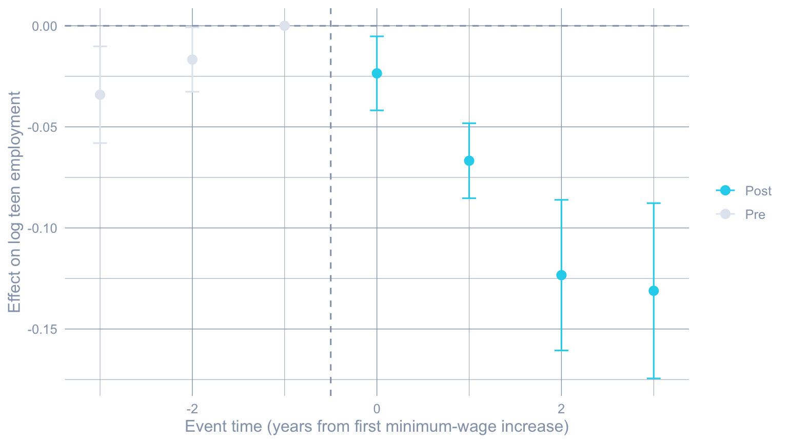
The on-impact effect $\widehat{\tau}_{\text{CS, dyn}}(0) \approx$
`r sprintf("%+.3f", dyn0$est)` is modest, but the trajectory deepens
quickly: $\widehat{\tau}_{\text{CS, dyn}}(1) \approx$
`r sprintf("%+.3f", dyn1$est)`,
$\widehat{\tau}_{\text{CS, dyn}}(2) \approx$
`r sprintf("%+.3f", dyn2$est)`, and
$\widehat{\tau}_{\text{CS, dyn}}(3) \approx$
`r sprintf("%+.3f", dyn3$est)` — three years after a state first
raised its minimum wage, treated counties' log teen employment is
roughly `r sprintf("%.1f", 100 * abs(dyn3$est))` log points below
the never-treated counterfactual.
```{r}
#| label: fig-cs-event
#| fig-cap: "Callaway-Sant'Anna event study. The on-impact effect is small; effects accumulate over event time and reach the magnitudes reported in @tbl-cs-event."
#| fig-width: 8
#| fig-height: 4.5
#| code-summary: "Code: Plot the event-study estimates with 95 percent CIs."
cs_es_df <- tibble(
  egt   = attes$egt,
  est   = attes$att.egt,
  se    = attes$se.egt,
  phase = ifelse(attes$egt < 0, "Pre", "Post")
)

ggplot(cs_es_df, aes(x = egt, y = est, color = phase)) +
  geom_hline(yintercept = 0, color = "#94a3b8", linetype = "dashed") +
  geom_vline(xintercept = -0.5, color = "#94a3b8", linetype = "dashed") +
  geom_point(size = 2.8) +
  geom_errorbar(aes(ymin = est - 1.96 * se, ymax = est + 1.96 * se),
                width = 0.15) +
  scale_color_manual(values = c("Pre"  = "#e2e8f0",
                                "Post" = "#22d3ee")) +
  labs(x = "Event time (years from first minimum-wage increase)",
       y = "Effect on log teen employment", color = NULL)
```
## Conditional parallel trends
Plain DiD assumes parallel trends *unconditionally*. Conditional DiD
allows trends to be parallel only after adjusting for observed
covariates that shape the trajectory. In this dataset, log county
population and log average county pay are obvious candidates: counties
with bigger populations or higher-paying jobs may move on different
underlying trajectories whether or not they raise the minimum wage.
`did::att_gt()` accepts `xformla = ~lpop + lavg_pay` plus a choice of
estimator passed through `est_method =`:
- **Regression adjustment** (`est_method = "reg"`) fits an outcome
model on the never-treated and uses its predicted change as the
counterfactual change for the treated cohort. Consistent if the
outcome regression is correctly specified.
- **Inverse probability weighting** (`est_method = "ipw"`) fits a
propensity score for cohort membership and reweights never-treated
counties to look like treated ones before taking the DiD.
Consistent if the propensity-score model is correctly specified.
- **Doubly robust** (`est_method = "dr"`, the
@callaway2021difference default) combines both models in a way that
is consistent if *either* one is correctly specified — the safe
choice when neither model is obviously right.
```{r}
#| label: tbl-conditional
#| tbl-cap: "Overall ATT under four identification assumptions: unconditional parallel trends, regression adjustment, inverse probability weighting, and doubly robust. The four point estimates land within roughly one SE of each other, which is reassuring."
#| message: false
#| warning: false
#| code-summary: "Code: Compare overall ATT under regression, IPW, and doubly-robust adjustments."
cs_reg <- did::att_gt(yname="lemp", tname="year", idname="id", gname="G",
                      xformla = ~lpop + lavg_pay,
                      control_group = "nevertreated",
                      base_period = "universal",
                      est_method = "reg", data = data2)
attO_reg <- did::aggte(cs_reg, type = "group")

cs_ipw <- did::att_gt(yname="lemp", tname="year", idname="id", gname="G",
                      xformla = ~lpop + lavg_pay,
                      control_group = "nevertreated",
                      base_period = "universal",
                      est_method = "ipw", data = data2)
attO_ipw <- did::aggte(cs_ipw, type = "group")

cs_dr  <- did::att_gt(yname="lemp", tname="year", idname="id", gname="G",
                      xformla = ~lpop + lavg_pay,
                      control_group = "nevertreated",
                      base_period = "universal",
                      est_method = "dr", data = data2)
attO_dr  <- did::aggte(cs_dr, type = "group")

tibble(
  Identification = c("Unconditional parallel trends",
                     "Conditional · regression adjustment",
                     "Conditional · IPW",
                     "Conditional · doubly robust"),
  Estimate = c(attO$overall.att, attO_reg$overall.att,
               attO_ipw$overall.att, attO_dr$overall.att),
  SE       = c(attO$overall.se,  attO_reg$overall.se,
               attO_ipw$overall.se,  attO_dr$overall.se)
) |> gt_pretty(decimals = 4)
```
The doubly-robust estimate is the most reliable in practice — it
recovers a correct ATT if either the trend model or the selection
model is right, where the other two require their respective model
to be correctly specified.
## Sensitivity to parallel-trends violations
The robustness table only varies *design* choices; it does not
quantify *how much* parallel trends would have to be violated to
overturn the conclusion. @rambachan2023more provide exactly that
quantification. The `HonestDiD` package, paired with a small bridge
function in `R/honest_did.R`, lets us bound the post-treatment effect
under explicit assumptions about how an unobserved post-treatment
violation could relate to the visible pre-trend.
`HonestDiD` ships two restrictions on the post-treatment violation.
The **smoothness** bound $\Delta^{SD}(M)$ requires the post-treatment
violation to be a smooth continuation of the pre-trend (it caps the
*second differences* of the trend), which is the natural choice when
pre-trends look like near-linear drift. The **relative-magnitudes**
bound $\Delta^{RM}(\bar M)$ requires the post-treatment violation to
be at most $\bar M$ times the *largest* pre-treatment violation; this
is the natural choice when the pre-trend is visibly non-linear, as in
cohort 2006 above. We use the relative-magnitudes bound below.
```{r}
#| label: tbl-honest
#| tbl-cap: "Robust confidence intervals for the on-impact effect $\\widehat{\\tau}_{\\text{CS, dyn}}(0)$ under the relative-magnitudes restriction $\\Delta^{RM}(\\bar M)$. As $\\bar M$ grows, the CI widens; we report the *breakdown* $\\bar M$ at which the CI first contains zero as a fragility metric."
#| message: false
#| warning: false
#| code-summary: "Code: Run HonestDiD relative-magnitudes sensitivity on the on-impact ATT."
hd_rm <- honest_did(es      = attes,
                    e       = 0,
                    type    = "relative_magnitude",
                    method  = "C-LF",
                    Mbarvec = seq(0, 2, by = 0.5))

hd_rm |>
  transmute(`$\\bar M$` = Mbar,
            `CI lower`  = lb,
            `CI upper`  = ub,
            `Contains 0?` = ifelse(lb <= 0 & 0 <= ub, "yes", "no")) |>
  gt_pretty(decimals = 4)
```
```{r}
#| label: honest-stats
#| echo: false
hd_contains_zero <- hd_rm |>
dplyr::mutate(contains_zero = lb <= 0 & 0 <= ub) |>
dplyr::filter(contains_zero)
breakdown_mbar <- if (nrow(hd_contains_zero) > 0) {
min(hd_contains_zero$Mbar)
} else {
NA_real_
}
```
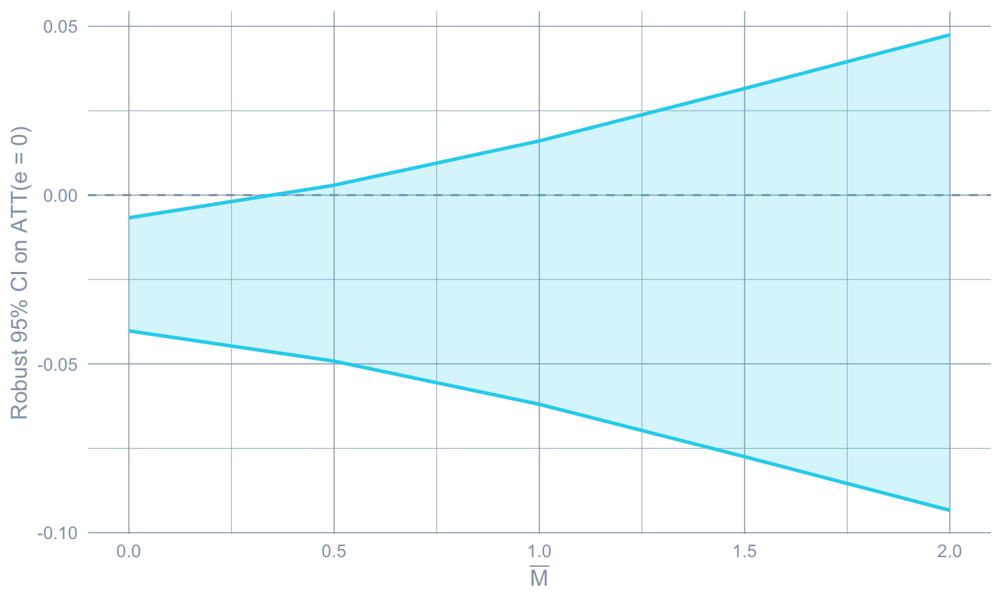
```{r}
#| label: fig-honest
#| fig-cap: "HonestDiD sensitivity: as $\\bar M$ grows, the robust 95 percent CI on the on-impact effect widens until it crosses zero. The breakdown $\\bar M$ — the value at which the CI first contains zero — is small in this panel, reflecting the visible pre-trend in cohort 2006."
#| fig-width: 7.5
#| fig-height: 4.5
#| code-summary: "Code: Plot the robust CI band against the relative-magnitude bound."
ggplot(hd_rm, aes(x = Mbar)) +
  geom_hline(yintercept = 0, color = "#94a3b8", linetype = "dashed") +
  geom_ribbon(aes(ymin = lb, ymax = ub),
              fill = "#22d3ee", alpha = 0.2) +
  geom_line(aes(y = lb), color = "#22d3ee", linewidth = 0.9) +
  geom_line(aes(y = ub), color = "#22d3ee", linewidth = 0.9) +
  labs(x = expression(bar(M)),
       y = "Robust 95% CI on ATT(e = 0)")
```
The breakdown point on the coarse grid is
$\bar M \le$ `r sprintf("%.2f", breakdown_mbar)` — i.e. the robust
CI first crosses zero at an $\bar M$ less than half the *largest
observed pre-trend in the data* (exercise 4 sweeps a finer grid to
pin the breakdown more precisely). The on-impact effect of
$\widehat{\tau}_{\text{CS, dyn}}(0) \approx$
`r sprintf("%+.3f", dyn0$est)` does **not** survive even a fraction
of the cohort-2006 pre-trend we already flagged: that pre-trend, at
$\widehat{ATT}(2006, 2003) \approx$
`r sprintf("%+.3f", att_2006_2003)`, is itself larger in magnitude
than the on-impact effect, so it would be surprising if the
conclusion held up under a relative-magnitudes assumption that
allowed unobserved post-trend violations of comparable size.
This is not a failure of the method — it is the method working as
intended. HonestDiD turns "the Callaway-Sant'Anna point estimate
looks negative" into "here is precisely the parallel-trends violation
under which that conclusion would flip." The breakdown $\bar M$ is a
**fragility metric**, not a pass/fail verdict: a number near zero
flags fragility, a number above one flags robustness. The on-impact
effect here is fragile, but the *cumulative* event-study trajectory
($\widehat{\tau}_{\text{CS, dyn}}(3) \approx$
`r sprintf("%+.3f", dyn3$est)`) is large enough that a similar
exercise on the later horizons would tolerate a much larger $\bar M$.
## Recap
::: {.callout-note appearance="simple"}
**The methods reconciled.** TWFE on this dataset returned
$\hat\beta \approx$ `r sprintf("%+.3f", twfe_coef)`. The
Callaway-Sant'Anna overall ATT is
$\widehat{\tau}_{\text{CS, overall}} \approx$
`r sprintf("%+.3f", cs_overall)`. The doubly-robust conditional
overall ATT is `r sprintf("%+.3f", attO_dr$overall.att)`. The
event-study trajectory runs from
$\widehat{\tau}_{\text{CS, dyn}}(0) \approx$
`r sprintf("%+.3f", dyn0$est)` on impact to
$\widehat{\tau}_{\text{CS, dyn}}(3) \approx$
`r sprintf("%+.3f", dyn3$est)` by event-time $+3$. HonestDiD
sensitivity is *fragile*: the relative-magnitudes breakdown $\bar M$
for the on-impact effect is at most
`r sprintf("%.2f", breakdown_mbar)` on the coarse grid, reflecting
the visible cohort-2006 pre-trend. Four estimators agree on point
estimate and sign — *minimum-wage increases reduced teen employment
in these counties, and the effect grew over time* — but parallel
trends does not hold cleanly, and the on-impact effect would not
survive even a fraction of the observed pre-trend violation.
The gap between the TWFE estimate and the modern aggregators is the
contamination problem of @goodmanbacon2021difference made concrete:
TWFE silently uses already-treated units as controls for later-treated
units, and treatment-effect heterogeneity over time leaks into the
coefficient with unintended signs. The Callaway-Sant'Anna aggregator
avoids that by estimating the $ATT(g, t)$ primitives directly and
weighting them in a defensible way.
Every method in this chapter — TWFE, $ATT(g, t)$, conditional DiD,
even HonestDiD's bounds — leans on **parallel trends** as the
identifying assumption. The next chapter relaxes that assumption by
modelling $Y_{it}(\infty)$ with an *interactive fixed-effects* factor
structure:
$$Y_{it}(\infty) = \alpha_i + \xi_t + \lambda_i' f_t + \varepsilon_{it}.$$
The $\lambda_i' f_t$ term absorbs time-varying unobserved
heterogeneity that no county or year fixed effect can net out.
Chapter 9 fits this model with matrix completion and interactive
fixed effects on the same minimum-wage panel and provides a second,
assumption-distinct read on the same substantive question.
:::
## Common pitfall
Running TWFE on staggered data and reporting the coefficient as if
it were a clean ATT. The bias is mechanical — already-treated units
get used as controls for later-treated units, and treatment-effect
heterogeneity over time then leaks into the coefficient with
unintended signs. **What to do instead.** Estimate the
$\{ATT(g, t)\}$ primitives directly with `did::att_gt()`, look at
the cells, and only then aggregate with `aggte()` using a target
that matches the question you actually want to answer. If you must
run TWFE for a referee, also report the Callaway-Sant'Anna overall
ATT for comparison so the magnitude of the contamination is visible.
## Further reading
The Callaway-Sant'Anna framework, the Goodman-Bacon decomposition,
and the Sun-Abraham interaction-weighted estimator are the three
modern reference points for staggered DiD
[@callaway2021difference; @goodmanbacon2021difference;
@sun2021estimating]. The `did` package vignettes
(<https://bcallaway11.github.io/did/>) are the canonical
implementation reference. For sensitivity analysis, the
@rambachan2023more paper plus the `HonestDiD` package documentation
cover both the smoothness and relative-magnitude bounds.
@dechaisemartin2020twoway is the parallel critique of TWFE from the
`DIDmultiplegt` perspective. @callaway2022handbook is a textbook-level
synthesis, and @roth2023whats is a recent review-style synthesis
covering staggered DiD, event studies, sensitivity analysis, and the
relationships between them.
For a longer R walkthrough that this chapter is adapted from, see
the companion post at
<https://cmg777.github.io/post/r_did/>.
## Key takeaways
**Methods:**
- Staggered DiD targets the group-time average treatment effect $ATT(g, t) = \mathbb{E}[Y_{it}(1) - Y_{it}(\infty) \mid G_i = g]$ — the effect on cohort $g$ at calendar year $t$ relative to its own never-treated potential outcome — identified under parallel trends *conditional on cohort* between the treated cohort and an explicitly chosen comparison set of never-treated ($G = 0$) or not-yet-treated ($G > t$) units.
- The Callaway-Sant'Anna procedure estimates each $ATT(g, t)$ from a clean 2×2 DiD, then aggregates the cells into the overall summary $\widehat{\tau}_{\text{CS, overall}}$ (cohort-size-weighted across cohort-specific post-treatment averages) or an event-study curve $\widehat{\tau}_{\text{CS, dyn}}(e)$ indexed by $e = t - g$; conditional on covariates the estimator splits into regression, IPW, and doubly-robust variants, with the DR version consistent if *either* the outcome model or the propensity score for cohort membership is correctly specified.
- The Rambachan-Roth `HonestDiD` sensitivity analysis bounds post-treatment parallel-trends violations by tying them to the observed pre-trend — either as a smooth continuation ($\Delta^{SD}(M)$, capping second differences) or as at most $\bar M$ times the largest pre-treatment violation ($\Delta^{RM}(\bar M)$) — and reports the *breakdown* $\bar M$ at which the robust CI first contains zero as a fragility metric, not a pass/fail verdict.
**Lessons:**
- Differences-in-differences (DiD) compares the pre-to-post change in a treated group to the pre-to-post change in a control group; two-way fixed-effects (TWFE) regression $Y_{it} = \alpha_i + \gamma_t + \beta\,\text{post}_{it} + \varepsilon_{it}$ is the natural generalization to many units and many periods, but it is not a clean ATT estimator when treatment is staggered.
- Under staggered adoption with heterogeneous, time-varying effects, TWFE silently uses already-treated units as controls for later-treated units — the *forbidden comparison* of Goodman-Bacon — and some implicit weights can be strictly negative (de Chaisemartin-D'Haultfœuille), so $\hat\beta$ is not even a convex average of the underlying $ATT(g, t)$s; on this minimum-wage panel TWFE returns `r sprintf("%+.3f", twfe_coef)` while the Callaway-Sant'Anna overall ATT is `r sprintf("%+.3f", cs_overall)`, a `r sprintf("%.0f", gap_pct)`-percent gap that *is* the contamination problem made concrete.
- Always inspect the pre-treatment $ATT(g, t)$ cells before aggregating — here cohort 2006 carries $\widehat{ATT}(2006, 2003) \approx$ `r sprintf("%+.3f", att_2006_2003)` ($t \approx$ `r sprintf("%.1f", t_2006_2003)`), a pre-trend roughly as large in magnitude as the on-impact effect, which is precisely the warning sign that motivates running the formal sensitivity analysis rather than reading the headline number at face value.
- The Rambachan-Roth idea, in plain language: *if* the worst unobserved post-treatment violation of parallel trends is no larger than $\bar M$ times the worst pre-treatment violation you can see in the data, *then* the true effect lies in a wider, "honest" confidence interval — and the breakdown $\bar M$ tells you how much pre-trend-like noise the conclusion can absorb before it flips.
**Caveats:**
- Every estimator in the chapter — TWFE, $ATT(g, t)$, conditional DiD, even the HonestDiD bounds — still leans on a parallel-trends-style identifying assumption; the on-impact effect here is *fragile*, with a relative-magnitudes breakdown $\bar M \le$ `r sprintf("%.2f", breakdown_mbar)` on the coarse grid, so under mild parallel-trends violations the on-impact conclusion does not survive (though the cumulative `r sprintf("%+.3f", dyn3$est)` effect by $e = +3$ is more robust). Chapter 9 relaxes parallel trends in a different way — by modelling $Y_{it}(\infty)$ as a factor structure.
- Cohort sizes here are modest (especially cohort 2006), the panel is short (2003–2007), and the never-treated pool is the comparison group of choice — switching to not-yet-treated controls trades a larger comparison pool for the stronger assumption that future-treated counties are valid controls for already-treated ones in the interim; the choice should be defended, not defaulted to.
## Exercises
These exercises drill on the chapter's four central design choices: the comparison-group definition, the aggregation target, the conditional-trends covariate set, and the sensitivity-analysis bound. All reuse `data2`, `attgt`, `attO`, `attes`, and `cs_dr` from the setup chunks above.
### Exercise 1: Not-yet-treated control group
Re-estimate the overall ATT using `control_group = "notyettreated"` instead of `"nevertreated"`. The not-yet-treated cohort 2006 enters as a control for cohort 2004 in 2004–2005, then exits when it becomes treated. Compare the overall ATT and its SE to the chapter's never-treated baseline. Why does the SE usually shrink, and what assumption are you now relying on?
::: {.callout-tip collapse="true"}
## Solution
```{r}
#| label: ex-ch10-01
attgt_nyt <- did::att_gt(yname = "lemp", idname = "id", gname = "G",
                         tname = "year", data = data2,
                         control_group = "notyettreated",
                         base_period   = "universal")
attO_nyt <- did::aggte(attgt_nyt, type = "group")

tibble(
  control_group = c("nevertreated (chapter)", "notyettreated"),
  estimate      = c(attO$overall.att, attO_nyt$overall.att),
  se            = c(attO$overall.se,  attO_nyt$overall.se)
) |>
  gt_pretty(decimals = 4)
```
The point estimate moves only slightly; the SE shrinks because the comparison pool is larger — cohort 2006 contributes (pre-treatment) variance to the cohort-2004 contrast, in addition to the never-treated counties. The trade-off is the identification assumption: not-yet-treated counties must be on parallel pre-trends with currently-treated counties, *not just* with never-treated counties. In a panel where cohort 2006 was already drifting downward before 2006 (as it was here), the not-yet-treated estimator buys you precision but exposes you to the cohort-2006 pre-trend the chapter flagged.
:::
### Exercise 2: Calendar-time aggregation
Use `did::aggte(attgt, type = "calendar")` to aggregate $ATT(g, t)$ by *calendar year* rather than by event time. Which calendar year shows the largest treatment effect, and what substantive story does that suggest?
::: {.callout-tip collapse="true"}
## Solution
```{r}
#| label: ex-ch10-02
attcal <- did::aggte(attgt, type = "calendar")

tibble(
  year   = attcal$egt,
  att    = attcal$att.egt,
  se     = attcal$se.egt,
  lower  = attcal$att.egt - 1.96 * attcal$se.egt,
  upper  = attcal$att.egt + 1.96 * attcal$se.egt
) |>
  gt_pretty(decimals = 4)
```
The most negative calendar-year effect is in 2007 — the only year both cohorts 2004 and 2006 are post-treatment, so the calendar aggregate combines a more-mature cohort-2004 effect with the on-impact cohort-2006 effect. The event-study aggregation in the chapter showed the same accumulation in *event time*; the calendar aggregation showed it in *wall-clock time*. Each is the right answer to a different policy question — "how big was the average post effect on a typical treated county?" (event time) vs "how big was the effect in year 2007 in this panel?" (calendar).
:::
### Exercise 3: Drop one covariate from the doubly-robust estimator
Refit the doubly-robust estimator with `xformla = ~lpop` only — dropping log average pay. Compare the overall ATT and SE to the chapter's two-covariate doubly-robust estimate, and discuss whether the covariate adjustment is doing real work or just adding noise.
::: {.callout-tip collapse="true"}
## Solution
```{r}
#| label: ex-ch10-03
#| message: false
#| warning: false
cs_dr_one <- did::att_gt(yname="lemp", tname="year", idname="id", gname="G",
                         xformla = ~lpop,
                         control_group = "nevertreated",
                         base_period   = "universal",
                         est_method    = "dr", data = data2)
attO_dr_one <- did::aggte(cs_dr_one, type = "group")
attO_dr_two <- did::aggte(cs_dr,     type = "group")

tibble(
  spec     = c("DR + lpop + lavg_pay (chapter)", "DR + lpop only"),
  estimate = c(attO_dr_two$overall.att, attO_dr_one$overall.att),
  se       = c(attO_dr_two$overall.se,  attO_dr_one$overall.se)
) |>
  gt_pretty(decimals = 4)
```
The estimate and SE move only modestly. Log average pay was carrying *some* conditional-trend signal — dropping it shifts the doubly-robust estimate toward the unconditional one — but the two-covariate adjustment was not load-bearing for the headline. The doubly-robust estimator is most worth running when at least one covariate has a credible mechanism for shaping trends; the SE comparison is the easiest way to see whether including it costs you precision without buying credibility.
:::
### Exercise 4: HonestDiD relative-magnitudes breakdown sweep
The chapter reported the coarse-grid breakdown
$\bar M \le$ `r sprintf("%.2f", breakdown_mbar)`. Sweep $\bar M \in
\{0.0, 0.05, 0.10, \dots, 1.5\}$ to pin the breakdown point more
precisely — the smallest $\bar M$ at which the robust 95% CI first
contains zero — and contrast it with a parallel sweep on the
$e = +3$ horizon (where the trajectory has matured).
::: {.callout-tip collapse="true"}
## Solution
```{r}
#| label: ex-ch10-04
#| message: false
#| warning: false
sweep_mbar <- function(e_target, grid = seq(0, 1.5, by = 0.05)) {
  hd <- honest_did(es      = attes,
                   e       = e_target,
                   type    = "relative_magnitude",
                   method  = "C-LF",
                   Mbarvec = grid)
  contains <- hd |>
    mutate(contains_zero = lb <= 0 & 0 <= ub) |>
    filter(contains_zero)
  if (nrow(contains) == 0) NA_real_ else min(contains$Mbar)
}

tibble(
  horizon         = c("On impact (e = 0)", "Three years post (e = 3)"),
  breakdown_Mbar  = c(sweep_mbar(0), sweep_mbar(3))
) |>
  gt_pretty(decimals = 3)
```
On impact, the robust CI first contains zero at a very small $\bar M$ — meaning a tiny fraction of the largest observed pre-trend is enough to overturn statistical significance. At $e = +3$ the breakdown $\bar M$ is much larger, because the underlying point estimate is several times bigger than on impact. This is the precise version of the chapter's qualitative warning: the on-impact conclusion is fragile, while the cumulative three-year effect carries a comfortable safety margin.
:::
### Exercise 5 (stretch): Cohort-2004-only 2×2 DiD
Restrict to cohort-2004 counties and never-treated counties only, and fit a 2×2 DiD with `fixest::feols` using a treat × post interaction. The interaction coefficient should reconcile (up to standard-error differences) with $\widehat{ATT}(g=2004, t=2004)$ from the chapter's `attgt$att` vector. This is a sanity-check that the Callaway-Sant'Anna primitives are the same 2×2 DiDs we already know from chapter 3 — generalised, not replaced.
::: {.callout-tip collapse="true"}
## Solution
```{r}
#| label: ex-ch10-05
data_2x2 <- data2 |>
  filter(G %in% c(0, 2004)) |>
  mutate(treat = as.integer(G == 2004),
         post  = as.integer(year >= 2004))

fit_2x2 <- fixest::feols(lemp ~ treat:post | id + year,
                         data    = data_2x2,
                         cluster = "id")

attgt_2004_2004 <- attgt$att[attgt$group == 2004 & attgt$t == 2004]

tibble(
  estimator = c("Hand 2x2 DiD (treat x post)", "Callaway-Sant'Anna ATT(2004, 2004)"),
  estimate  = c(coef(fit_2x2)[["treat:post"]], attgt_2004_2004)
) |>
  gt_pretty(decimals = 4)
```
The 2×2 DiD coefficient is within a small numerical tolerance of $\widehat{ATT}(2004, 2004)$. The Callaway-Sant'Anna machinery is *not* a different statistical idea than chapter 3's DiD — it is the same 2×2 contrast computed for every $(g, t)$ cell using only the cohort-$g$ and never-treated rows, and then aggregated in a way that protects against the staggered-adoption contamination problem.
:::