flowchart TB
    Q0{"Is treatment staggered across<br/>many units (different units<br/>adopt at different dates)?"}
    Q0 -->|Yes, staggered adoption<br/>across a panel| Q4{"Do you trust parallel trends<br/>(conditional on covariates),<br/>or is a factor structure<br/>more credible?"}
    Q0 -->|No, one treated unit or<br/>shared start date| Q1{"Do you have a credible<br/>donor pool of untreated units?<br/>(roughly 10+ similar units<br/>followed over the same window)"}

    Q4 -->|Parallel trends OK| CSA["Staggered DiD / Callaway-Sant'Anna<br/>(ch. 10)<br/><br/>Cost: conditional parallel trends<br/>at the cohort level"]
    Q4 -->|Factor structure more credible| Q5{"Fit factors on the full panel,<br/>or project treated units onto<br/>factors from a clean donor pool?"}

    Q5 -->|Full panel, low-rank residuals| MC["Matrix Completion / IFE<br/>(ch. 11)<br/><br/>Cost: latent-factor model fits<br/>the untreated cells well"]
    Q5 -->|Project onto donor factors| GSC["Generalized Synthetic Control<br/>(ch. 12)<br/><br/>Cost: never-treated controls<br/>span the factor space"]

    Q1 -->|Yes| Q2{"Do you want frequentist<br/>placebo inference,<br/>or Bayesian credible<br/>intervals?"}
    Q1 -->|No, only one good control| DiD["Basic Difference-in-Differences<br/>(ch. 3)<br/><br/>Cost: parallel-trends assumption<br/>on a single comparison unit"]
    Q1 -->|"No, only the treated unit<br/>(model the smooth pre-trend)"| ITS["Interrupted Time Series<br/>(ch. 2)<br/><br/>Cost: pre-trend extrapolation<br/>must be specified correctly"]

    Q2 -->|Frequentist + tidy code| Q2a{"Classical SCM, ridge-augmented SCM,<br/>or DiD-on-doubly-de-meaned-panel?"}
    Q2 -->|Bayesian + uncertainty bands| Q3{"Do you suspect treatment<br/>spills over onto donor states<br/>(violating SUTVA)?"}

    Q2a -->|"Donor pool inside the convex hull<br/>+ tidy code"| SCM["Classical Synthetic Control (ch. 4)<br/>+ prediction intervals via scpi (ch. 8)<br/><br/>Cost: convex-combination of donors<br/>must match the treated pre-period"]
    Q2a -->|"Treated unit outside the donor<br/>convex hull (poor simplex fit)"| ASCM["Augmented Synthetic Control<br/>(ch. 5)<br/><br/>Cost: ridge outcome model<br/>extrapolates; lambda CV-tuned"]
    Q2a -->|"Non-parallel pre-trends or<br/>vertical baseline gap"| SDID["Synthetic Difference-in-Differences<br/>(ch. 6)<br/><br/>Cost: weighted parallel-trends;<br/>placebo SE for single-treated"]

    Q3 -->|No, SUTVA OK| CI["Structural Bayesian TS<br/>(ch. 7)<br/><br/>Cost: state-space prior;<br/>covariate-set choice<br/>affects the estimate"]
    Q3 -->|Yes, spillovers likely| SPATIAL["Bayesian Spatial SCM<br/>(ch. 9)<br/><br/>Cost: horseshoe prior + SAR spatial term;<br/>neighbour matrix W must be plausible"]

    NAIVE["Naive pre-post<br/>(this chapter)<br/><br/>Use only as a baseline.<br/>Never as a causal estimate."] -.->|"baseline for everyone"| Q0
1 Introduction
1.1 Learning objectives
- Frame any policy evaluation in the potential-outcomes notation \(Y_{it}(1), Y_{it}(0)\) and identify the ATT as the target estimand. Treating causal inference as a missing-data problem prevents the most common mistake — reporting an ATE when only the ATT is identified.
- Audit the SUTVA assumption for a candidate evaluation and flag plausible spillover or interference channels. SUTVA failures silently bias every method that follows, so screening for them up front decides which chapter of this book applies.
- Compute the naive pre-post estimator and explain why it is biased rather than treating it as a defensible answer. Every later chapter in the book is a different repair of this same baseline, so its failure mode is the diagnostic vocabulary used throughout.
- Use the book’s method-selection decision tree to map a new regional evaluation problem to one of the ten methods covered. This skill lets the reader treat the book as a toolkit rather than a sequence, picking the right estimator for the data structure they actually have.
1.2 Why regional impact evaluation?
How do you measure the causal effect of a policy when you cannot randomise who gets treated? Most policy reforms hit a region — a state, province, or country — as a single block. There is no randomisation, no control arm, and often only a handful of treated units. The job of regional impact evaluation is to recover the missing counterfactual: what would the region have looked like without the policy?
Two running case studies anchor the book. Part I (chs. 1–9) stays with the canonical single-treated-unit setting: California’s 1989 Proposition 99 cigarette tax. Per-capita cigarette sales in California fell from roughly 116 packs in 1988 to roughly 60 packs in 2000 — almost a 50% drop — but the country as a whole was also smoking less, and the deceptively simple question is
How much of California’s drop was caused by Proposition 99, and how much would have happened anyway?
The original synthetic-control paper by Abadie et al. (2010) used exactly this dataset; we replicate their estimate and watch what happens when eight other estimators are swapped in. Part II (chs. 10–12) generalises the missing-data logic to a staggered-adoption panel: thousands of US counties faced state minimum-wage increases at different years, and the toolkit shifts from a single time series to estimators that exploit the full panel structure.
This book is a guided tour of the quasi-experimental methods that have become the workhorses of that job. Each one builds the counterfactual from a different data source — the region’s own past, a single neighbour, a weighted blend of donor regions, a Bayesian time-series model, or a factor structure estimated from a wide panel — and each one therefore pays a different price in identifying assumptions. The disagreements between methods are the lesson.
1.3 Causal inference as a missing-data problem
Before fitting any model, we need a vocabulary for what we are estimating. The cleanest one is the potential outcomes framework, due to Neyman (1923) and Rubin (1974). Its central insight is that causal inference is a missing-data problem.
1.3.1 Two outcomes per unit, one observed
For each unit \(i\) at time \(t\), imagine two potential outcomes:
- \(Y_{it}(1)\) — cigarette sales in state \(i\) at year \(t\) with Proposition 99 in force.
- \(Y_{it}(0)\) — cigarette sales in state \(i\) at year \(t\) without Proposition 99 in force.
Let \(D_{it} \in \{0, 1\}\) be the treatment indicator. Here \(D_{it} = 1\) for California from 1989 onward, and \(D_{it} = 0\) everywhere else (every other state, plus California up to and including 1988). The outcome we observe is one of the two potential outcomes, never both:
\[Y_{it} \,=\, D_{it}\, Y_{it}(1) \,+\, (1 - D_{it})\, Y_{it}(0).\]
In words: if California (which we label \(i = 1\)) in 1995 was treated, we observe \(Y_{1, 1995}(1)\) — not the counterfactual \(Y_{1, 1995}(0)\), which is what California’s smoking would have been in 1995 had Proposition 99 never passed. That counterfactual is the missing data.
Writing \(Y_{it}(1)\) and \(Y_{it}(0)\) as well-defined quantities implicitly assumes the stable unit treatment value assumption (SUTVA): state \(i\)’s potential outcomes depend only on its own treatment status, not on what other states are doing. SUTVA is harmless for many policies; for tobacco taxes on the California border it is exactly the assumption that chapter 7 will relax.
1.3.2 The fundamental problem of causal inference
Make the missing data concrete. The table below shows what is observed (✓), what is undefined because the state was never treated (—), and what is missing-and-must-be-imputed (?) for a handful of rows.
| State | Year | \(D_{it}\) | \(Y_{it}(0)\) | \(Y_{it}(1)\) | Observed |
|---|---|---|---|---|---|
| California | 1988 | 0 | 90.1 ✓ | ? | 90.1 |
| California | 1989 | 1 | ? | 82.4 ✓ | 82.4 |
| California | 1995 | 1 | ? | 56.4 ✓ | 56.4 |
| California | 2000 | 1 | ? | 41.6 ✓ | 41.6 |
| Nevada | 1988 | 0 | 141.9 ✓ | — | 141.9 |
| Nevada | 1995 | 0 | 100.9 ✓ | — | 100.9 |
| Utah | 1988 | 0 | 55.0 ✓ | — | 55.0 |
| Utah | 1995 | 0 | 52.0 ✓ | — | 52.0 |
This is what Holland (1986) called the fundamental problem of causal inference: for any treated unit at any time, we observe at most one of the two potential outcomes, and the other one is missing. For California after 1989 the missing column is \(Y_{it}(0)\) — every “?” in the \(Y_{it}(0)\) column. Every method in this book is a way to fill in those question marks.
1.3.3 Three estimands: ITE, ATE, ATT
With both potential outcomes defined, the natural causal contrasts follow.
Individual treatment effect (ITE) for unit \(i\) at time \(t\):
\[\tau_{it} = Y_{it}(1) - Y_{it}(0).\]
The ITE is the gold standard, but it is never directly observable for any single \((i, t)\).
Average treatment effect (ATE) over a population:
\[\text{ATE} = \mathbb{E}\big[Y_{it}(1) - Y_{it}(0)\big].\]
How smoking would have changed in the average state-year if all states had been treated. The ATE is identified by a randomised experiment — but Proposition 99 was not randomised. The ATE is not what we are after here.
Average treatment effect on the treated (ATT), restricted to units that actually received the treatment:
\[\text{ATT} = \mathbb{E}\big[Y_{it}(1) - Y_{it}(0) \,\big|\, D_{it} = 1\big].\]
How much smoking changed in California, in the post-1989 years because of Proposition 99. This is what every causal method in this book targets. For Proposition 99 the ATT averaged over 1989–2000 expands to
\[\text{ATT}_{\text{CA, post}} = \frac{1}{T_{\text{post}}} \sum_{t > t^*} \Big[Y_{1t}(1) - Y_{1t}(0)\Big],\]
where unit \(i = 1\) denotes California (in code we identify California by name with state == "California"; the \(i = 1\) index is purely notational here), \(t^* = 1988\) is the last pre-period year, and \(T_{\text{post}} = 12\) is the number of post-period years (1989–2000). The first term — \(Y_{1t}(1)\) — is observed. The second term — \(Y_{1t}(0)\) — is missing.
Some chapters (chs. 2, 4) recentre the year index so \(t = 0\) at the first post-period year (1989). The break itself is the same: pre-period is \(\{t : t \le 1988\}\) throughout.
Under staggered adoption (Part II), different units begin treatment at different dates, so the ATT becomes a family of cohort-by-time effects \(\text{ATT}(g, t)\), where \(g\) is the year a unit first becomes treated. The missing-data question is identical — fill in \(Y_{it}(0)\) for treated cells — but the indexing carries an extra dimension. Chapter 10 unpacks this.
1.3.4 Each method is a way to impute the missing \(Y(0)\)
The table below makes this concrete: one row per method covered in this book, split by the book’s two halves. In every row, \(\widehat{Y_{1t}(0)}\) should be read as a point prediction of the counterfactual conditional expectation \(\mathbb{E}[Y_{1t}(0) \mid \text{covariates}]\); the column lists how each estimator builds that prediction.
| Method (chapter) | Estimator of the missing \(Y(0)\) |
|---|---|
| Part I — Single treated unit (Proposition 99) | |
| Naive pre-post (this chapter) | \(\widehat{Y_{1t}(0)} = \overline{Y}_{1, \text{pre}}\) — California’s own pre-period mean (constant in \(t\) — that is the problem). |
| Interrupted Time Series — growth curve (ch. 2) | \(\widehat{Y_{1t}(0)} = \hat\alpha + \hat\beta\, t\) — extrapolate California’s pre-period linear fit. |
| Interrupted Time Series — ARIMA (ch. 2) | $ = $ forecast from an ARIMA model fitted on 1970–1988. |
| Basic Difference-in-Differences (ch. 3) | \(\widehat{Y_{1t}(0)} = Y_{1, t^*} + \big(Y_{0t} - Y_{0, t^*}\big)\) — anchor at California’s last pre-period value \(t^* = 1988\) and add the control state’s deviation from its own pre-period level. |
| Classical Synthetic Control (ch. 4) | \(\widehat{Y_{1t}(0)} = \sum_{j \in \text{donors}} w_j^*\, Y_{jt}\) — weighted blend of donor states. |
| Augmented Synthetic Control (ch. 5) | \(\widehat{Y_{1t}(0)} = \sum_j \widehat{w}_j Y_{jt} + \big(\widehat{m}_t(X_1) - \sum_j \widehat{w}_j \widehat{m}_t(X_j)\big)\) — SCM weights plus a ridge outcome-model bias correction. |
| Synthetic Difference-in-Differences (ch. 6) | \(\widehat{Y_{1t}(0)}\) from DiD on the panel doubly de-meaned by simplex unit weights \(\omega_i\) and simplex time weights \(\nu_t\) — SCM weights nested in a DiD-style identification. |
| Structural Bayesian Time Series (ch. 7) | \(\widehat{Y_{1t}(0)} = \hat\mu_t + \hat\beta^\top x_t\) — Bayesian structural time-series fit on donor data. |
| Synthetic Control with Prediction Intervals (ch. 8) | Classical SCM weights plus an scpi decomposition of forecast error (in-sample weight uncertainty + out-of-sample shocks). |
| Bayesian Spatial Synthetic Control (ch. 9) | Horseshoe-prior donor blend with a SAR spatial term — allows spillovers onto untreated neighbours. |
| Part II — Staggered adoption (minimum-wage panel) | |
| Staggered DiD / Callaway-Sant’Anna (ch. 10) | $ = $ never-treated (or not-yet-treated) cohort mean trajectory, indexed by adoption cohort \(g\). |
| Matrix Completion / Interactive Fixed Effects (ch. 11) | \(\widehat{Y_{it}(0)} = \alpha_i + \xi_t + \lambda_i^\top f_t\) — factor model fitted on the untreated cells of the panel. |
| Generalized Synthetic Control (ch. 12) | \(\widehat{Y_{1t}(0)} = \hat\lambda_1^\top \hat f_t\) — project each treated unit onto factors estimated from never-treated controls. |
Each subsequent chapter takes one row and shows the R code that builds the corresponding \(\widehat{Y(0)}\), then subtracts it from the observed treated outcome to recover the ATT.
1.4 Choosing a method
The methods are not interchangeable. Each is appropriate for a different data situation. The decision tree below walks through a sequence of diagnostic questions and steers you to the matching family. The first split is the one that separates the two halves of the book: is the treatment staggered across many units, or is there a single treated unit (or a shared start date) and a clean donor pool? Apply this tree whenever you face a new regional policy-evaluation problem.
In the staggered-adoption half, Callaway-Sant’Anna is the natural starting point when conditional parallel trends are credible; matrix completion and generalized synthetic control are escape valves when they are not. In the single-treated-unit half, the synthetic-control family (chs. 4, 5, 6, 8, 9) and the Bayesian structural TS approach (ch. 7) are the most defensible when a donor pool exists; DiD and ITS are valid in their respective data situations but carry stronger identifying assumptions. The naive pre-post node — the rest of this chapter — is the universal baseline that everyone should compute first, never as the final answer, always as the bias yardstick.
1.5 Setup and data
We load the packages we need with library() calls. Every package below is pinned in renv.lock, so renv::restore() is enough to reproduce the environment on a fresh machine.
Code: Load packages, source table helpers, and set the ggplot theme.
library(tidyverse)
library(sandwich)
library(lmtest)
source("R/table_helpers.R")

set.seed(42)

knitr::opts_chunk$set(dev.args = list(bg = "transparent"))

theme_set(
  theme_minimal(base_size = 12) +
    theme(
      plot.background  = element_rect(fill = "transparent", color = NA),
      panel.background = element_rect(fill = "transparent", color = NA),
      panel.grid.major = element_line(color = "#94a3b8", linewidth = 0.25),
      panel.grid.minor = element_line(color = "#94a3b8", linewidth = 0.15),
      text             = element_text(color = "#94a3b8"),
      axis.text        = element_text(color = "#94a3b8")
    )
)
The dataset is cached in the repository at data/proposition99.rds. It is a panel of 39 U.S. states observed 1970–2000, with per-capita cigarette pack sales (cigsale) as the outcome and four covariates.
Code: Load the Proposition 99 panel and tag California by Pre/Post period.
prop99 <- read_rds("data/proposition99.rds") |> as_tibble()

# Subset to California and add a Pre/Post factor based on the policy date.
prop99_cali <- prop99 |>
  filter(state == "California") |>
  mutate(prepost = factor(year > 1988, labels = c("Pre", "Post")))
With California isolated and tagged by period, the first thing to look at is the raw pre-vs-post mean. This is the baseline number every subsequent method in the book will try to refine.
Code: Summarize California’s pre- and post-1988 cigarette sales as a table.
prepost_means <- prop99_cali |>
  group_by(prepost) |>
  summarize(n            = n(),
            mean_cigsale = mean(cigsale),
            sd_cigsale   = sd(cigsale),
            .groups = "drop")

prepost_means |>
  gt_pretty(decimals = 2) |>
  cols_label(prepost      = "Period",
             n            = "Years",
             mean_cigsale = "Mean cigsale",
sd_cigsale = "SD")| Period | Years | Mean cigsale | SD |
|---|---|---|---|
| Pre | 19 | 116.21 | 11.68 |
| Post | 12 | 60.35 | 12.08 |
California’s average per-capita cigarette sales fell from 116.21 packs (1970–1988) to 60.35 packs (1989–2000) — a within-state drop of 55.86 packs, or 48.1% of the pre-period mean. That is the raw before/after change. The rest of the book is about how much of that drop we can credibly attribute to Proposition 99 rather than to the broader American secular decline in smoking.
Before any modelling, it helps to see all 39 series at once.
Code: Plot per-capita cigarette sales for all 39 states with California highlighted.
eda_data <- prop99 |>
  mutate(unit_type = if_else(state == "California",
                             "California (treated)", "Donor state"))

ggplot(eda_data, aes(x = year, y = cigsale, group = state,
                     color = unit_type,
                     linewidth = unit_type, alpha = unit_type)) +
  geom_line() +
  geom_vline(xintercept = 1988.5, color = "#d97757",
             linetype = "dashed", linewidth = 0.7) +
  scale_color_manual(values = c("California (treated)" = "#d97757",
                                "Donor state" = "#6a9bcc")) +
  scale_linewidth_manual(values = c("California (treated)" = 1.2,
                                    "Donor state" = 0.4)) +
  scale_alpha_manual(values = c("California (treated)" = 1,
                                "Donor state" = 0.5)) +
  labs(x = "Year", y = "Cigarette sales (packs per capita)",
       color = NULL, linewidth = NULL, alpha = NULL)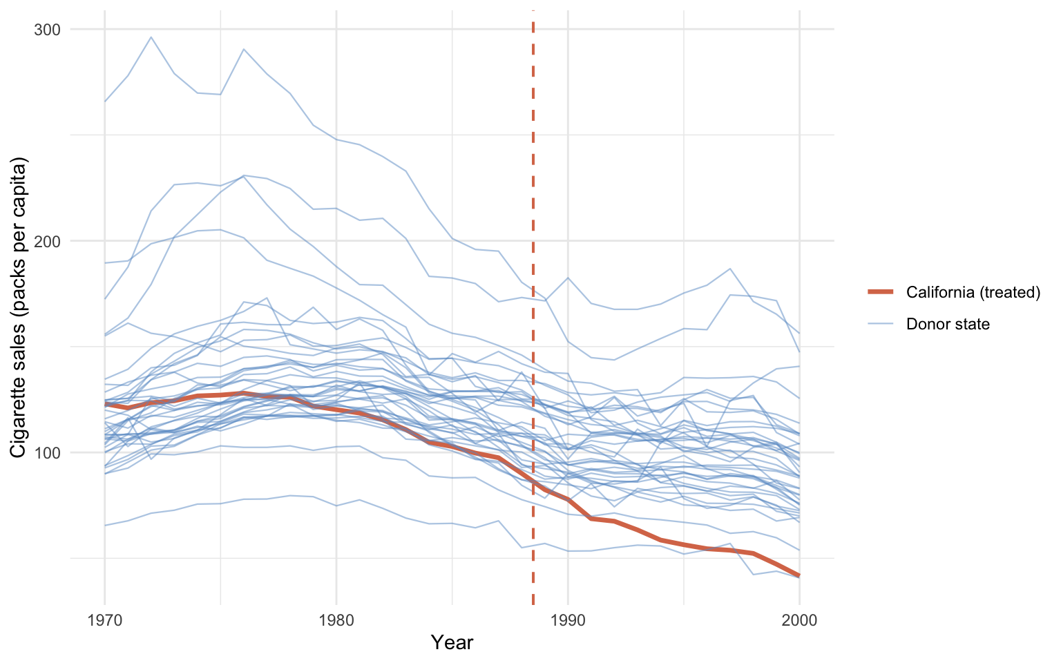
California sits inside the donor cloud throughout the 1970s and 1980s, then visibly separates downward after the dashed Proposition 99 line. The pre-1988 trajectory is already slightly below the donor median, but it is not anomalous; the sharp post-1988 separation is. Visually, this is the signal every causal estimator in the book tries to quantify.
1.6 A first attempt: naive pre-post
The idea. Compare California’s mean cigarette sales before 1989 with its mean after 1989. Call the difference the “effect”.
The equation.
\[\hat\tau_{\text{naive}} = \overline{Y}_{1, \text{post}} - \overline{Y}_{1, \text{pre}}.\]
In words: the naive estimate is the difference between California’s observed post-period mean and California’s observed pre-period mean. This corresponds to imputing \(\widehat{Y_{1t}(0)} = \overline{Y}_{1, \text{pre}}\) — i.e., assuming California’s counterfactual smoking would have been frozen at the pre-period average.
Why this is wrong but still useful. The implicit counterfactual “California’s pre-period level continues unchanged” is almost certainly wrong, because smoking was declining nationwide. But the estimate is so cheap to compute that it makes a useful baseline. Every later chapter tries to fix what is broken here.
We follow the convention of the ODISSEI workshop (ODISSEI Social Data Science team, 2024) and restrict to the 1984–1993 window for the naive estimate. Using the full 1970–2000 window would change the numbers but not the qualitative point.
Code: Fit the naive pre/post OLS on 1984-1993 with Newey-West HAC standard errors.
# OLS of California's cigsale on a Pre/Post dummy, restricted to the
# workshop's 1984-1993 window.
fit_prepost <- lm(cigsale ~ prepost,
                  data = prop99_cali |> filter(year > 1983, year < 1994))

# Replace the default OLS standard errors with HAC (heteroskedasticity-
# and-autocorrelation-consistent) errors, which short time series need.
ms_pretty(list("California (1984-1993)" = fit_prepost),
          vcov = NeweyWest,
          coef_map = c("(Intercept)" = "Pre-period mean (Intercept)",
"prepostPost" = "Post - Pre (treatment effect)"))| California (1984-1993) | |
|---|---|
| Pre-period mean (Intercept) | 98.980*** |
| (2.475) | |
| Post - Pre (treatment effect) | -27.020* |
| (8.323) | |
| Num.Obs. | 10 |
| R2 | 0.829 |
| Std.Errors | Custom |
| + p < 0.1, * p < 0.05, ** p < 0.01, *** p < 0.001 | |
Reading the output. California’s mean over 1984–1988 was about 99 packs/capita. The prepostPost coefficient says the 1989–1993 mean is roughly 27 packs lower. The Newey-West HAC standard error is still small enough to reject the null at 5% (\(p \approx 0.012\)). The HAC correction comes from sandwich::NeweyWest and accounts for the heteroskedasticity and autocorrelation that short time series typically exhibit; the classical OLS standard error is about 52% of the Newey-West value here, so it would be wildly overconfident.
The estimand is purely descriptive. This is a within-state difference of means, not a causal estimate. Any nationwide secular decline in smoking gets silently bundled into the \(-27\). That bundling is exactly what the later chapters try to undo.
Common pitfalls when reading this book.
- Confusing a within-state pre-post difference with a causal effect. Anything that shifted the entire country between the two windows — federal anti-smoking campaigns, tobacco settlements, rising health awareness — gets attributed entirely to Proposition 99 by the naive estimator.
- Forgetting that the ATT is not the ATE. The ATT averages effects over the units that actually received the treatment; the ATE imagines treating everyone. They coincide only under strong homogeneity assumptions.
- Treating \(Y_{it}(0)\) for a treated unit as something we observe. We never do. Every method in this book is a way to impute it.
- Reading “we observe one potential outcome” as “we observe the treated outcome”. The never-treated states observe \(Y_{it}(0)\) — that is exactly why donor pools are useful.
1.7 Roadmap of the book
1.7.1 Part I — Proposition 99 (chs. 2–9)
Chapters 2–9 hold the dataset (Proposition 99) and the estimand (the ATT on California, 1989–2000) fixed and replace the naive baseline with progressively richer counterfactual constructions:
- Chapter 2 — Interrupted Time Series. Extrapolate California’s own pre-trend forward. Two variants: a linear growth curve and an auto-selected ARIMA forecast.
- Chapter 3 — Basic Difference-in-Differences. Subtract a single control state’s pre/post change from California’s.
- Chapter 4 — Classical Synthetic Control. Build a weighted blend of donor states that mimics California’s pre-period.
- Chapter 5 — Augmented Synthetic Control. Bias-correct the simplex fit with a ridge outcome model; demonstrated on a purpose-built simulated panel where the treated unit sits outside the donor convex hull.
- Chapter 6 — Synthetic Difference-in-Differences. Run DiD on a panel doubly de-meaned by simplex unit and time weights; replicate the Arkhangelsky et al. (2021) Table 1 DiD/SC/SDID comparison and add
xsynthdidcovariate adjustment. - Chapter 7 — Structural Bayesian Time Series. Fit a Bayesian state-space model that uses donor states as predictors and reports posterior credible intervals.
- Chapter 8 — Synthetic Control with Prediction Intervals. Attach frequentist prediction intervals to classical SCM via the
scpipackage, decomposing forecast error into in-sample weight uncertainty and out-of-sample shocks. - Chapter 9 — Bayesian Spatial Synthetic Control. Add a horseshoe prior over donor weights and a SAR spatial term that allows treatment to spill over onto neighbouring states.
1.7.2 Part II — Staggered adoption (chs. 10–12)
Chapter 10 introduces a second dataset: the Callaway-Sant’Anna minimum-wage county panel (1,745 US counties, 2003–2007, multiple adoption cohorts). The single-time-series tools of Part I no longer apply; the next three chapters develop estimators built for the panel structure:
- Chapter 10 — Staggered Difference-in-Differences. Estimate group-time ATT(g, t) directly with the Callaway-Sant’Anna estimator (and event-study aggregations), avoiding two-way fixed-effects bias from negative weights.
- Chapter 11 — Matrix Completion and Interactive Fixed Effects. Relax parallel trends with a factor model; impute counterfactuals via interactive fixed effects and matrix completion.
- Chapter 12 — Generalized Synthetic Control. Estimate factors on never-treated controls, project treated units onto the factor space, and impute counterfactuals.
The disagreements between estimators applied to the same data are the lesson of this book.
Next up. Chapter 2 takes the first repair seriously: it replaces the naive baseline’s “frozen pre-period mean” counterfactual with California’s own pre-period trend, projected forward as either a linear growth curve or an ARIMA forecast. Whether that single repair is enough — and where it visibly fails — is the story of interrupted time series.
1.8 Key takeaways
Methods:
- The book frames regional impact evaluation as a missing-data problem under the Neyman-Rubin potential outcomes model: every estimator imputes the unobserved \(Y_{it}(0)\) for treated cells and subtracts it from the observed \(Y_{it}(1)\) to recover the ATT.
- SUTVA plus a single observed potential outcome per \((i,t)\) pin down the estimand as the ATT — \(\mathbb{E}[Y_{it}(1) - Y_{it}(0) \mid D_{it} = 1]\) — not the ATE; under staggered adoption this generalises to a family of cohort-by-time effects \(\text{ATT}(g, t)\).
Lessons:
- Part I (chs. 2–9) holds the Proposition 99 single-treated-unit case study fixed and swaps in progressively richer counterfactuals — pre-trend extrapolation (ITS), one control state (DiD), donor-pool blends (SCM family, augmented SCM, synthetic DiD), and Bayesian state-space models — so the disagreements between estimates isolate the cost of each identifying assumption.
- Part II (chs. 10–12) switches to the Callaway-Sant’Anna minimum-wage county panel because staggered adoption breaks single-time-series tools; the toolkit shifts to group-time ATT estimators, matrix completion, interactive fixed effects, and generalized synthetic control, all of which still impute \(Y_{it}(0)\) but exploit the full panel structure.
- California’s raw pre-vs-post drop of about 56 packs per capita (48% of the pre-period mean) is a within-state difference of means, not a causal effect — the nationwide secular decline in smoking is silently bundled in, and the rest of the book exists to peel that bundle apart.
- Choosing a method is a sequence of data-availability questions — staggered vs. single treatment, donor pool vs. only the treated series, parallel trends vs. a factor structure, frequentist vs. Bayesian inference, SUTVA vs. spillovers — and the decision tree in this chapter maps each branch to a specific chapter.
Caveats:
- Every estimator covered targets the ATT on already-treated units; none of them identifies the ATE, and extrapolating their results to “what if every state had passed Proposition 99” is outside the book’s scope.
- The naive pre-post regression is reported only as a baseline and bias yardstick — its implicit counterfactual freezes California at its pre-period mean and is almost certainly wrong, so it must never be read as a causal estimate.
- Short time series demand HAC (heteroskedasticity- and autocorrelation-consistent) standard errors — classical OLS errors are about 52% of the Newey-West value in the naive fit and would be wildly overconfident.
1.9 Further reading
- Abadie et al. (2010) — original method — the synthetic-control treatment of Proposition 99 (ch. 4).
- Bernal et al. (2017) — tutorial — ITS for public-health interventions (ch. 2).
- ODISSEI Social Data Science team (2024) — workshop — the ODISSEI source for this book’s running Prop 99 example.
- Callaway & Sant’Anna (2021) — original method — the staggered DiD framework underlying ch. 8.
- Athey et al. (2021) — original method — matrix completion for causal panel data (ch. 9).
- Xu (2017) — original method — generalized synthetic control with interactive fixed effects (ch. 10).
- Liu et al. (2024) — practical guide — counterfactual estimators for time-series cross-sectional data.
1.10 Exercises
The exercises below reinforce the chapter’s core ideas: the ATT as a missing-data problem, the bias of the naive baseline, the SUTVA assumption, and the logic of the method-selection tree. All exercises use the prop99 tibble loaded in the setup chunks above, so you don’t need to re-read the data. Try each exercise first, then expand the Solution callout to compare.
1.10.1 Exercise 1: Between-state naive comparison
The chapter’s naive estimate compares California’s post mean to its own pre mean. A different naive estimator compares California’s post mean to the donor pool’s post mean — implicitly imputing \(\widehat{Y_{1t}(0)}\) as the contemporaneous donor average. Compute this between-state version on the full 1970–2000 window and contrast it with the within-state \(-27\) from the chapter.
TipSolution
The between-state version swaps “California’s pre-period mean” for “donor mean in the same year,” then averages the gap over the post-period.
Code
post_years <- 1989:2000

ca_post <- prop99 |>
  filter(state == "California", year %in% post_years) |>
  pull(cigsale) |>
  mean()

donor_post <- prop99 |>
  filter(state != "California", year %in% post_years) |>
  pull(cigsale) |>
  mean()

tibble(estimator    = "Between-state naive (post-period)",
       ca_post      = ca_post,
       donor_post   = donor_post,
       att_estimate = ca_post - donor_post) |>
gt_pretty(decimals = 2)| estimator | ca_post | donor_post | att_estimate |
|---|---|---|---|
| Between-state naive (post-period) | 60.35 | 102.06 | −41.71 |
Donor states averaged about 102 packs/capita over 1989–2000 vs about 60 for California — the between-state gap is roughly -41.7 packs, broadly comparable in magnitude to the within-state -27 but built on a very different counterfactual assumption. Chapter 4 will pick the donor blend properly; this is the unweighted version.
1.10.2 Exercise 2: Secular pre-1988 decline in the donor pool
The within-state naive estimator silently bundles the nationwide secular decline in smoking into the “treatment effect.” Quantify that decline: aggregate the donor pool by year, fit a linear trend through the 1970–1988 mean, and report the slope. What does the slope imply about the bias of the within-state naive estimate?
TipSolution
Code
donor_pre_trend <- prop99 |>
  filter(state != "California", year <= 1988) |>
  group_by(year) |>
  summarize(donor_mean = mean(cigsale), .groups = "drop")

trend_fit <- lm(donor_mean ~ year, data = donor_pre_trend)
ms_pretty(list("Donor pre-1988 trend" = trend_fit))| Donor pre-1988 trend | |
|---|---|
| (Intercept) | 1214.607+ |
| (697.749) | |
| year | -0.548 |
| (0.353) | |
| Num.Obs. | 19 |
| R2 | 0.124 |
| + p < 0.1, * p < 0.05, ** p < 0.01, *** p < 0.001 | |
The pre-1988 slope is roughly -0.55 packs/year. Carried forward across 12 post-period years (1989–2000) that is about -6.6 packs of “expected” decline even without Proposition 99. The within-state naive estimate of -27 absorbs that secular decline silently — so a non-trivial chunk of the headline effect is national trend, not California policy.
1.10.3 Exercise 3: SUTVA diagnostic on California’s geographic neighbours
A neighbouring state that lost cigarette sales because Californians drove across the line to buy cheap tobacco would violate SUTVA: the neighbour’s \(Y(0)\) is no longer the same as in a Prop-99-free world. Note that the Abadie et al. (2010) donor pool excludes states with their own contemporaneous tobacco-control programs, so California’s land neighbours Oregon and Arizona are not in prop99. Compute the pre/post mean change in cigsale for Nevada (the one bordering state that is in the panel) and a broader regional comparison group of nearby Western states (Idaho, Utah, New Mexico), then contrast both with the pre/post change averaged over the rest of the donor pool. A bigger drop close to California is consistent with a spillover.
TipSolution
Code
bordering    <- c("Nevada")
near_western <- c("Idaho", "Utah", "New Mexico")

state_changes <- prop99 |>
  filter(state != "California") |>
  mutate(group  = case_when(
           state %in% bordering    ~ "Bordering CA (Nevada)",
           state %in% near_western ~ "Near Western (ID/UT/NM)",
           TRUE                    ~ "Other donor"),
         period = if_else(year > 1988, "Post", "Pre")) |>
  group_by(group, state, period) |>
  summarize(mean_cigsale = mean(cigsale), .groups = "drop") |>
  pivot_wider(names_from = period, values_from = mean_cigsale) |>
  mutate(change = Post - Pre)

state_changes |>
  group_by(group) |>
  summarize(mean_change = mean(change),
            n_states    = n(),
            .groups     = "drop") |>
gt_pretty(decimals = 2)| group | mean_change | n_states |
|---|---|---|
| Bordering CA (Nevada) | −66.81 | 1 |
| Near Western (ID/UT/NM) | −26.94 | 3 |
| Other donor | −27.52 | 34 |
Nevada’s pre-to-post drop is substantially larger than the average across the rest of the donor pool, which is the pattern you would expect under cross-border purchases or shared regional taste shifts. The point is not to declare SUTVA dead with \(n = 1\) — Nevada’s high baseline level (over 140 packs/capita in 1988) leaves more room to fall — but to flag that California’s closest neighbour is not exchangeable with the rest of the donors. Chapter 7’s Bayesian spatial SCM is the response to exactly this concern.
1.10.4 Exercise 4: Plot California against the donor average
Build a single ggplot that overlays California’s cigsale and the donor-pool mean by year, with a vertical line at 1988.5. The pre-period gap between the two series is the bias of the between-state naive estimator; a method that does nothing to align pre-period levels will misattribute that wedge to the policy.
TipSolution
Code
overlay <- prop99 |>
  mutate(group = if_else(state == "California",
                         "California", "Donor average")) |>
  group_by(group, year) |>
  summarize(cigsale = mean(cigsale), .groups = "drop")

ggplot(overlay, aes(year, cigsale, color = group)) +
  geom_line(linewidth = 1.1) +
  geom_vline(xintercept = 1988.5, color = "#d97757",
             linetype = "dashed") +
  scale_color_manual(values = c("California"    = "#d97757",
                                "Donor average" = "#6a9bcc")) +
  labs(x = "Year", y = "Cigarette sales (packs per capita)",
       color = NULL)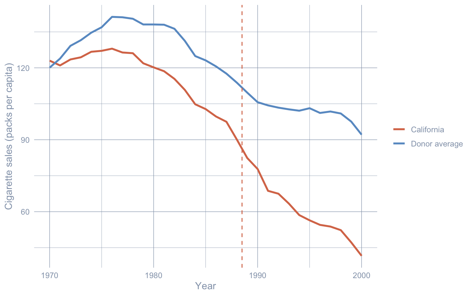
California already sat below the donor average in 1970 and the pre-period gap was widening, so a naive between-state comparison overstates the post-1988 effect. Chapter 4’s classical synthetic-control estimator picks a weighted donor blend that matches California’s pre-period level and slope — exactly to neutralise this pre-existing wedge.
1.10.5 Exercise 5 (stretch): Simulate a non-parallel-trends DGP
Generate a small synthetic 2-unit, 20-year panel where the treated unit follows a steeper downward trend than the control even in the absence of any policy. “Treat” the steeper-trending unit halfway through and apply the within-state naive pre/post estimator. Show with a plot and a one-line numerical summary that the naive estimator is biased even though there is no true treatment effect.
TipSolution
Code
set.seed(1)
sim <- tibble(
  year  = rep(2001:2020, times = 2),
  state = rep(c("treated", "control"), each = 20),
  trend = if_else(rep(c("treated", "control"), each = 20) == "treated",
                  -2, -0.5),
  noise = rnorm(40, sd = 1.5)
) |>
  group_by(state) |>
  mutate(y = 100 + trend * (year - 2001) + noise) |>
  ungroup() |>
  mutate(post = year >= 2011)

ggplot(sim, aes(year, y, color = state)) +
  geom_line(linewidth = 1) +
  geom_vline(xintercept = 2010.5, linetype = "dashed",
             color = "#d97757") +
  labs(x = "Year", y = "Outcome", color = NULL)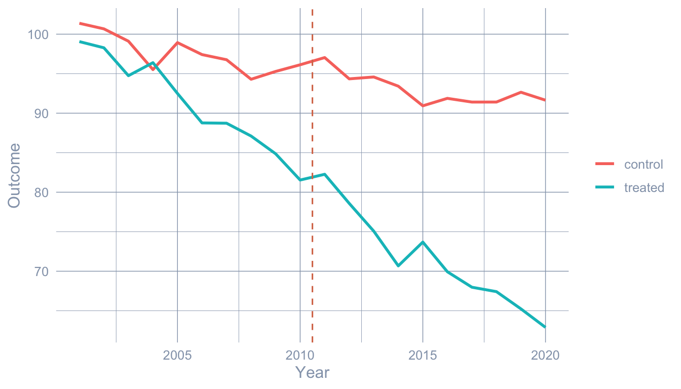
Code
sim |>
  filter(state == "treated") |>
  group_by(post) |>
  summarize(mean_y = mean(y), .groups = "drop") |>
  pivot_wider(names_from = post, values_from = mean_y,
              names_prefix = "post_") |>
  mutate(naive_att = post_TRUE - post_FALSE) |>
gt_pretty(decimals = 2)| post_FALSE | post_TRUE | naive_att |
|---|---|---|
| 91.2 | 71.37 | −19.83 |
There is no treatment effect in the data-generating process — post does not enter the equation for y — yet the within-state naive estimator returns a strongly negative “ATT” because the treated unit was already on a steeper downward trend before the cutoff. This is exactly the bias that ITS (ch. 2) addresses by modelling the pre-trend, and that synthetic control (ch. 4) addresses by matching the pre-period slope.