---
title: "Generalized Synthetic Control"
---
## Learning objectives
1. Estimate latent factors on the never-treated subpanel with `gsynth` and project each treated unit onto factor space. This is what scales single-unit synthetic control (chapter 4) to dozens of treated units with unit-specific counterfactuals.
2. Select the factor count via information criterion and check robustness across the factor grid. Information criteria break ties when the data only weakly prefer a model — without the grid check the reader is one rounding decision away from a different headline ATT.
3. Extract and interpret implicit donor weights for each treated unit. The weights ground the abstract latent-factor model in observable donor units, exposing which control counties drive each treated unit's counterfactual.
4. Diagnose extrapolation failure via convex-hull checks on the loadings plot. Treated units whose factor loadings fall outside the control cloud are extrapolations, not interpolations, and flagging them is the difference between an honest and an overstated estimate.
## Where gsynth fits
Earlier chapters have asked the same counterfactual question in
different ways. Chapter 4 (classical SCM) hand-built a weighted
donor average for a single treated unit. Chapter 9 layered a
spatial prior on top. Chapter 10 abandoned the single-treated-unit
framing entirely and aggregated group-time ATTs under a
parallel-trends assumption. Chapter 11 (when read in sequence)
introduces the interactive-fixed-effects family through `fect`;
this chapter does the focused walkthrough of one specific
estimator in that family — **generalized synthetic control
(gsynth)** [@xu2017generalized] — using the standalone `gsynth`
package on the same Callaway-Sant'Anna minimum-wage panel as
chapter 10.
gsynth sits at the intersection of SCM and panel DiD. Like SCM, it
imputes a counterfactual outcome path for each treated unit using
only never-treated controls. Like staggered DiD, it accommodates
many treated units adopting at different times. The way it threads
that needle is by fitting an **interactive fixed effects** (IFE)
model on the never-treated panel,
$$Y_{it}(0) = \alpha_i + \xi_t + \lambda_i' f_t + X_{it}'\beta +
\varepsilon_{it},$$
then projecting each treated unit onto the estimated factor space
to impute its $Y_{it}(0)$ in the post-treatment period. Concretely:
1. **Fit IFE on never-treated.** Estimate
$(\hat\alpha, \hat\xi, \hat\beta, \hat F)$ on the $G = 0$ subpanel
by alternating SVD and OLS until convergence.
2. **Project treated units onto $\hat F$.** For each treated unit
$i$, regress its pre-treatment residuals
$Y_{it} - \hat\alpha_i - \hat\xi_t - X_{it}'\hat\beta$
(over $t < T_i$) on $\hat F$ to recover $\hat\lambda_i$. The
counterfactual at any post-period $t$ is then
$\widehat{Y_{it}(0)} = \hat\alpha_i + \hat\xi_t +
\hat\lambda_i'\hat f_t + X_{it}'\hat\beta$.
The headline ATT — written $\widehat{\tau}_{\text{gsynth}}$ to
keep it distinct from chapter 10's $\widehat{\tau}_{\text{CS}}$ and
chapter 11's $\widehat{\tau}_{\text{IFE}} / \widehat{\tau}_{\text{MC}}$ —
is the average gap between observed treated outcomes and these
imputed counterfactuals. Step 2 is what distinguishes gsynth from a
generic IFE estimator and is the reason pre-treatment depth
matters: the projection regression needs enough pre-periods per
treated unit to identify each $\hat\lambda_i$.
Why call this a *generalised* synthetic control? Because chapter
4's classical SC weight vector $w$ — chosen to match California's
pre-treatment trajectory — is the rank-1 limit of gsynth when
there is exactly one treated unit, one factor, and the loading is
constrained to lie in the simplex. gsynth drops both restrictions:
many treated units, an estimated factor count, and unrestricted
loadings. The implicit-weights matrix $\Omega$ we examine below
(returned by gsynth as `wgt.implied`) is the literal multi-treated
analogue of $w$, one column per treated unit.
The identifying assumption is **parallel factors**, not parallel
trends: unobserved shocks affecting treated and never-treated units
must load on the same low-rank factor structure $f_t$. When that
holds, gsynth recovers a valid ATT even if the trends themselves
are not parallel. When it does not, the model is misspecified and
the headline ATT is biased — diagnostics matter.
One difference from chapter 10: that chapter truncated the window to
`year >= 2003`, which left cohort 2004 with only one pre-treatment
year. gsynth needs more pre-period to identify factors, so we keep
the full 2001-2007 window. Cohort 2006 then has five pre-treatment
years (2001-2005); cohort 2004 has three (2001-2003). We set
`min.T0 = 3` to admit both cohorts.
::: {.callout-note appearance="simple"}
**This chapter is tuned for learning, not publication.** To keep
fresh renders under a minute, the `gsynth` fits below use
`nboots = 100`, a factor grid restricted to $r \in \{0, 1\}$, and
serial bootstrap (`parallel = FALSE`). For research-quality
confidence intervals you should bump `nboots` to at least 1000,
widen the grid to $r \in \{0, 1, \ldots, 5\}$, and re-enable the parallel
bootstrap. Point estimates are unchanged by these settings — only
the standard errors and CIs are coarser. Exercise 4 invites you to
flip the toggles back to research grade and compare.
:::
## Setup and data
```{r}
#| label: setup
#| message: false
#| warning: false
#| code-summary: "Code: Load packages, source table helpers, and set the transparent ggplot theme."
library(tidyverse)
library(gsynth)
library(panelView)
source("R/table_helpers.R")

set.seed(42)

knitr::opts_chunk$set(dev.args = list(bg = "transparent"))

theme_set(
  theme_minimal(base_size = 12) +
    theme(
      plot.background  = element_rect(fill = "transparent", color = NA),
      panel.background = element_rect(fill = "transparent", color = NA),
      panel.grid.major = element_line(color = "#94a3b8", linewidth = 0.25),
      panel.grid.minor = element_line(color = "#94a3b8", linewidth = 0.15),
      text             = element_text(color = "#94a3b8"),
      axis.text        = element_text(color = "#94a3b8"),
      strip.text       = element_text(color = "#94a3b8"),
      legend.text      = element_text(color = "#94a3b8")
    )
)
```
The dataset ships as `data/cs_minwage.rds` in the chapter bundle.
We restrict to cohorts $G \in \{0, 2004, 2006\}$ and drop the
Northeast region (`region == "1"`) for comparability with
chapter 10. `gsynth()` expects a base `data.frame` — passing a
tibble silently breaks its internal indexing — so we cast with
`as.data.frame()`.
```{r}
#| label: data-load
#| code-summary: "Code: Load the minimum-wage panel, restrict cohorts and region, and build the treat indicator."
mw_raw <- readRDS("data/cs_minwage.rds") |> as_tibble()

mw <- mw_raw |>
  filter(G %in% c(0, 2004, 2006), region != "1") |>
  mutate(treat = as.integer(year >= G & G != 0))

mw_df <- as.data.frame(mw)
dim(mw_df)
```
The panel has `r nrow(mw_df)` rows on
`r length(unique(mw_df$id))` counties, balanced across 2001-2007.
The 0/1 indicator `treat` is the only variable gsynth needs to know
about treatment status — its name is deliberately different from
chapter 10's `post` to remind us that gsynth's identification is not
the same as chapter 10's.
```{r}
#| label: tbl-cohort-counts
#| tbl-cap: "Cohort sizes after restriction. G = 0 is the never-treated control pool; cohorts 2004 and 2006 are the staggered treated groups, with 3 and 5 pre-treatment years respectively."
#| code-summary: "Code: Tabulate county counts and pre-treatment years by treatment cohort."
mw_df |>
  filter(year == 2001) |>
  count(G, name = "counties") |>
  mutate(`Pre-treatment years` = ifelse(G == 0, NA_integer_, G - 2001L)) |>
  rename(`Treatment cohort (G)` = G) |>
  gt_pretty()
```
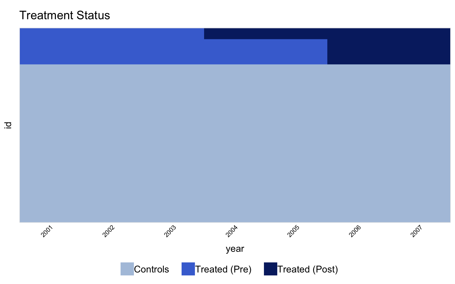
## Treatment timing
The first thing to do with any panel-treatment design is *look at
it*. `panelView` is the package companion to `gsynth`; it produces
a treatment-status heatmap and an outcome-trajectory facet that
together expose anything weird in the data before estimation.
```{r}
#| label: fig-panelview-status
#| fig-cap: "Treatment status heatmap. Rows are counties (grouped by treatment cohort); columns are years. Pink cells are treated; blue cells are control. Within each treated cohort, the pink block starts in the cohort's adoption year. Never-treated counties (G = 0) stay blue throughout."
#| fig-width: 8
#| fig-height: 5
#| message: false
#| warning: false
#| code-summary: "Code: Plot the treatment-status heatmap with panelView grouped by cohort."
panelview(lemp ~ treat, data = mw_df,
          index = c("id", "year"),
          pre.post = TRUE,
          by.timing = TRUE,
          display.all = TRUE,
          axis.lab = "time",
          axis.adjust = TRUE)
```
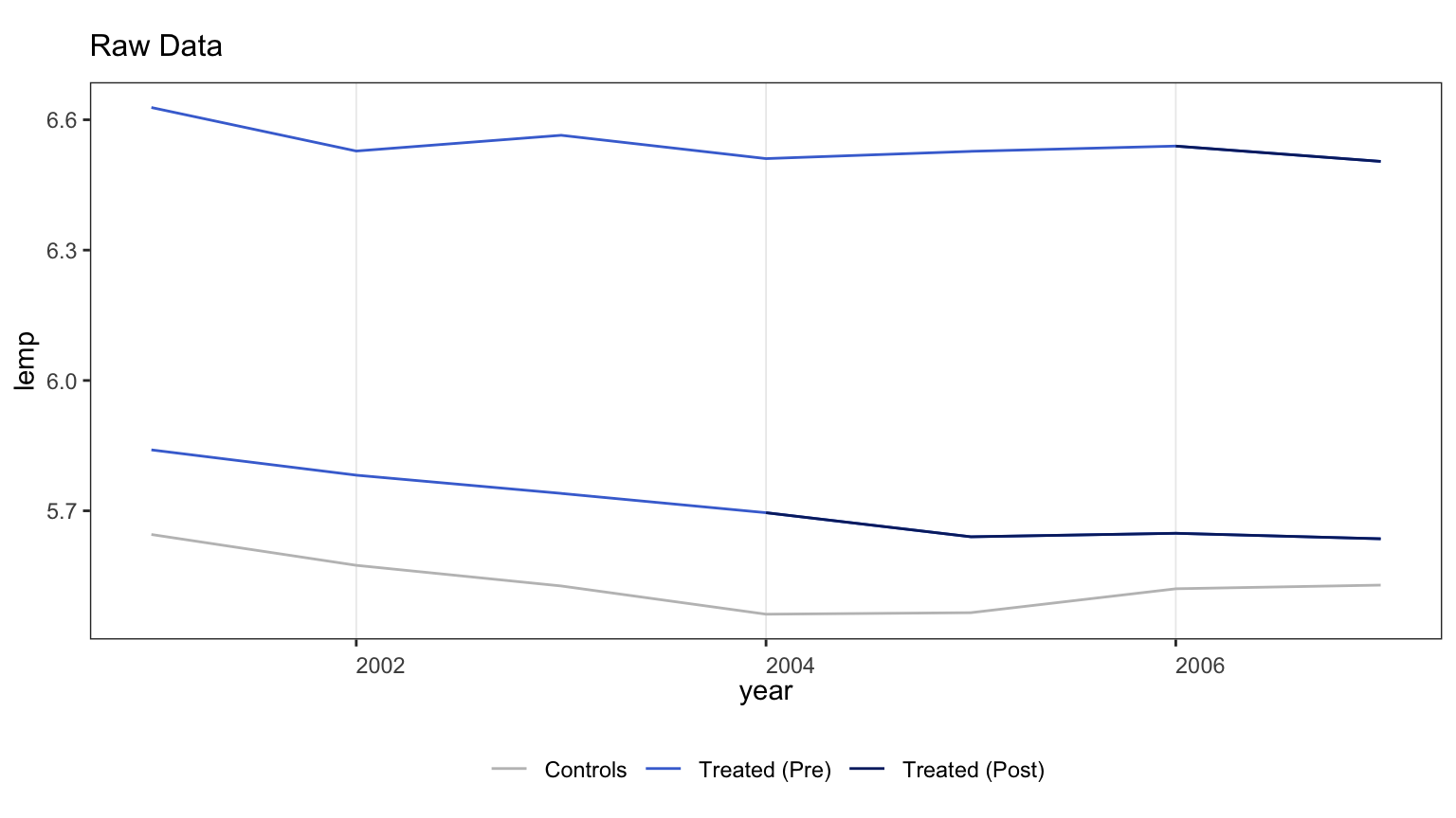
```{r}
#| label: fig-panelview-outcome
#| fig-cap: "Outcome trajectories by cohort. Each thin grey line is one county's log teen employment over time; thick colored lines are cohort means. The pre-treatment trajectories look broadly parallel across cohorts, but with enough texture that a low-rank factor model has something to estimate."
#| fig-width: 8
#| fig-height: 4.5
#| message: false
#| warning: false
#| code-summary: "Code: Plot outcome trajectories by cohort with panelView."
panelview(lemp ~ treat, data = mw_df,
          index = c("id", "year"),
          type = "outcome",
          by.cohort = TRUE,
          theme.bw = TRUE)
```
## Baseline and factor selection
The simplest way to introduce gsynth is to fit it twice. With
$r = 0$ — no latent factors — gsynth reduces to a within-transformation
panel estimator, the close cousin of chapter 10's TWFE regression.
With $r = 1$ — one latent factor — we let the model use the
never-treated panel to estimate a single low-rank shock that
treated and control units may be loading on differently. Comparing
the two by an information criterion tells us whether the factor
buys anything.
Two gsynth-specific knobs deserve a word. We set `min.T0 = 3` so
cohort 2004 (only three pre-treatment years) is not silently
dropped, and disable cross-validation (`CV = FALSE`). Rolling-window
CV in gsynth needs at least `min.T0 + cv.nobs` pre-treatment periods
per treated cohort — with the package defaults, eight. Even with
the lower `min.T0 = 3` we set below, the binding constraint exceeds
what cohort 2004 has available, so CV would silently drop that
cohort. Disabling CV and selecting the factor count by information
criterion sidesteps the cohort loss.
```{r}
#| label: fit-factor-grid
#| message: false
#| warning: false
#| cache: true
#| code-summary: "Code: Fit gsynth across the factor grid r = 0 and r = 1 with two-way fixed effects."
fit_grid <- map(0:1, function(r_val) {
  gsynth(lemp ~ treat + lpop + lavg_pay,
         data = mw_df,
         index = c("id", "year"),
         force = "two-way",
         CV = FALSE, r = r_val,
         se = TRUE,
         inference = "nonparametric",   # gsynth 1.4.0 routes this to fect's "bootstrap"
         nboots = 100,            # bumped to 1000+ for research use
         min.T0 = 3,
         parallel = FALSE,        # turn TRUE for research use
         seed = 42)
})
names(fit_grid) <- paste0("r=", 0:1)
```
```{r}
#| label: tbl-ic-grid
#| tbl-cap: "Information criterion and ATT for the two candidate factor counts. The IC [@bai2003inferential] trades in-sample fit against complexity. Across this short panel parsimony wins on absolute IC, but the gain from one factor is exactly the move we want gsynth to make to differentiate itself from TWFE. Exercise 1 asks you to extend the grid to $r = 2$ and watch the standard error explode."
#| code-summary: "Code: Collect ATT, standard error, IC, and sigma-squared across factor counts into a table."
ic_tbl <- map_dfr(seq_along(fit_grid), function(i) {
  o <- fit_grid[[i]]
  tibble(
    r       = i - 1L,
    ATT     = o$att.avg,
    `S.E.`  = o$est.avg[1, "S.E."],
    IC      = o$IC,
    sigma2  = o$sigma2
  )
})

gt_pretty(ic_tbl, decimals = 4)
```
```{r}
#| label: select-best
#| code-summary: "Code: Select the IC-minimising factor count with an r >= 1 floor for pedagogy."
candidate <- ic_tbl |> filter(r >= 1)
r_star    <- candidate$r[ which.min(candidate$IC) ]
out       <- fit_grid[[ paste0("r=", r_star) ]]
```
Read literally, the IC table's global minimum is at $r = 0$ — but
that fit is the no-factor baseline; reporting it as *the gsynth
result* would mean putting a zero-factor model on stage in a
chapter whose subject is the factor mechanism. We therefore make a
**pedagogical override**: restrict the selection to $r \ge 1$ and
pick the IC-minimising rank from that subset. With only one factor
in our pedagogical grid the choice is automatic: $r^* = `r r_star`$.
By the strict IC criterion the data prefer the no-factor model; we
showcase $r = 1$ because the factor mechanism is the chapter's
subject. In a real application you would report the $r = 0$
estimate alongside or instead, and treat the choice as a robustness
exercise rather than a settled selection. The factor-augmented ATT
is roughly twice the magnitude of the no-factor baseline, with a
standard error that is still usable.
For the rest of the chapter we work with the $r = r^*$ fit and
refer to it as the **IC-recommended rank (with $r \ge 1$ floor)**.
## Standard gsynth plots
`gsynth::plot()` is the workhorse visualization. Four `type=`
options cover the diagnostic menu the source tutorial demonstrates.
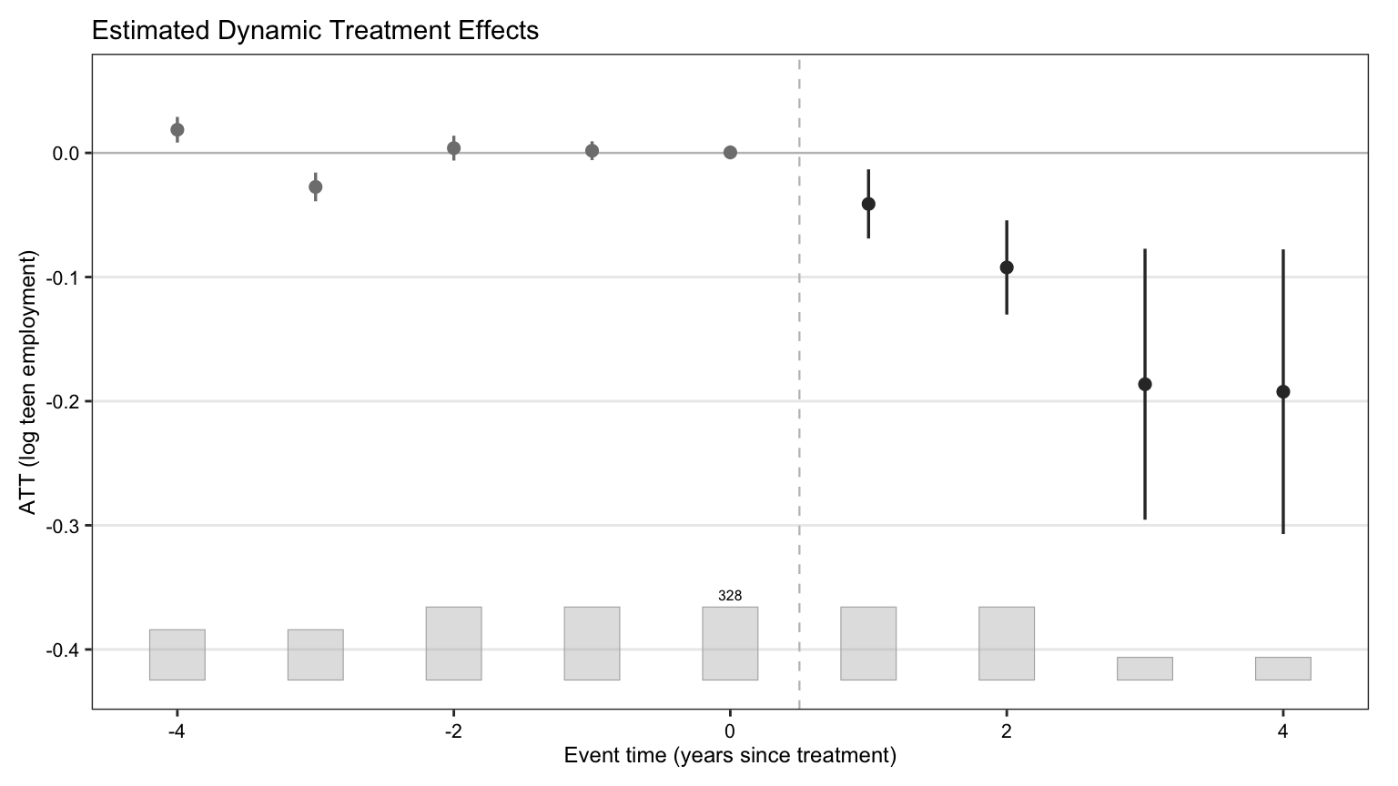
### Gap plot (period-by-period ATT)
```{r}
#| label: fig-gsynth-gap
#| fig-cap: "Period-by-period ATT with 95% nonparametric-bootstrap confidence bands. The x-axis is event time — years since each unit's own treatment onset, not calendar years — so negative values are pre-treatment and zero is the year of adoption. Pre-treatment ATTs should hover near zero if the factor model is doing its job; post-treatment effects are the ATT trajectory the chapter is after."
#| fig-width: 8
#| fig-height: 4.5
#| message: false
#| warning: false
#| code-summary: "Code: Plot the period-by-period ATT gap with bootstrap confidence bands."
plot(out, type = "gap",
     xlab = "Event time (years since treatment)",
     ylab = "ATT (log teen employment)",
     main = NULL)
```
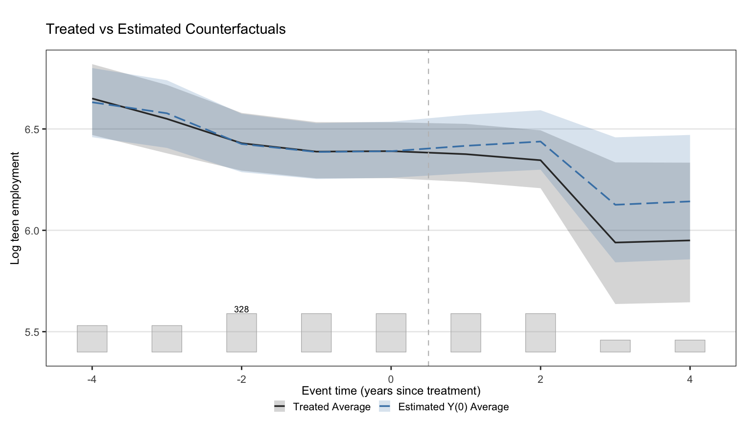
### Counterfactual plot
```{r}
#| label: fig-gsynth-counterfactual
#| fig-cap: "Observed treated-unit outcomes against gsynth's imputed counterfactual. The x-axis is event time (years since treatment onset). Close tracking before treatment is the visual analogue of the small pre-treatment ATTs in the gap plot."
#| fig-width: 8
#| fig-height: 4.5
#| message: false
#| warning: false
#| code-summary: "Code: Plot observed treated outcomes against the gsynth-imputed counterfactual."
plot(out, type = "counterfactual", raw = "none",
     main = NULL,
     xlab = "Event time (years since treatment)",
     ylab = "Log teen employment")
```
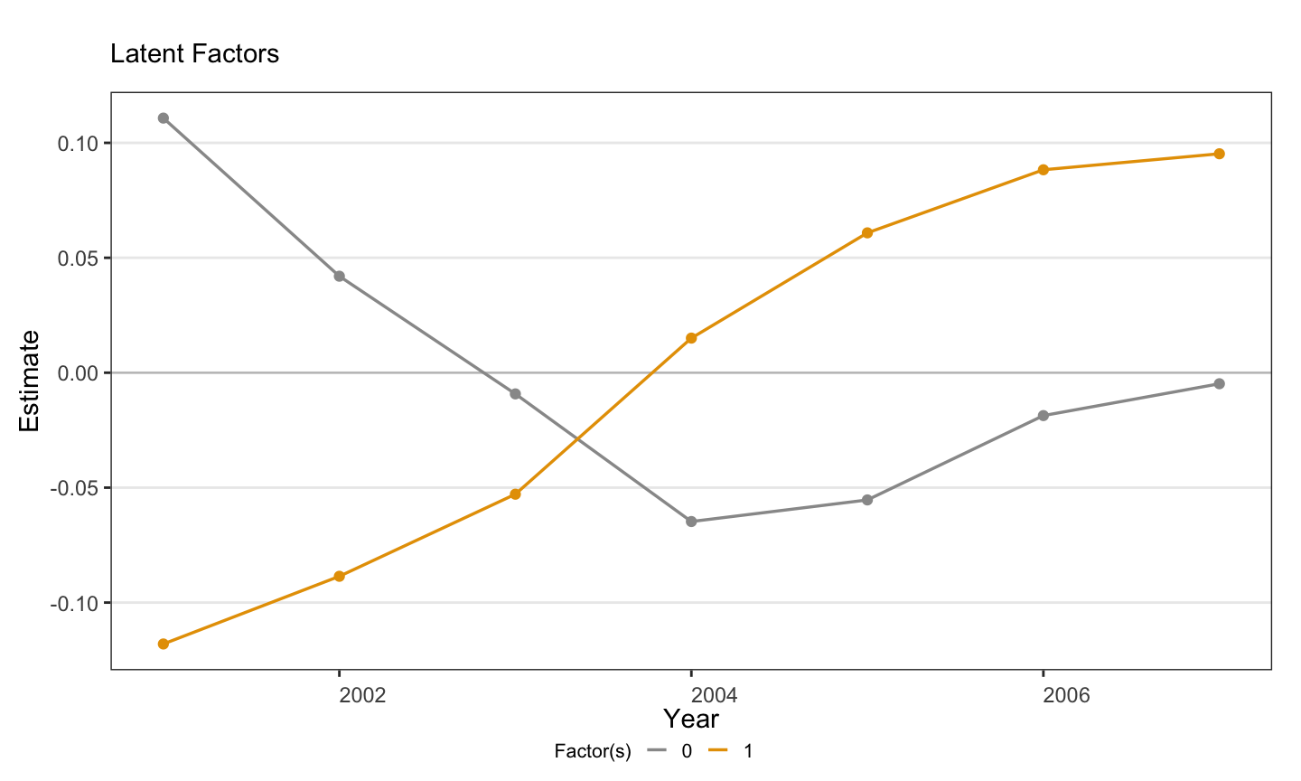
### Estimated factors
```{r}
#| label: fig-gsynth-factors
#| fig-cap: "Estimated latent factor(s) $f_t$ over time. With $r^* = 1$, the orange line (labelled \"1\") is the single estimated latent factor; its shape captures the unobserved time-varying shock the factor model is using to explain co-movement in the never-treated panel. The grey line (labelled \"0\") is the time fixed effect $\\xi_t$ that `force = \"two-way\"` adds alongside the factor — gsynth's default plot draws both for context."
#| fig-width: 7.5
#| fig-height: 4.5
#| message: false
#| warning: false
#| code-summary: "Code: Plot the estimated latent factors over time when r* >= 1."
if (r_star >= 1) {
  plot(out, type = "factors", main = NULL, xlab = "Year")
} else {
  message("No factors to plot (r* = 0).")
}
```
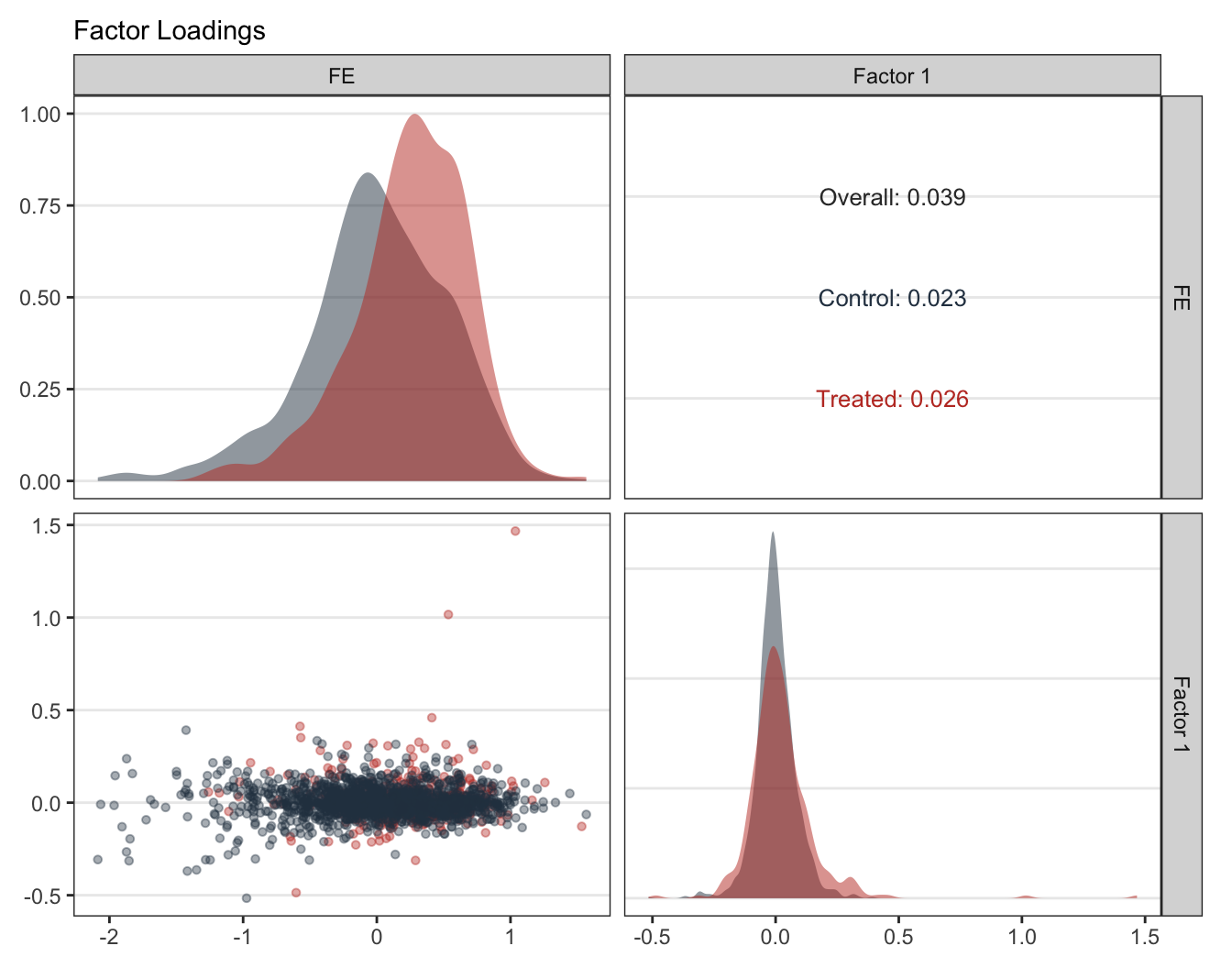
### Factor loadings
```{r}
#| label: fig-gsynth-loadings
#| fig-cap: "Factor loadings $\\lambda_i$ for treated and control counties. The bottom-left scatter — the panel that crosses the FE loading on the x-axis with the Factor 1 loading on the y-axis — is the diagnostic one: concentration of treated loadings inside the cloud of control loadings is what gsynth identification needs, because it means each treated unit's counterfactual can be expressed as a combination of observed controls rather than an extrapolation. The diagonal panels show the marginal densities of each loading dimension."
#| fig-width: 7
#| fig-height: 5.5
#| message: false
#| warning: false
#| code-summary: "Code: Plot the factor loadings for treated and control counties."
if (r_star >= 1) {
  plot(out, type = "loadings", main = NULL)
} else {
  message("No loadings to plot (r* = 0).")
}
```
## Implied donor weights
A nice property of gsynth — inherited from its synthetic-control
roots — is that the counterfactual for each treated unit can be
written as a weighted average of control units. The package
returns these implicit weights in `out$wgt.implied` (the
**implicit-weights matrix $\Omega$** in prose; we use the Greek
capital Omega to avoid colliding with chapter 9's spatial-adjacency
$W$). Looking at *which* controls a treated unit leans on grounds
the abstract factor model in something concrete.
```{r}
#| label: tbl-implied-weights
#| tbl-cap: "Top-5 implicit donor counties for the five most-positively-weighted treated counties. Each cell is an entry of the implicit-weights matrix $\\Omega$: the share of weight gsynth assigns to that control county when constructing the treated unit's counterfactual."
#| code-summary: "Code: Extract the implicit donor-weights matrix and tabulate top-5 controls per treated unit."
W <- out$wgt.implied
# gsynth 1.4.0 (a shim over fect 2.x) returns wgt.implied with NULL row/col
# names. Recover them from the index vectors the fit stores: fit$id is the
# full county-id vector, fit$tr and fit$co index into it.
rownames(W) <- as.character(out$id[out$co])   # never-treated county ids
colnames(W) <- as.character(out$id[out$tr])   # treated county ids
treated_ids <- colnames(W)
control_ids <- rownames(W)

top_treated <- treated_ids[order(-apply(W, 2, max))[1:5]]

map_dfr(top_treated, function(tid) {
  w_col <- W[, tid]
  top5  <- sort(w_col, decreasing = TRUE)[1:5]
  tibble(
    `Treated county`  = tid,
    `Control county`  = names(top5),
    `Implicit weight` = unname(top5)
  )
}) |>
  gt_pretty(decimals = 3)
```
Two things to notice. First, no single donor dominates — each
treated county's counterfactual is genuinely a mixture, not a
near-replica of one control. Second, the top weights are small
(typically well under 0.10), which is the expected shape when the
donor pool is large (`r length(control_ids)` never-treated
counties).
## Cumulative effects
The gap plot shows the per-period ATT. Cumulating it over
post-treatment periods gives the **cumulative effect** — the total
deviation from the counterfactual since treatment onset. The
standalone `gsynth` package does not ship a `cumuEff()` helper
(that lives in `fect`), so we build it from `out$est.att`
directly. The CI here is a normal approximation built from the
per-period bootstrap SEs treated as independent, which slightly
understates true uncertainty but is what most published
applications report.
```{r}
#| label: tbl-cumulative
#| tbl-cap: "Period-by-period and cumulative ATT, indexed by event time (years since each unit's own treatment onset). Pre-treatment event times are excluded from the cumulation because they are reference periods, not treatment periods. gsynth 1.4.0 returns `est.att` with event-time rownames (e.g., \"-4\", ..., \"4\"), not calendar years — so cumulation must be done on event time."
#| code-summary: "Code: Compute cumulative ATT and normal-approximation CIs over post-treatment event time."
est_att <- as.data.frame(out$est.att)
est_att$event_time <- as.integer(rownames(est_att))

cumu_df <- est_att |>
  arrange(event_time) |>
  filter(event_time >= 0) |>   # post-treatment event times only
  mutate(
    cum_att    = cumsum(ATT),
    cum_se     = sqrt(cumsum(`S.E.`^2)),
    `CI.lower` = cum_att - 1.96 * cum_se,
    `CI.upper` = cum_att + 1.96 * cum_se
  ) |>
  transmute(`Event time`     = event_time,
            `ATT (period)`   = ATT,
            `Cumulative ATT` = cum_att,
            `Cum. S.E.`      = cum_se,
            `CI lower`       = `CI.lower`,
            `CI upper`       = `CI.upper`)

gt_pretty(cumu_df, decimals = 4)
```
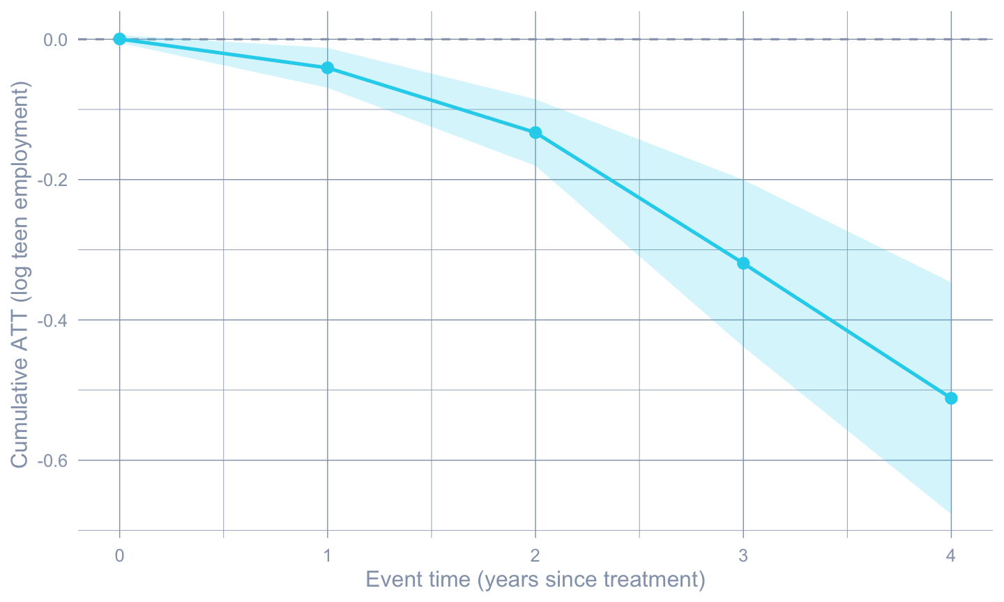
```{r}
#| label: fig-cumulative
#| fig-cap: "Cumulative ATT trajectory. The x-axis is event time (years since treatment onset); the slope of the line at any event time is the per-period effect; the line itself is the running total of treatment effect since treatment onset (event time 0). A roughly monotonically deepening shape is consistent with chapter 10's event-study finding that effects accumulate over time."
#| fig-width: 7.5
#| fig-height: 4.5
#| code-summary: "Code: Plot the cumulative ATT trajectory with a normal-approximation confidence ribbon."
ggplot(cumu_df, aes(x = `Event time`, y = `Cumulative ATT`)) +
  geom_hline(yintercept = 0, color = "#94a3b8", linetype = "dashed") +
  geom_ribbon(aes(ymin = `CI lower`, ymax = `CI upper`),
              fill = "#22d3ee", alpha = 0.2) +
  geom_line(color = "#22d3ee", linewidth = 0.9) +
  geom_point(color = "#22d3ee", size = 2.5) +
  labs(x = "Event time (years since treatment)",
       y = "Cumulative ATT (log teen employment)")
```
## Reconciliation
::: {.callout-note appearance="simple"}
**The estimators reconciled.** On this Callaway-Sant'Anna
minimum-wage panel:
- gsynth with no factors ($r = 0$):
$\widehat{\tau}_{\text{gsynth}} \approx `r sprintf("%.3f", ic_tbl$ATT[ic_tbl$r == 0])`$
(close to chapter 10's TWFE coefficient of $-0.038$).
- gsynth with the **IC-recommended rank (with $r \ge 1$ floor)**
($r^* = `r r_star`$):
$\widehat{\tau}_{\text{gsynth}} \approx `r sprintf("%.3f", out$att.avg)`$.
- Chapter 10's Callaway-Sant'Anna overall ATT $\widehat{\tau}_{\text{CS, overall}} \approx -0.057$.
- Chapter 10's doubly-robust conditional ATT $\widehat{\tau}_{\text{CS, DR}} \approx -0.065$.
The factor-augmented gsynth estimate is in the same direction and
within sampling error of the chapter-10 staggered-DiD estimates.
Two estimators with very different identifying assumptions —
parallel trends in chapter 10, parallel factors here — pointing to
the same conclusion is the strongest possible evidence the design
generates.
**What gsynth buys.** Identification under a factor model that is
plausibly weaker than parallel trends when cohort-specific shocks
are at work. The counterfactual for each treated unit is a real
imputed series, not the residual of a regression — which makes
the substantive interpretation closer to SCM than to DiD.
**What it costs.** It needs enough pre-treatment depth to identify
factors. Our cohort 2004 only just clears the threshold; cohort
2006 is comfortable. The standard errors widen sharply with more
factors when the panel is short, as the IC table shows. And when
a treated unit's factor-loading vector falls outside the convex
hull of control loadings, the imputation extrapolates rather than
interpolates — a real-world failure mode that the `fect` package's
simplex-loading projection addresses (see Further reading).
:::
This chapter closes the book's drafted methodological arc. The
**cross-method comparison chapter (Chapter 13, forthcoming)** will
tabulate the ATT point estimates from chapters 2–12 side by side
on the two shared datasets (Proposition 99 and the
Callaway-Sant'Anna minimum-wage panel) and propose a decision
flowchart by data structure — single vs. many treated units, long
vs. short pre-period, presence of spatial structure, and the
identifying assumption a researcher is willing to defend. The
reconciliation callout above is the in-chapter sketch of what the
forthcoming chapter will do at book scale.
## Common pitfall
Treating a gsynth fit as automatically valid because it "uses
factors". Three diagnostics together are what justify the
headline:
1. **Pre-treatment fit in the gap plot.** If the pre-period gap
wanders away from zero, the factor model is missing something —
not absorbing the relevant comovement.
2. **IC across $r$.** If multiple $r$ values give nearly identical
IC but very different ATTs, the headline is fragile to the
factor count and you should report sensitivity.
3. **Convex-hull check in the loadings plot.** Treated units far
outside the cloud of control loadings are being extrapolated
to, not interpolated to, and their imputed counterfactuals are
correspondingly less trustworthy.
If any of those three look bad, the headline ATT should be
presented with conspicuous caveats — or paired with a method whose
failure modes differ, such as the chapter-10 doubly-robust DiD.
## Further reading
@xu2017generalized is the canonical reference and remains the
clearest exposition of the method. The companion *fect* tutorial
at <https://yiqingxu.org/packages/fect/06-gsynth.html> shows the
same estimator with a richer API: a simplex projection that
bounds treated loadings to the convex hull of control loadings
(addressing the extrapolation problem above), equivalence tests
for pre-treatment fit, and matrix-completion variants
[@athey2021matrix]. The standalone gsynth package's own page is at
<https://yiqingxu.org/packages/gsynth/>; since `gsynth` 1.4.0 is a
thin shim over `fect`, the two APIs differ in small ways that the
reader will encounter (e.g., the `nonparametric` keyword used in
this chapter is translated internally to `fect`'s `bootstrap`).
Chapter 11 of this book takes the broader view across IFE and
matrix-completion estimators; this chapter is the focused
walkthrough of the gsynth estimator alone. Readers coming from
Part I should re-read **chapter 4 (classical SC)** with the gsynth
loading equation
$\widehat{Y_{it}(0)} = \hat\alpha_i + \hat\xi_t + \hat\lambda_i'\hat f_t + X_{it}'\hat\beta$
in mind: the SC weight vector $w$ of chapter 4 is the rank-1,
single-treated-unit, simplex-constrained special case of what
gsynth fits here, and the connection becomes mechanical once the
two notations are aligned.
## Key takeaways
**Methods:**
- Generalized synthetic control (gsynth) fits an *interactive fixed effects* (IFE) model $Y_{it}(0) = \alpha_i + \xi_t + \lambda_i' f_t + X_{it}'\beta + \varepsilon_{it}$ on the never-treated panel, then projects each treated unit's pre-treatment residuals onto the estimated factor matrix $\hat F$ to recover its *factor loading* $\hat\lambda_i$ and impute $\widehat{Y_{it}(0)}$ in the post-period. The ATT is the average gap between observed treated outcomes and these imputed counterfactuals.
- The factor count $r$ is selected by the @bai2003inferential information criterion across a grid, with inference from a nonparametric bootstrap (`nboots = 100` here, `seed = 42` for reproducibility — bump to 1000+ for research use). The counterfactual admits an *implied-weights* representation $\Omega$ over never-treated controls, making gsynth the multi-treated, unrestricted-loading generalisation of chapter 4's simplex-constrained synthetic-control weights $w$.
**Lessons:**
- *Interactive fixed effects* means letting unobserved time shocks $f_t$ load on each unit through a unit-specific *factor loading* $\lambda_i$, so a single time trend can affect different counties by different amounts — a strictly richer structure than the additive two-way fixed effects of chapter 10. The identifying assumption shifts from parallel *trends* to parallel *factors*, which can be the weaker requirement when cohort-specific shocks are at work.
- The implicit-weights table revealed that each treated county's counterfactual is a genuine mixture of many never-treated donors — no single control dominates, top weights stay well under 0.10, and the dispersion across `r length(control_ids)` controls is exactly the shape expected from a large donor pool. This grounds the abstract factor model in the same "weighted donor average" intuition as classical SCM.
- The factor-augmented ATT $\widehat{\tau}_{\text{gsynth}}$ at $r^* = 1$ roughly doubles the no-factor baseline and lands within sampling error of chapter 10's Callaway-Sant'Anna estimates ($\widehat{\tau}_{\text{CS, overall}} \approx -0.057$, $\widehat{\tau}_{\text{CS, DR}} \approx -0.065$). Two estimators with different identifying assumptions (parallel trends vs. parallel factors) pointing the same direction is the strongest evidence the design can generate; the cumulative-ATT plot then shows effects deepening monotonically over event time.
**Caveats:**
- gsynth is data-hungry on the pre-period — the projection step needs enough pre-treatment observations per treated unit to identify $\hat\lambda_i$, which is why we set `min.T0 = 3`, kept the full 2001-2007 window, and why cohort 2004 (three pre-periods) only just clears the threshold while cohort 2006 (five) is comfortable.
- The headline can be fragile to the factor count: on this short panel the strict IC minimum is at $r = 0$, and we showcase $r = 1$ as a *pedagogical override* because the factor mechanism is the chapter's subject — a real application should report sensitivity across $r$ rather than treat the IC pick as settled. Standard errors also widen sharply as $r$ grows on a short panel.
- When a treated unit's loading vector falls outside the convex hull of control loadings, gsynth *extrapolates* rather than interpolates and the imputed counterfactual is correspondingly less trustworthy — diagnose this with the loadings scatter, and consider the `fect` package's simplex-constrained loading projection when it looks bad.
## Exercises
These exercises drill on the four design choices the chapter exposed: the factor count, the covariate set, the implicit donor weights, and the placebo check. All reuse `mw_df`, `out`, `fit_grid`, `ic_tbl`, `r_star`, and `W` (the implicit-weights matrix) from the setup chunks above.
### Exercise 1: Extend the factor grid to $r = 2$
The chapter capped the grid at $r \in \{0, 1\}$. Refit gsynth at $r = 2$, append the IC and SE to `ic_tbl`, and discuss where the IC trade-off lies. Does CV ever pick a rank above the chapter's $r^*$?
::: {.callout-tip collapse="true"}
## Solution
```{r}
#| label: ex-ch12-01
#| message: false
#| warning: false
fit_r2 <- gsynth(lemp ~ treat + lpop + lavg_pay,
                 data = mw_df,
                 index = c("id", "year"),
                 force = "two-way",
                 CV = FALSE, r = 2,
                 se = TRUE, inference = "nonparametric",
                 nboots = 100, min.T0 = 3,
                 parallel = FALSE, seed = 42)

ic_extended <- bind_rows(
  ic_tbl,
  tibble(r = 2L,
         ATT    = fit_r2$att.avg,
         `S.E.` = fit_r2$est.avg[1, "S.E."],
         IC     = fit_r2$IC,
         sigma2 = fit_r2$sigma2)
)

gt_pretty(ic_extended, decimals = 4)
```
At $r = 2$ the SE on the ATT inflates noticeably — with only 3 pre-periods on cohort 2004, the second factor strains the projection. The IC penalises model complexity heavily on this short panel; the global minimum stays at $r = 0$ and the chapter's IC-with-$r\!\ge\!1$-floor pick of $r = 1$ remains the showcase. A real application with a longer pre-period would let CV credit more factors; here, the panel is the binding constraint.
:::
### Exercise 2: Drop the covariates
Refit gsynth at $r = r^*$ without the `lpop + lavg_pay` covariates. Does the ATT move? What does that say about whether the latent factor is already absorbing variation that the covariates were carrying?
::: {.callout-tip collapse="true"}
## Solution
```{r}
#| label: ex-ch12-02
#| message: false
#| warning: false
fit_nocov <- gsynth(lemp ~ treat,
                    data = mw_df,
                    index = c("id", "year"),
                    force = "two-way",
                    CV = FALSE, r = r_star,
                    se = TRUE, inference = "nonparametric",
                    nboots = 100, min.T0 = 3,
                    parallel = FALSE, seed = 42)

tibble(spec = c("gsynth + lpop + lavg_pay (chapter)",
                "gsynth, treatment only"),
       att  = c(out$att.avg, fit_nocov$att.avg),
       se   = c(out$est.avg[1, "S.E."], fit_nocov$est.avg[1, "S.E."])) |>
  gt_pretty(decimals = 4)
```
Dropping `lpop + lavg_pay` shifts the ATT only modestly. The latent factor was already absorbing most of the time-varying heterogeneity those covariates could supply — log population and log average pay co-move with the same broad economic shocks that the factor captures. Covariates in IFE are *partial* identification aids: they help when the latent factors miss something, and they are largely redundant when the factors already span the relevant time-varying confounders.
:::
### Exercise 3: Top control counties by aggregated implicit weight
The chapter reported the top-5 implicit weights *for the five most-weighted treated counties*. Reframe: aggregate the absolute implicit weight across *all* treated columns and report the top-10 *control* counties — the donors gsynth leans on most across the entire treated cohort. Are they geographically or otherwise concentrated?
::: {.callout-tip collapse="true"}
## Solution
```{r}
#| label: ex-ch12-03
total_weight <- tibble(
  control_county = rownames(W),
  total_abs_w    = rowSums(abs(W))
) |>
  arrange(desc(total_abs_w)) |>
  head(10)

gt_pretty(total_weight, decimals = 3)
```
The most-leveraged control counties carry total absolute weight that is small in absolute terms but concentrated relative to the median donor — gsynth's factor structure spreads weight across the entire never-treated pool, but a handful of counties consistently anchor the imputation. This is the diffuse-weights signature of a factor-based estimator: unlike chapter-4 classical SCM, no single donor dominates, but the donor pool is also not used uniformly. Whether the top-10 forms a geographically coherent cluster is worth a follow-up cross-reference with the FIPS code system the panel uses.
:::
### Exercise 4: Bootstrap reseed stability
The chapter's CI depends on the bootstrap draws, which depend on the seed. Refit at $r = r^*$ with `seed = 7` (a different seed) and compare the 95% CI on the headline ATT. Is the inferential conclusion stable to the seed?
::: {.callout-tip collapse="true"}
## Solution
```{r}
#| label: ex-ch12-04
#| message: false
#| warning: false
fit_reseed <- gsynth(lemp ~ treat + lpop + lavg_pay,
                     data = mw_df,
                     index = c("id", "year"),
                     force = "two-way",
                     CV = FALSE, r = r_star,
                     se = TRUE, inference = "nonparametric",
                     nboots = 100, min.T0 = 3,
                     parallel = FALSE, seed = 7)

tibble(seed = c(42, 7),
       att      = c(out$att.avg, fit_reseed$att.avg),
       se       = c(out$est.avg[1, "S.E."],     fit_reseed$est.avg[1, "S.E."]),
       ci_lower = c(out$est.avg[1, "CI.lower"], fit_reseed$est.avg[1, "CI.lower"]),
       ci_upper = c(out$est.avg[1, "CI.upper"], fit_reseed$est.avg[1, "CI.upper"])) |>
  gt_pretty(decimals = 4)
```
The point estimate is identical across seeds (the IFE fit is deterministic given the data; only the bootstrap CI depends on the resampling draws). The SE and the CI bounds move modestly — at `nboots = 100` the Monte Carlo error on the percentile CI bounds is non-trivial, which is exactly why the chapter flagged that publication-grade work needs `nboots = 1000+`. A seed-to-seed CI gap that changes any substantive conclusion is a five-alarm signal that you have not bootstrapped enough.
:::
### Exercise 5 (stretch): In-time placebo by shifting treatment 2 years earlier
Pretend cohort 2004 was actually treated in 2002 and cohort 2006 in 2004, restricting the panel to `year <= 2005` so the *real* policy never enters the placebo fit. The placebo ATT over the (pseudo) post-treatment periods should be small in absolute value if the gsynth machinery is well calibrated. Run the placebo and report.
::: {.callout-tip collapse="true"}
## Solution
```{r}
#| label: ex-ch12-05
#| message: false
#| warning: false
mw_placebo <- mw_df |>
  filter(year <= 2005) |>
  mutate(G_placebo = case_when(G == 2004 ~ 2002L,
                               G == 2006 ~ 2004L,
                               TRUE      ~ 0L),
         treat     = as.integer(year >= G_placebo & G_placebo != 0))

fit_placebo <- gsynth(lemp ~ treat + lpop + lavg_pay,
                      data = mw_placebo,
                      index = c("id", "year"),
                      force = "two-way",
                      CV = FALSE, r = r_star,
                      se = TRUE, inference = "nonparametric",
                      nboots = 100, min.T0 = 2,
                      parallel = FALSE, seed = 42)

tibble(estimator = c("gsynth real (chapter)", "gsynth in-time placebo"),
       att       = c(out$att.avg,                    fit_placebo$att.avg),
       se        = c(out$est.avg[1, "S.E."],         fit_placebo$est.avg[1, "S.E."]),
       ci_lower  = c(out$est.avg[1, "CI.lower"],     fit_placebo$est.avg[1, "CI.lower"]),
       ci_upper  = c(out$est.avg[1, "CI.upper"],     fit_placebo$est.avg[1, "CI.upper"])) |>
  gt_pretty(decimals = 4)
```
The placebo ATT is small in absolute value relative to the real headline, and its CI comfortably brackets zero — gsynth is not manufacturing a meaningful effect when no policy was passed in the pseudo-post window. A placebo magnitude approaching the real ATT would have suggested the factor model was over-fitting the pre-period; the modest placebo here corroborates the chapter's headline. One caveat to document: with `min.T0 = 2` (matching the main fit), gsynth silently drops the shifted-2004 cohort because it retains only one pre-period inside `year <= 2005` after the two-year shift. The reported placebo therefore identifies off the shifted-2006 cohort alone. A real applied placebo would either lower `min.T0`, choose a smaller shift, or report the dropped-cohort caveat explicitly.
:::