---
title: "Synthetic Control with Prediction Intervals"
---
## Learning objectives
1. Fit synthetic-control weights under four regularization regimes (simplex, lasso, ridge, OLS) from `scpi`'s single API. Running all four at once is how the reader checks whether their headline estimate is a constraint artifact rather than a data finding.
2. Construct finite-sample prediction intervals by decomposing SC error into in-sample weight uncertainty and out-of-sample shocks. These are the first SC intervals in the book with proven frequentist coverage, and replacing chapter 4's permutation *p*-value with a coverage statement is what makes the method publishable in econometrics venues.
3. Set Bonferroni-adjusted alpha splits (`u.alpha`, `e.alpha`) so a stated joint coverage level is the actual joint coverage level. Without the split the union bound is violated and the interval's nominal coverage is unachieved, even though the "95% PI" label still appears on the plot.
4. Sweep confidence levels (80/90/95/99%) and report at which level the post-period outcome reliably exits the band. The sweep is the natural way to quantify evidence strength when a single conventional level is arbitrary.
## Why a third synthetic-control chapter?
Chapter 4 fit the classical synthetic-control estimator with `tidysynth`: donor weights live on the simplex, and the inference story is the Fisher-exact placebo permutation test. Chapter 5 added a ridge outcome-model bias correction; chapter 6 ran DiD on a doubly de-meaned panel; chapter 7 produced posterior **credible** intervals (CrI) from a structural Bayesian time-series model — a probability statement about the parameter, conditional on the prior.
What is still missing is a **frequentist** uncertainty story for the synthetic-control estimator itself. The Fisher p-value from chapter 4 is a rank statistic — it tells us California is unusual relative to the donor pool, but it does not give us a *prediction interval* with finite-sample coverage guarantees. The `scpi` package of @cattaneo2021prediction and @cattaneo2025scpi closes that gap. It decomposes synthetic-control forecast error into two components — in-sample weight uncertainty and out-of-sample post-treatment shocks — and constructs a **prediction interval (PI)** $\widehat{\text{PI}}_{1t}$ that covers the synthetic counterfactual $\widehat{Y_{1t}(0)}$ with stated finite-sample frequentist coverage. The CrI of chapter 7 and the PI of this chapter answer different questions: the CrI is a posterior over the effect given a prior; the PI is a sampling-distribution band around the counterfactual prediction.
`scpi` also generalises the weight-estimation step. The same API fits the **simplex** (classical Abadie–Diamond–Hainmueller), **lasso**, **ridge**, and **OLS** constraints from a single function call, so we can ask a sharper question than chapter 4 could: *is the headline ATT a consequence of the simplex constraint, or does it survive every reasonable choice of donor regularisation?* We will write the resulting point estimate as $\widehat{\tau}_{\text{scpi}}$ — adding a constraint subscript such as $\widehat{\tau}_{\text{scpi-simplex}}$ when we need to distinguish the four constraint families — to keep it distinct from chapter 4's $\widehat{\tau}_{\text{SCM}}$, chapter 5's $\widehat{\tau}_{\text{ASCM}}$, chapter 6's $\widehat{\tau}_{\text{SDID}}$, and chapter 7's $\widehat{\tau}_{\text{BSTS}}$.
## The framework
Let $Y_{1t}$ be the treated unit's outcome at time $t$, and $Y_{0t}$ the $J$-vector of donor outcomes. The synthetic-control predictor is
$$\widehat{Y_{1t}(0)} \,=\, \sum_{j} \widehat{w}_j \, Y_{jt} \,=\, \widehat{w}^\top Y_{0t},$$
with weights $\widehat{w} = (\widehat{w}_1, \ldots, \widehat{w}_J)$ chosen on the pre-period under one of four constraint sets: simplex ($\widehat{w}_j \ge 0$ and $\sum_j \widehat{w}_j = 1$), lasso ($\|\widehat{w}\|_1 \le Q$), ridge ($\|\widehat{w}\|_2 \le Q$), or OLS (unconstrained). The per-period treatment effect is $\widehat{\tau}_t = Y_{1t} - \widehat{Y_{1t}(0)}$, and the ATT estimator is its post-period average $\widehat{\tau}_{\text{scpi}} = T_{\text{post}}^{-1} \sum_{t > t^*} \widehat{\tau}_t$.
The error in estimating the *counterfactual* at any post-period $t$ decomposes as
$$Y_{1t}(0) \;-\; \widehat{Y_{1t}(0)} \;=\; \underbrace{(w^* - \widehat{w})^\top Y_{0t}}_{\text{in-sample error}} \;+\; \underbrace{e_t}_{\text{out-of-sample error}}.$$
The first term, the in-sample component, comes from estimating the donor weights on a finite pre-period — sampling variability propagates into the counterfactual. The second term, $e_t$, captures post-treatment shocks and structural drift that the pre-period cannot anticipate; it grows with the forecast horizon. The placebo test in chapter 4 sidesteps this decomposition entirely — it ranks California against permuted-treatment states without modelling either error source — and so produces a $p$-value rather than an interval. `scpi` quantifies the two error sources separately and reports a prediction interval $\widehat{\text{PI}}_{1t} = [\widehat{Y_{1t}(0)} - L_t,\, \widehat{Y_{1t}(0)} + U_t]$ around the *counterfactual prediction*, with stated finite-sample coverage.
In chapter 4's notation we would write the same predictor with the V-weighted predictor objective augmented by auxiliary covariates. This chapter omits the predictor matrix $X$ entirely (see Setup) and so works directly with donor outcomes $Y_{0t}$. A parallel frequentist-coverage literature builds prediction intervals via *conformal inference* (Chernozhukov, Wüthrich & Zhu 2021, *JASA*), which trades the parametric in-sample / out-of-sample decomposition for distribution-free quantile guarantees; see Further reading.
The substantive interpretation matters and is the first pitfall of the chapter: the prediction interval $\widehat{\text{PI}}_{1t}$ bounds the *synthetic counterfactual* $\widehat{Y_{1t}(0)}$, not the treatment effect $\widehat{\tau}_t$ and not the observed series. Because $Y_{1t}$ is observed (not random conditional on the pre-period), the band can be flipped about the observed series to produce a band for $\widehat{\tau}_t$ — exercise 3 does this — but the primary inferential statement is geometric: the treatment effect is "statistically distinct from forecasting noise" when observed California sits *outside* $\widehat{\text{PI}}_{1t}$, most commonly when it falls *below* the lower bound of the band built around synthetic California.
## Setup and data
```{r}
#| label: setup
#| message: false
#| warning: false
#| code-summary: "Code: Load packages, source table helpers, set seed, and configure ggplot theme."
library(tidyverse)
library(scpi)
source("R/table_helpers.R")

set.seed(42)

knitr::opts_chunk$set(dev.args = list(bg = "transparent"))

theme_set(
  theme_minimal(base_size = 12) +
    theme(
      plot.background  = element_rect(fill = "transparent", color = NA),
      panel.background = element_rect(fill = "transparent", color = NA),
      panel.grid.major = element_line(color = "#94a3b8", linewidth = 0.25),
      panel.grid.minor = element_line(color = "#94a3b8", linewidth = 0.15),
      text             = element_text(color = "#94a3b8"),
      axis.text        = element_text(color = "#94a3b8")
    )
)
```
The chapter reuses the Proposition 99 dataset that powered chapters 2–4 and 6–7: 39 US states, 1970–2000, with `cigsale` as the outcome (per-capita cigarette sales in packs). `scpi`'s `scdata()` wants the unit identifier as character — coerce the factor before handing it off. We use only the outcome series for matching (matching the configuration of the `scpi_pkg` Python illustration in @cattaneo2025scpi); the auxiliary covariates `lnincome`, `beer`, and `age15to24` carry many NAs in the early pre-period and would force row deletions that bias the donor pool.
This is an intentional departure from chapter 4, which used `lnincome`, `beer`, and `age15to24` as auxiliary predictors via `tidysynth::generate_predictor()`. The covariate-rich match in chapter 4 produces a tighter pre-period fit and a more negative simplex ATT — $\widehat{\tau}_{\text{SCM}} \approx -18.85$; outcome-only matching here is more conservative, is more honest about the missing-data structure, and lands at a smaller $\widehat{\tau}_{\text{scpi-simplex}}$ (≈ $-11$, see below). We return to this comparison in the Recap.
```{r}
#| label: data-load
#| code-summary: "Code: Load the Proposition 99 panel and build the donor state list."
prop99 <- read_rds("data/proposition99.rds") |>
  as_tibble() |>
  mutate(state = as.character(state))

donors <- setdiff(sort(unique(prop99$state)), "California")
```
## Preparing the data for `scpi`
`scdata()` reshapes the long panel into the matrices `A` (treated pre-outcome), `B` (donor pre-outcomes), `P` (donor post-outcomes), and `Y.pre` / `Y.post` used downstream by `scest()` and `scpi()`. The two flags worth understanding for cigarette sales are `cointegrated.data = TRUE` (the long-run-variance adjustment for the I(1)-looking `cigsale` series, which only affects the inference step) and `constant = TRUE` (a single intercept across features — keeping the chapter close to the JSS illustration).
```{r}
#| label: scdata-prep
#| message: false
#| warning: false
#| code-summary: "Code: Reshape the panel into scpi matrices via scdata() for California vs donor states."
data_prep <- scdata(
  df               = prop99,
  id.var           = "state",
  time.var         = "year",
  outcome.var      = "cigsale",
  period.pre       = 1970:1988,
  period.post      = 1989:2000,
  unit.tr          = "California",
  unit.co          = donors,
  cointegrated.data = TRUE,
  constant         = TRUE
)
```
`data_prep` carries 19 pre-period years and 12 post-period years, with $J = 38$ donor states ready to be combined.
## Point estimation across four weight constraints
`scest()` is the deterministic counterpart to `scpi()`: it solves for the donor weights under a chosen constraint and returns the synthetic counterfactual, but no prediction interval. Running it four times with `w.constr = list(name = ...)` swaps the constraint and leaves everything else identical, so any difference in the fitted weights is attributable to the regulariser alone.
```{r}
#| label: scest-four
#| message: false
#| warning: false
#| code-summary: "Code: Fit scest point estimates under simplex, lasso, ridge, and OLS constraints."
constraints <- c("simplex", "lasso", "ridge", "ols")

scest_fits <- map(constraints, \(name) {
  scest(data_prep, w.constr = list(name = name))
}) |>
  set_names(constraints)
```
The four constraint sets correspond to four classical optimisation problems on the weight vector $\widehat{w}$: simplex ($\widehat{w}_j \ge 0$, $\sum_j \widehat{w}_j = 1$), lasso ($\|\widehat{w}\|_1 \le Q$ with $Q$ a tuning parameter, default $Q = 1$ in `scpi`, no sign restriction), ridge ($\|\widehat{w}\|_2 \le Q$ with $Q$ chosen from the data as $(J + K)\widehat{\sigma}_u^2 / \|\widehat{w}_{\rm OLS}\|_2^2$), and OLS (unconstrained least squares). Each problem encodes a different prior about how donor information should flow into the synthetic.
## Donor weights side-by-side
```{r}
#| label: tbl-weights-side-by-side
#| tbl-cap: "Donor weights from each of the four scpi weight-constraint families, for the 12 donors with largest maximum absolute weight across the four constraints."
#| code-summary: "Code: Tabulate the top-12 donor weights side-by-side across the four constraints."
weight_long <- map_dfr(constraints, \(name) {
  w <- scest_fits[[name]]$est.results$w
  tibble(
    constraint = name,
    state      = sub("^.*\\.", "", names(w)),
    weight     = as.numeric(w)
  )
})

weight_wide <- weight_long |>
  pivot_wider(names_from = constraint, values_from = weight, values_fill = 0)

weight_wide |>
  mutate(rank_score = pmax(abs(simplex), abs(lasso), abs(ridge), abs(ols))) |>
  arrange(desc(rank_score)) |>
  head(12) |>
  select(state, simplex, lasso, ridge, ols) |>
  gt_pretty(decimals = 3) |>
  gt::cols_label(
    state = "Donor state", simplex = "Simplex",
    lasso = "Lasso", ridge = "Ridge", ols = "OLS"
  )
```
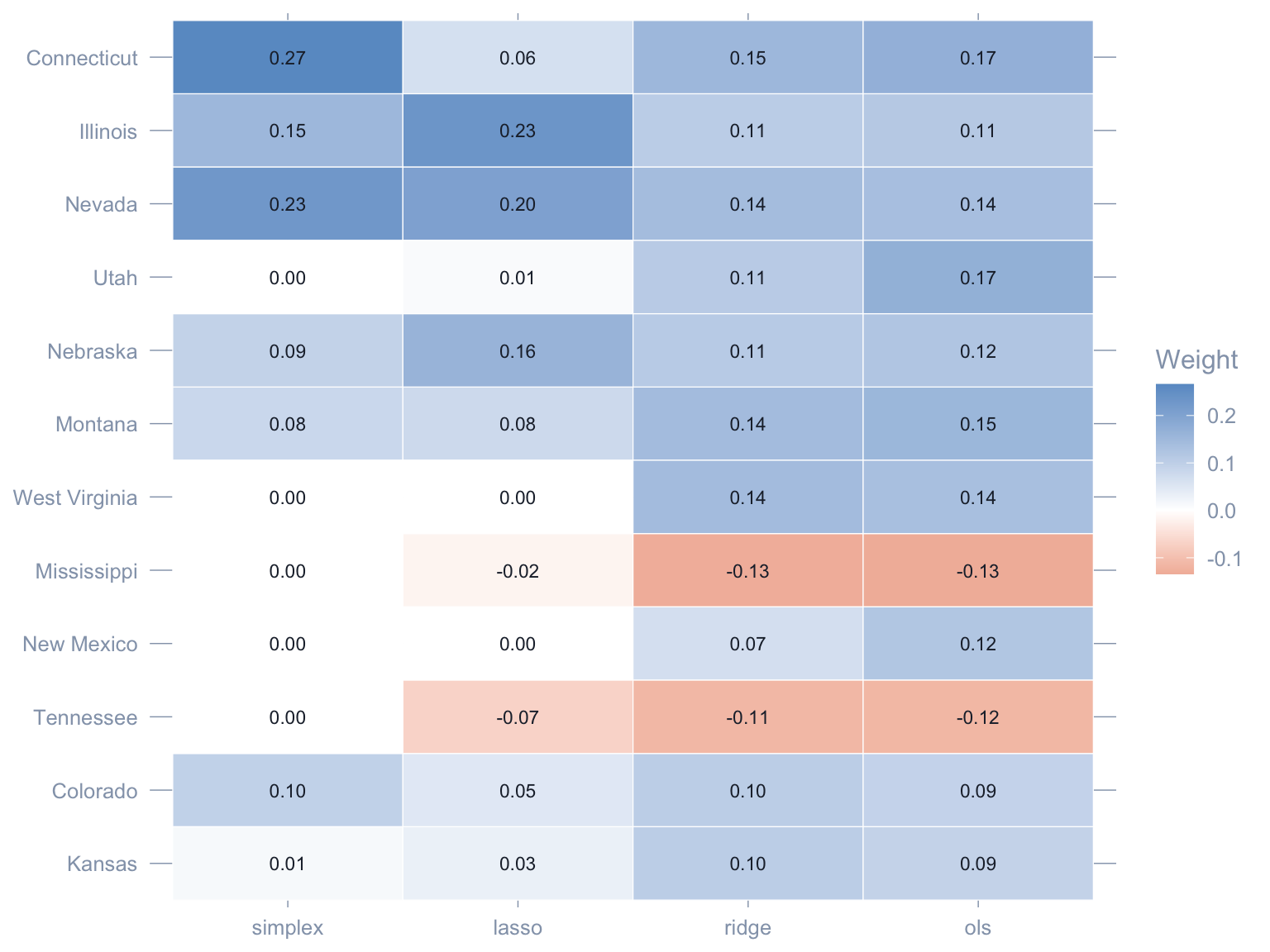
Three readings emerge.
1. **Simplex is the sparsest.** Four to five donors absorb essentially the entire weight; the rest are pinned to zero by the non-negativity and sum-to-one constraints. This is the chapter 4 picture.
2. **OLS and lasso admit negative weights.** Once we drop the simplex, some donors enter with sign-flipped contributions that pull the synthetic in the opposite direction. Whether that is *interpretable* (a "shorted" donor) or *artefactual* (overfitting to noise on a 19-year pre-period) is a real modelling decision.
3. **Ridge is the smoothest.** The L2 penalty spreads weight more evenly across the donor pool, producing a synthetic that depends on dozens of states rather than a handful.
```{r}
#| label: fig-weights-heatmap
#| fig-cap: "Donor weights across the four scpi constraints, displayed as a heatmap, for the 12 donors with largest maximum absolute weight across constraints. Rows are donors; columns are constraints. Red = negative weight, blue = positive."
#| fig-width: 8
#| fig-height: 6
#| code-summary: "Code: Plot a heatmap of donor weights across constraints for the top-12 donors."
top_states <- weight_wide |>
  mutate(rank_score = pmax(abs(simplex), abs(lasso), abs(ridge), abs(ols))) |>
  arrange(desc(rank_score)) |>
  head(12) |>
  pull(state)

weight_long |>
  filter(state %in% top_states) |>
  mutate(
    state      = factor(state, levels = rev(top_states)),
    constraint = factor(constraint, levels = constraints)
  ) |>
  ggplot(aes(x = constraint, y = state, fill = weight)) +
  geom_tile(color = "white") +
  geom_text(aes(label = sprintf("%.2f", weight)), size = 3,
            color = "#1f2937") +
  scale_fill_gradient2(low = "#d97757", mid = "white",
                       high = "#6a9bcc", midpoint = 0) +
  labs(x = NULL, y = NULL, fill = "Weight") +
  theme(legend.position = "right",
        panel.grid       = element_blank())
```
## Synthetic counterfactuals across constraints
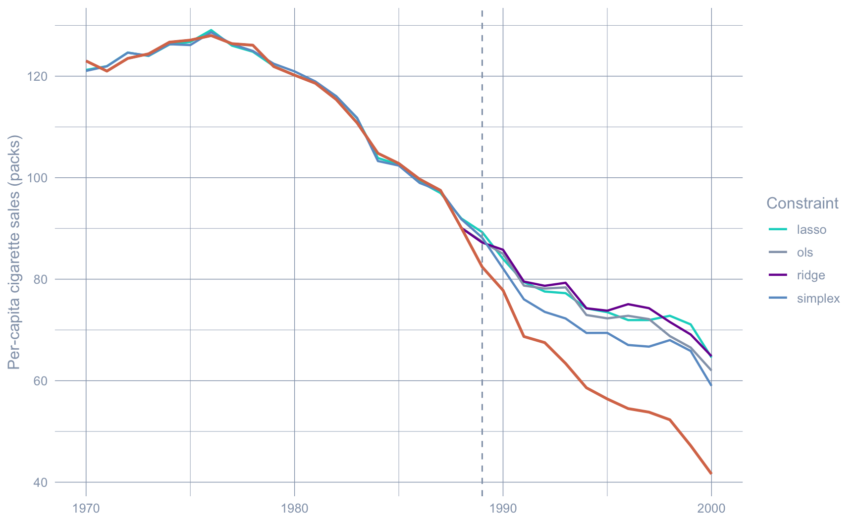
The point of the weight comparison is not aesthetics — it is to ask whether the *fitted synthetic counterfactual* depends on the choice of constraint. The next plot overlays the four synthetic series on the observed California trajectory.
```{r}
#| label: fig-counterfactuals
#| fig-cap: "Observed California (orange) and the four scpi synthetic counterfactuals (one per constraint). Pre-1989 the four synthetics are nearly indistinguishable; post-1989 they fan out but all sit visibly above observed California."
#| fig-width: 9
#| fig-height: 5.5
#| code-summary: "Code: Overlay observed California against the four synthetic counterfactual series."
years_pre  <- 1970:1988
years_post <- 1989:2000
years_all  <- c(years_pre, years_post)

extract_synth <- function(fit, name) {
  pre  <- as.numeric(fit$est.results$Y.pre.fit)
  post <- as.numeric(fit$est.results$Y.post.fit)
  tibble(
    year       = years_all,
    synthetic  = c(pre, post),
    constraint = name
  )
}

synth_long <- imap_dfr(scest_fits, \(fit, name) extract_synth(fit, name))

observed <- tibble(
  year     = years_all,
  observed = c(
    as.numeric(data_prep$Y.pre),
    as.numeric(data_prep$Y.post)
  )
)

ggplot() +
  geom_line(data = synth_long,
            aes(x = year, y = synthetic, color = constraint),
            linewidth = 0.8) +
  geom_line(data = observed,
            aes(x = year, y = observed),
            color = "#d97757", linewidth = 1) +
  geom_vline(xintercept = 1989, linetype = "dashed", color = "#94a3b8") +
  scale_color_manual(values = c(
    simplex = "#6a9bcc", lasso = "#00d4c8",
    ridge   = "#7A209F", ols   = "#94a3b8"
  )) +
  labs(x = NULL, y = "Per-capita cigarette sales (packs)",
       color = "Constraint")
```
The pre-period overlap is near-perfect — every constraint can fit 19 years of California data to within a few packs. The post-period spread is the interesting part: simplex and lasso land in roughly the same place, ridge sits slightly higher, OLS sits slightly lower. The point estimate of the ATT is mildly sensitive to the constraint; the *sign and order of magnitude* are not.
```{r}
#| label: tbl-att-by-constraint
#| tbl-cap: "Average post-period gap (ATT) by weight constraint."
#| code-summary: "Code: Summarise the average, minimum, and maximum post-period gap per constraint."
att_by_constraint <- imap_dfr(scest_fits, \(fit, name) {
  gap <- as.numeric(data_prep$Y.post) - as.numeric(fit$est.results$Y.post.fit)
  tibble(constraint = name, ATT = mean(gap),
         min_gap = min(gap), max_gap = max(gap))
})

att_by_constraint |>
  gt_pretty(decimals = 2) |>
  gt::cols_label(constraint = "Constraint", ATT = "Average post-period gap",
                 min_gap = "Min gap", max_gap = "Max gap")
```
```{r}
#| label: att-pull
#| echo: false
att_lookup <- setNames(att_by_constraint$ATT, att_by_constraint$constraint)
att_simplex <- att_lookup[["simplex"]]
att_lasso <- att_lookup[["lasso"]]
att_ridge <- att_lookup[["ridge"]]
att_ols <- att_lookup[["ols"]]
deepest_gap <- min(att_by_constraint$min_gap)
ypost_mean <- mean(as.numeric(data_prep$Y.post))
pct_simplex <- 100 * abs(att_simplex) / ypost_mean
pct_ridge <- 100 * abs(att_ridge) / ypost_mean
```
All four estimators place the average post-period gap between roughly `r sprintf("%.1f", min(att_lookup))` and `r sprintf("%.1f", max(att_lookup))` packs/capita per year, with year-by-year gaps as deep as `r sprintf("%.1f", deepest_gap)` in the late 1990s. The simplex sits at the conservative end of that range ($\widehat{\tau}_{\text{scpi-simplex}} \approx `r sprintf("%.2f", att_simplex)`$), lasso and ridge sit at the negative end ($\widehat{\tau}_{\text{scpi-lasso}} \approx `r sprintf("%.2f", att_lasso)`$ and $\widehat{\tau}_{\text{scpi-ridge}} \approx `r sprintf("%.2f", att_ridge)`$), and OLS lands in between ($\widehat{\tau}_{\text{scpi-ols}} \approx `r sprintf("%.2f", att_ols)`$). On a post-period baseline of $\approx `r sprintf("%.0f", ypost_mean)`$ packs/capita per year, those gaps correspond to a `r sprintf("%.0f", pct_simplex)`–`r sprintf("%.0f", pct_ridge)`% reduction. Whatever one believes about the simplex, Proposition 99 reduced California cigarette sales by an economically meaningful share of pre-policy consumption.
A reader paging back from chapter 4 will notice that $\widehat{\tau}_{\text{scpi-simplex}}$ here (≈ `r sprintf("%.2f", att_simplex)`) is materially smaller in magnitude than chapter 4's simplex ATT ($\widehat{\tau}_{\text{SCM}} \approx -18.85$). Three things drive that gap: (i) chapter 4 used `lnincome`, `beer`, and `age15to24` as auxiliary predictors via `tidysynth::generate_predictor()`, while this chapter matches on the outcome series alone (see *Setup and data* above); (ii) the two chapters use different solvers (`tidysynth`/`Synth` quadratic optimiser vs `scpi`'s constrained-least-squares routine); and (iii) `scpi` fits with `constant = TRUE`, adding a single intercept across features. Predictor-augmented matching extracts more pre-period signal and therefore produces a more negative ATT; outcome-only matching is the more conservative — and more honest — choice when the auxiliary covariates are themselves heavily missing on the donor side. The two numbers do not contradict each other; they answer slightly different questions about the same data.
## Prediction intervals on the simplex fit
`scpi()` is the inference-bearing sibling of `scest()`. It rebuilds the same synthetic counterfactual and adds a prediction interval. The argument settings below — `u.order = 1`, `u.lags = 0`, `e.order = 1`, `e.lags = 0`, `u.missp = TRUE`, `u.sigma = "HC1"`, `sims = 200` — are the package defaults. We override `e.method = "gaussian"` (the package default is `"all"`, which computes Gaussian, location-scale, and quantile-regression bounds simultaneously) because the Gaussian conditional subgaussian bound is the version proved in @cattaneo2021prediction and is the simplest to interpret for a single-treated-unit panel.
**A note on confidence levels.** Setting `u.alpha = 0.025` and `e.alpha = 0.025` yields a $\widehat{\text{PI}}_{1t}$ that is *jointly* conservative at level $1 - (u_\alpha + e_\alpha) = 95\%$ by a Bonferroni-style union bound: the in-sample weight error $(w^* - \widehat{w})^\top Y_{0t}$ and the out-of-sample shock $e_t$ are each bounded at the $1 - 0.025 = 97.5\%$ level, so the joint coverage is at least $1 - 2 \times 0.025 = 95\%$. Equivalently, to obtain a joint $(1 - \alpha)$ band we split alpha as `u.alpha = e.alpha = α/2`. We follow this convention throughout the chapter so that "95% PI" really does mean "95% joint coverage"; the sensitivity analysis later in the chapter sweeps the joint level directly.
```{r}
#| label: scpi-simplex
#| message: false
#| warning: false
#| results: hide
#| code-summary: "Code: Fit scpi with the simplex constraint and a 95% joint Gaussian prediction interval."
set.seed(42)
pi_simplex <- scpi(
  data_prep,
  w.constr   = list(name = "simplex"),
  u.order    = 1, u.lags = 0,
  e.order    = 1, e.lags = 0,
  e.method   = "gaussian",
  u.missp    = TRUE,
  u.sigma    = "HC1",
  e.alpha    = 0.025,
  u.alpha    = 0.025,
  sims       = 200
)
```
The simplex `scpi` object carries the same point-estimate slots as `scest_fits$simplex` plus an `inference.results` block with the Gaussian-method 95% joint $\widehat{\text{PI}}_{1t}$ lower (`CI.all.gaussian[, 1]`) and upper (`CI.all.gaussian[, 2]`) bounds for each post-period year.
```{r}
#| label: fig-pi-simplex
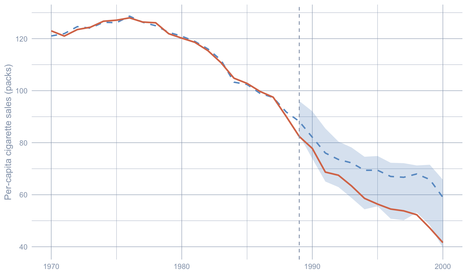
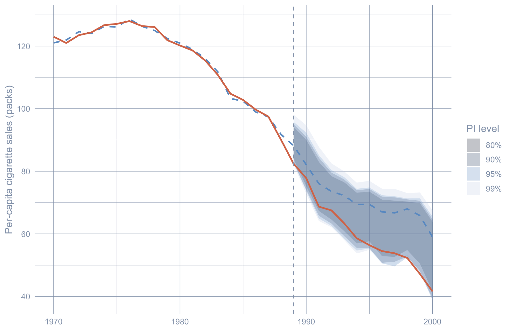
#| fig-cap: "Simplex synthetic-control fit (blue dashed) for California (orange solid) with the 95% joint scpi prediction interval (blue PI band). Observed California falls below the lower PI bound from roughly the mid-1990s onward — the inferential analogue of \"effect statistically distinguishable from forecasting noise\"."
#| fig-width: 8.5
#| fig-height: 5
#| warning: false
#| code-summary: "Code: Plot the simplex synthetic, observed California, and the 95% joint PI band."
ci_post <- pi_simplex$inference.results$CI.all.gaussian
synth_pre  <- as.numeric(pi_simplex$est.results$Y.pre.fit)
synth_post <- as.numeric(pi_simplex$est.results$Y.post.fit)

pi_df <- tibble(
  year      = years_all,
  observed  = c(as.numeric(data_prep$Y.pre), as.numeric(data_prep$Y.post)),
  synthetic = c(synth_pre, synth_post),
  ci_lo     = c(rep(NA_real_, length(years_pre)), ci_post[, 1]),
  ci_hi     = c(rep(NA_real_, length(years_pre)), ci_post[, 2])
)

ggplot(pi_df, aes(x = year)) +
  geom_ribbon(aes(ymin = ci_lo, ymax = ci_hi),
              fill = "#6a9bcc", alpha = 0.25) +
  geom_line(aes(y = synthetic), color = "#6a9bcc",
            linewidth = 0.9, linetype = "dashed") +
  geom_line(aes(y = observed), color = "#d97757", linewidth = 1) +
  geom_vline(xintercept = 1989, linetype = "dashed", color = "#94a3b8") +
  labs(x = NULL, y = "Per-capita cigarette sales (packs)")
```
The pre-period synthetic tracks observed California almost perfectly. After 1989 the PI band fans out as the out-of-sample forecast horizon lengthens — that is $e_t$ at work. Observed California breaks below the lower bound by the early-to-mid 1990s and stays there. Under the SCPI framework that is the formal version of the statement chapter 4 made loosely with the placebo cloud: the post-1989 trajectory is not what synthetic California, plus its honest forecast error, would produce.
## Prediction intervals across all four constraints
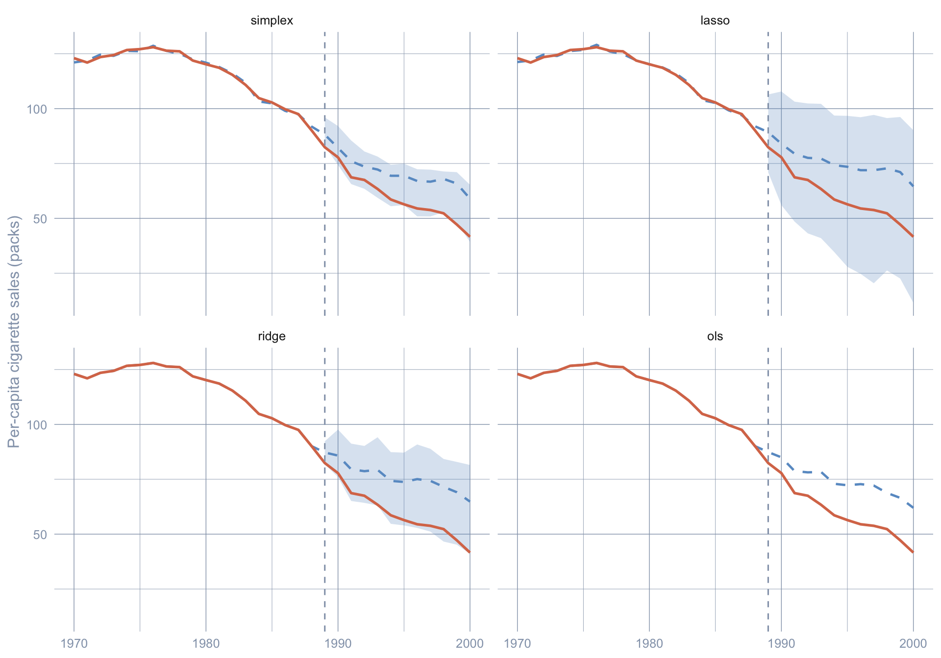
The substantive question — is the effect robust across constraints — also has a sharper inferential form. We can ask whether observed California falls below the *lower PI bound* under simplex, lasso, ridge, and OLS alike.
```{r}
#| label: scpi-all
#| message: false
#| warning: false
#| results: hide
#| code-summary: "Code: Fit scpi with prediction intervals under all four weight constraints."
set.seed(42)
scpi_fits <- map(constraints, \(name) {
  scpi(
    data_prep,
    w.constr = list(name = name),
    u.order  = 1, u.lags = 0,
    e.order  = 1, e.lags = 0,
    e.method = "gaussian",
    u.missp  = TRUE,
    u.sigma  = "HC1",
    e.alpha  = 0.025, u.alpha = 0.025,
    sims     = 200
  )
}) |>
  set_names(constraints)
```
```{r}
#| label: fig-pi-all
#| fig-cap: "Observed California (orange) versus the 95% joint prediction interval (blue PI band) and synthetic point estimate (blue dashed) under each scpi weight constraint. The lower-bound piercing in the late 1990s survives every constraint family."
#| fig-width: 10
#| fig-height: 7
#| warning: false
#| code-summary: "Code: Facet the synthetic fit and 95% PI band across all four constraints."
pi_all <- imap_dfr(scpi_fits, \(fit, name) {
  ci <- fit$inference.results$CI.all.gaussian
  tibble(
    year      = years_all,
    constraint = name,
    observed  = c(as.numeric(data_prep$Y.pre), as.numeric(data_prep$Y.post)),
    synthetic = c(as.numeric(fit$est.results$Y.pre.fit),
                  as.numeric(fit$est.results$Y.post.fit)),
    ci_lo     = c(rep(NA_real_, length(years_pre)), ci[, 1]),
    ci_hi     = c(rep(NA_real_, length(years_pre)), ci[, 2])
  )
}) |>
  mutate(constraint = factor(constraint, levels = constraints))

ggplot(pi_all, aes(x = year)) +
  geom_ribbon(aes(ymin = ci_lo, ymax = ci_hi),
              fill = "#6a9bcc", alpha = 0.25) +
  geom_line(aes(y = synthetic), color = "#6a9bcc",
            linewidth = 0.85, linetype = "dashed") +
  geom_line(aes(y = observed), color = "#d97757", linewidth = 0.95) +
  geom_vline(xintercept = 1989, linetype = "dashed", color = "#94a3b8") +
  facet_wrap(~ constraint, nrow = 2) +
  labs(x = NULL, y = "Per-capita cigarette sales (packs)")
```
The PI-band widths differ — OLS is the widest because unconstrained least squares squeezes the most variance out of the pre-period and pays for it with a fatter post-period interval, while simplex is the narrowest because the non-negativity-plus-sum-to-one constraint sharply regularises the donor weights. Yet observed California eventually slips below every constraint's lower band. The inferential conclusion does not depend on the modelling choice that chapter 4 hard-coded.
## Sensitivity to confidence level
The 95% band is a convention. A second robustness check is to sweep the joint confidence level $1 - (u_\alpha + e_\alpha)$ across reasonable values and ask when the observed series finally re-enters the band. Wider bands (higher confidence) make the post-period evidence weaker; narrower bands (lower confidence) make it stronger. To keep the labels honest, we set `u.alpha = e.alpha = α/2` so that the joint Bonferroni level is exactly $1 - \alpha$ — i.e. a labelled "90% PI" really does have 90% joint coverage.
```{r}
#| label: scpi-sensitivity
#| message: false
#| warning: false
#| results: hide
#| code-summary: "Code: Refit simplex scpi across joint confidence levels of 80, 90, 95, and 99 percent."
set.seed(42)
alpha_levels <- c(0.20, 0.10, 0.05, 0.01)

sens_fits <- map(alpha_levels, \(a) {
  scpi(
    data_prep,
    w.constr = list(name = "simplex"),
    u.order  = 1, u.lags = 0,
    e.order  = 1, e.lags = 0,
    e.method = "gaussian",
    u.missp  = TRUE,
    u.sigma  = "HC1",
    e.alpha  = a / 2, u.alpha = a / 2,
    sims     = 200
  )
}) |>
  set_names(paste0(100 * (1 - alpha_levels), "%"))
```
```{r}
#| label: fig-sensitivity
#| fig-cap: "Sensitivity to the joint confidence level (simplex constraint). Nested bands at 80%, 90%, 95%, and 99%. Observed California (orange) sits below the lower bound at every level by the late 1990s."
#| fig-width: 8.5
#| fig-height: 5.5
#| code-summary: "Code: Plot the nested PI bands at 80, 90, 95, and 99 percent confidence levels."
sens_df <- imap_dfr(sens_fits, \(fit, lvl) {
  ci <- fit$inference.results$CI.all.gaussian
  tibble(
    year  = years_post,
    level = lvl,
    ci_lo = ci[, 1],
    ci_hi = ci[, 2]
  )
}) |>
  mutate(level = factor(level, levels = paste0(100 * (1 - alpha_levels), "%")))

obs_df <- tibble(year = years_all,
                 observed = c(as.numeric(data_prep$Y.pre),
                              as.numeric(data_prep$Y.post)))
synth_df <- tibble(year = years_all,
                   synthetic = c(synth_pre, synth_post))

ggplot() +
  geom_ribbon(data = sens_df,
              aes(x = year, ymin = ci_lo, ymax = ci_hi, fill = level),
              alpha = 0.25) +
  geom_line(data = synth_df, aes(x = year, y = synthetic),
            color = "#6a9bcc", linetype = "dashed", linewidth = 0.85) +
  geom_line(data = obs_df, aes(x = year, y = observed),
            color = "#d97757", linewidth = 0.95) +
  geom_vline(xintercept = 1989, linetype = "dashed", color = "#94a3b8") +
  scale_fill_manual(values = c(
    "80%" = "#0b1d33", "90%" = "#1f4068",
    "95%" = "#6a9bcc", "99%" = "#cdd9eb"
  )) +
  labs(x = NULL, y = "Per-capita cigarette sales (packs)", fill = "PI level")
```
The narrow 80% band is broken by the early 1990s; the widest 99% band still excludes observed California by the late 1990s. The post-1989 deviation is not a 95%-only artefact.
## Common pitfalls
**Reading $\widehat{\text{PI}}_{1t}$ as a confidence interval for the treatment effect.** An `scpi` prediction interval covers the *synthetic counterfactual* $\widehat{Y_{1t}(0)}$ — it tells you the range of values the synthetic-California series could plausibly take if you re-ran the donor-weight estimator on a parallel pre-period draw. The treatment effect $\widehat{\tau}_t = Y_{1t} - \widehat{Y_{1t}(0)}$ "matters" when observed California leaves the band: that is the inferential statement. Reading the band as a $\pm$ on the *effect size* (the way one would read an OLS confidence interval on a regression coefficient) is wrong, and it is the most common misuse of the package in applied work. Exercise 3 shows the formal way to flip the band onto $\widehat{\tau}_t$: subtract the band endpoints from $Y_{1t}$ (with bounds swapped) rather than re-centring the band on $\widehat{\tau}_t$.
**Treating the constraint choice as innocuous.** Simplex, lasso, ridge, and OLS are not interchangeable. In the run above $\widehat{\tau}_{\text{scpi-simplex}}$ and $\widehat{\tau}_{\text{scpi-ridge}}$ differ by roughly 5 packs (a 40% relative spread on the point estimate). The *inferential* conclusion happens to survive every constraint family here, but on a borderline-significant dataset it would not. Pick the constraint before you peek at the post-period and report the others as robustness checks; do not constraint-shop until a desired sign emerges. Relatedly, the lasso fits here use scpi's default $Q = 1$, which is what gives lasso and simplex such similar weight vectors (lasso = "L1 ball of radius 1"; simplex = "L1 ball of radius 1, restricted to the non-negative orthant"). Pushing $Q$ above 1 lets lasso assign weight outside the simplex on either side and changes the picture. A serious lasso analysis would sweep $Q$ over a grid (exercise 5); we keep $Q = 1$ here for comparability with the simplex.
**PIs are conditional on the donor pool.** `scpi` quantifies in-sample and out-of-sample error *given* the 38 donor states that survived the data-quality screen. The interval makes no statement about whether the donor pool itself is reasonable — adding or removing a state, or shifting the pre-period window, can move both $\widehat{\tau}_{\text{scpi}}$ and the band. The honest reading is that $\widehat{\text{PI}}_{1t}$ is "frequentist coverage for the counterfactual implied by *this* donor pool"; sensitivity to pool composition is a separate exercise (placebos, leave-one-out, donor-restriction sweeps).
**PI bands grow rapidly with horizon in a small-T regime.** With only 19 pre-period years and 12 post-period years, the out-of-sample component $e_t$ grows quickly: by 2000 the simplex band is several times wider than the 1990 band. A reader who looks only at the late-1990s years sees a large interval and may infer "weak evidence"; the inferential signal is concentrated in the *first few* post-period years, where the band is narrow and the gap is already opening. Always read the PI plot as a function of horizon, not as a single late-period interval.
## Recap
| Question | Answer |
|---|---|
| What does this chapter add over chapter 4? | Frequentist prediction intervals $\widehat{\text{PI}}_{1t}$ with finite-sample coverage, plus three alternatives to the simplex (lasso, ridge, OLS) |
| What is the simplex point ATT? | $\widehat{\tau}_{\text{scpi-simplex}} \approx `r sprintf("%.2f", att_simplex)`$ packs/capita per year, 1989–2000 (outcome-only matching; cf. chapter 4's $\widehat{\tau}_{\text{SCM}} \approx -18.85$ with predictor-augmented matching) |
| Does the ATT survive the constraint choice? | Yes — all four constraints produce a negative average gap between roughly `r sprintf("%.1f", min(att_lookup))` and `r sprintf("%.1f", max(att_lookup))` packs |
| Does the *inferential* conclusion survive? | Yes — observed California falls below the lower 95% joint PI bound under every constraint by the late 1990s |
| What does $\widehat{\text{PI}}_{1t}$ cover? | The *synthetic counterfactual* $\widehat{Y_{1t}(0)}$, not observed California and not $\widehat{\tau}_t$ — "significance" means the observed series leaves the band |
| How does this differ from chapter 7's credible interval? | $\widehat{\text{PI}}_{1t}$ has finite-sample frequentist coverage and is a statement about the synthetic counterfactual; CausalImpact's CrI is a posterior probability statement about the effect, conditioned on the prior. They tend to agree when the BSTS prior is uninformative and the SCPI in-sample uncertainty term dominates. |
| What is the most important `scpi` switch for this dataset? | `cointegrated.data = TRUE`, which adjusts the long-run variance for the I(1)-looking `cigsale` series |
| What is the design-time pitfall? | Adding covariates with NAs (`beer`, `age15to24`, `lnincome`) forces row deletions that bias the donor pool; the chapter uses outcome-only matching |
## Key takeaways
**Methods:**
- `scpi` fits the synthetic-control predictor $\widehat{Y_{1t}(0)} = \widehat{w}^\top Y_{0t}$ under a chosen donor-weight constraint (simplex, lasso, ridge, or OLS) and constructs a finite-sample prediction interval $\widehat{\text{PI}}_{1t}$ by decomposing the forecast error into two components: an in-sample piece $(w^* - \widehat{w})^\top Y_{0t}$ that captures donor-weight estimation variability over a finite pre-period, and an out-of-sample piece $e_t$ that captures post-treatment shocks unknowable from the pre-period.
- Splitting the joint level as `u.alpha = e.alpha = α/2` delivers a Bonferroni-style $(1-\alpha)$ band over both error sources; the simplex weights here additionally satisfy the Abadie–Diamond–Hainmueller constraints $\widehat{w}_j \geq 0$ and $\sum_j \widehat{w}_j = 1$, so the synthetic remains a convex combination of donor states.
- $\widehat{\text{PI}}_{1t}$ covers the synthetic counterfactual $\widehat{Y_{1t}(0)}$ — not $\widehat{\tau}_t$ and not a rank-based null distribution; "significance" is signalled when observed California leaves the band, in contrast to chapter 4's Fisher placebo test, which ranks the treated unit against permuted-treatment donors without modelling either error source and so returns a $p$-value rather than an interval.
**Lessons:**
- Across simplex, lasso, ridge, and OLS, $\widehat{\tau}_{\text{scpi-simplex}}$ lands at ≈ `r sprintf("%.2f", att_simplex)` packs/capita while the other three constraints reach ≈ `r sprintf("%.2f", min(att_lookup))` — a 40% relative spread on the point estimate, yet observed California falls below the lower 95% joint PI bound under every constraint family by the late 1990s, so the inferential conclusion is robust even when the point estimate is not.
- $\widehat{\tau}_{\text{scpi-simplex}}$ here (≈ `r sprintf("%.2f", att_simplex)`) is materially less negative than chapter 4's $\widehat{\tau}_{\text{SCM}} \approx -18.85$ because this chapter matches on the outcome alone, omits the auxiliary predictors `lnincome`, `beer`, and `age15to24` that carried NAs in the early pre-period, and uses scpi's constrained-least-squares solver with `constant = TRUE`; outcome-only matching is the more honest — and more conservative — choice when covariates would force row deletions on the donor side.
- PI bands can be *narrower* than the placebo cloud chapter 4 would suggest when the in-sample component is small (tight pre-period fit, well-regularised donor pool, as with the simplex) and *wider* when it is large (OLS pays for an unconstrained pre-period fit with a fatter post-period band); sweeping the joint confidence level from 80% to 99% leaves the lower-bound piercing intact by the late 1990s, so the post-1989 deviation is not a 95%-only artefact.
**Caveats:**
- Finite-sample coverage depends on the assumed distribution of the post-treatment shock $e_t$ — the chapter uses `e.method = "gaussian"` (the conditional-subgaussian bound proved in @cattaneo2021prediction), and a fatter-tailed shock distribution would deliver weaker coverage than the nominal level claims; conformal-inference alternatives (Chernozhukov, Wüthrich & Zhu 2021) trade the parametric decomposition for distribution-free quantile guarantees.
- $\widehat{\text{PI}}_{1t}$ is conditional on the donor pool and grows rapidly with horizon in a small-T regime — with only 19 pre-period years the out-of-sample component dominates by 2000, and the band makes no statement about whether the 38-state donor pool is itself reasonable; pool composition, pre-period window, and the lasso tuning parameter $Q$ (held at the package default $Q = 1$ here) are sensitivities the PI does not absorb.
- Reading the band as a $\pm$ on the *effect size* — the way one would read an OLS confidence interval on a regression coefficient — is the most common applied misuse of `scpi`; the band is a region for the counterfactual, so the implied uncertainty on $\widehat{\tau}_t = Y_{1t} - \widehat{Y_{1t}(0)}$ is the mirror-image gap between the observed series and the band (exercise 3), not the band's half-width.
## Further reading
- @cattaneo2021prediction — the JASA paper that introduced the SCPI framework and proves the finite-sample coverage guarantee.
- @cattaneo2025scpi — the JSS software paper for the R and Python implementations; the chapter's argument defaults are taken from its replication script.
- @abadie2021using — JEL methodological review covering feasibility, data requirements, and assumptions for classical SCM (the baseline this chapter relaxes).
- @dunford2024tidysynth — the `tidysynth` package used in chapter 4, for direct A/B comparison with the simplex pipeline run here.
- Chernozhukov, V., Wüthrich, K. & Zhu, Y. (2021). *An exact and robust conformal inference method for counterfactual and synthetic controls.* Journal of the American Statistical Association — a distribution-free frequentist alternative to scpi's parametric in-sample / out-of-sample decomposition. Conformal SC intervals trade scpi's two-component parametric coverage for permutation-style quantile guarantees and are a natural companion read.
- The companion **Python (`scpi_pkg`) and Stata (`scpi`)** packages, documented at <https://nppackages.github.io/scpi/>, expose the same API as the R package used in this chapter.
**Coming up.** Chapter 7 closes Part I with a *fourth* synthetic-control perspective: a Bayesian horseshoe-prior weight model coupled with a spatial-autoregressive donor data-generating process. Chapters 4, 5, and 6 all retain the stable-unit-treatment-value assumption (SUTVA) — donors are treated as unaffected by California's policy. Chapter 7 relaxes SUTVA and recovers a closed-form spillover for each neighbour, which matters when the treated unit shares a border with several donors (Nevada, in this case).
## Exercises
These exercises probe the design knobs the chapter exposed — the cointegration flag, the constraint family, the Bonferroni alpha allocation, and the lasso $Q$ tuning parameter — and one summary statistic the chapter did not extract (the first year California pierces the lower band). All exercises reuse `prop99`, `data_prep`, `pi_simplex`, `scpi_fits`, `years_pre`, `years_post`, and `years_all` from the setup chunks above.
### Exercise 1: Cointegration toggle
The chapter ran `scdata(..., cointegrated.data = TRUE)` because California's per-capita cigarette sales look like an I(1) series. Refit the simplex `scpi` with `cointegrated.data = FALSE` and compare the average PI half-width across the post-period. How much does the cointegration adjustment matter?
::: {.callout-tip collapse="true"}
## Solution
```{r}
#| label: ex-ch08-01
#| message: false
#| warning: false
#| results: hide
data_prep_nocoint <- scdata(
  df               = prop99,
  id.var           = "state",
  time.var         = "year",
  outcome.var      = "cigsale",
  period.pre       = 1970:1988,
  period.post      = 1989:2000,
  unit.tr          = "California",
  unit.co          = donors,
  cointegrated.data = FALSE,
  constant         = TRUE
)

set.seed(42)
pi_nocoint <- scpi(
  data_prep_nocoint,
  w.constr = list(name = "simplex"),
  u.order  = 1, u.lags = 0,
  e.order  = 1, e.lags = 0,
  e.method = "gaussian",
  u.missp  = TRUE, u.sigma = "HC1",
  e.alpha  = 0.025, u.alpha = 0.025,
  sims     = 200
)
```
```{r}
#| label: ex-ch08-01b
ci_yes <- pi_simplex$inference.results$CI.all.gaussian
ci_no  <- pi_nocoint$inference.results$CI.all.gaussian

tibble(setting       = c("cointegrated = TRUE (chapter)",
                         "cointegrated = FALSE"),
       mean_halfwidth = c(mean((ci_yes[, 2] - ci_yes[, 1]) / 2),
                          mean((ci_no[, 2]  - ci_no[, 1])  / 2))) |>
  gt_pretty(decimals = 2)
```
Turning off the cointegration adjustment shrinks the average PI half-width somewhat: the long-run-variance correction inflates the in-sample uncertainty component to account for the high serial correlation of an I(1) outcome. The chapter's `TRUE` is the more honest default for `cigsale`; setting it to `FALSE` gives a narrower band that can mislead readers into thinking the post-1989 effect is more sharply identified than it actually is.
:::
### Exercise 2: First post-period year California pierces the lower PI bound
For each of the four constraints, find the first post-period year in which observed California falls *below* the lower 95% PI bound. This is the inferential analogue of "the year the effect became statistically distinguishable from forecasting noise."
::: {.callout-tip collapse="true"}
## Solution
```{r}
#| label: ex-ch08-02
y_post <- as.numeric(data_prep$Y.post)

first_exit <- function(fit) {
  ci <- fit$inference.results$CI.all.gaussian
  below <- y_post < ci[, 1]
  below[is.na(below)] <- FALSE
  if (!any(below)) NA_integer_ else as.integer(years_post[which(below)[1]])
}

tibble(constraint = constraints,
       first_year = map_int(scpi_fits, first_exit)) |>
  gt_pretty()
```
Every constraint shows observed California falling below the lower PI bound by the early-to-mid 1990s. The simplex and lasso fits give the earliest first-exit year (their bands are narrowest); ridge and OLS push the first-exit year out by a year or two (their bands are wider). The constraint choice affects *when* the inferential break opens but not *whether* it opens — a robustness signal stronger than the point-estimate spread alone.
:::
### Exercise 3: Per-year treatment-effect interval
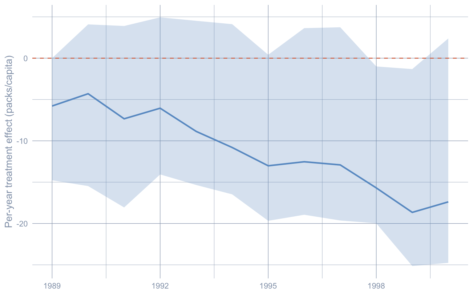
The chapter plotted $\widehat{\text{PI}}_{1t}$ around the *synthetic counterfactual* $\widehat{Y_{1t}(0)}$. Reframe it: plot the implied band around the per-year *treatment effect* $\widehat{\tau}_t = Y_{1t} - \widehat{Y_{1t}(0)}$. Since $Y_{1t}$ is observed, the upper bound on $\widehat{\tau}_t$ is $Y_{1t}$ minus the *lower* PI bound on the counterfactual, and vice versa. The horizontal zero line then anchors the eye: years whose band stays below zero are the years the policy effect is statistically distinguishable from zero.
::: {.callout-tip collapse="true"}
## Solution
```{r}
#| label: ex-ch08-03
#| fig-width: 8
#| fig-height: 5
ci_post <- pi_simplex$inference.results$CI.all.gaussian
synth_post <- as.numeric(pi_simplex$est.results$Y.post.fit)

tau_df <- tibble(
  year     = years_post,
  observed = y_post,
  tau      = observed - synth_post,
  tau_lo   = observed - ci_post[, 2],
  tau_hi   = observed - ci_post[, 1]
)

ggplot(tau_df, aes(year, tau)) +
  geom_ribbon(aes(ymin = tau_lo, ymax = tau_hi),
              fill = "#6a9bcc", alpha = 0.25) +
  geom_line(color = "#6a9bcc", linewidth = 0.9) +
  geom_hline(yintercept = 0, color = "#d97757", linetype = "dashed") +
  labs(x = NULL, y = "Per-year treatment effect (packs/capita)")
```
The point-effect series drops steadily through the post-period; the upper bound of the band first dips below zero in the mid-1990s and stays there. The visual is strictly equivalent to the chapter's "California below the lower bound" framing — but with zero on the y-axis, the inferential break shows up as a band that has cleared zero, which many readers find more direct.
:::
### Exercise 4: Asymmetric Bonferroni alpha allocation
The chapter splits a 95% joint band evenly (`u.alpha = e.alpha = 0.025`). Refit the simplex `scpi` with an *asymmetric* split: `u.alpha = 0.04` and `e.alpha = 0.01` (still summing to 0.05). The total Bonferroni level is still 95%, but the shape of the band changes — one source of uncertainty is now bounded more tightly than the other. Compare to the symmetric chapter band.
::: {.callout-tip collapse="true"}
## Solution
```{r}
#| label: ex-ch08-04
#| message: false
#| warning: false
#| results: hide
set.seed(42)
pi_asym <- scpi(
  data_prep,
  w.constr = list(name = "simplex"),
  u.order  = 1, u.lags = 0,
  e.order  = 1, e.lags = 0,
  e.method = "gaussian",
  u.missp  = TRUE, u.sigma = "HC1",
  u.alpha  = 0.04,
  e.alpha  = 0.01,
  sims     = 200
)
```
```{r}
#| label: ex-ch08-04b
ci_sym  <- pi_simplex$inference.results$CI.all.gaussian
ci_asym <- pi_asym$inference.results$CI.all.gaussian

tibble(
  year             = years_post,
  width_symmetric  = ci_sym[, 2]  - ci_sym[, 1],
  width_asymmetric = ci_asym[, 2] - ci_asym[, 1]
) |>
  gt_pretty(decimals = 2)
```
The asymmetric band trades a tighter out-of-sample bound (`e.alpha = 0.01`) for a looser in-sample bound (`u.alpha = 0.04`). On a 19-year pre-period with 12 post-period years, the in-sample component dominates by mid-horizon, so loosening it *widens* the band where it already mattered most. This is the lesson of the Bonferroni union bound: the split is yours to choose, but you cannot get both bounds tight for free. Symmetric is the conservative default; asymmetric splits make sense only when you have a substantive reason to trust one of the two error sources more than the other.
:::
### Exercise 5 (stretch): Lasso $Q$ sweep
The chapter's lasso fit uses `scpi`'s default $Q = 1$, which is what makes the lasso weights look so similar to the simplex weights ("lasso = L1 ball of radius 1; simplex = L1 ball of radius 1 restricted to the non-negative orthant"). Sweep $Q$ over $\{0.5, 1, 2\}$, refit `scpi` at each value, and report the resulting ATT plus the number of donors with non-zero weight (the lasso's "active set" size).
::: {.callout-tip collapse="true"}
## Solution
```{r}
#| label: ex-ch08-05
#| message: false
#| warning: false
#| results: hide
set.seed(42)
Q_grid <- c(0.5, 1, 2)

lasso_fits <- map(Q_grid, \(Q) {
  scpi(
    data_prep,
    w.constr = list(name = "lasso", Q = Q),
    u.order  = 1, u.lags = 0,
    e.order  = 1, e.lags = 0,
    e.method = "gaussian",
    u.missp  = TRUE, u.sigma = "HC1",
    u.alpha  = 0.025, e.alpha = 0.025,
    sims     = 100
  )
})
```
```{r}
#| label: ex-ch08-05b
y_post <- as.numeric(data_prep$Y.post)

map2_dfr(lasso_fits, Q_grid, \(fit, Q) {
  w      <- fit$est.results$w
  active <- sum(abs(w) > 1e-6)
  att    <- mean(y_post - as.numeric(fit$est.results$Y.post.fit))
  tibble(Q = Q, active_donors = active, att = att)
}) |>
  gt_pretty(decimals = 2)
```
A tighter lasso ball ($Q = 0.5$) forces a small active set and a shrunken ATT; the default $Q = 1$ behaves much like the simplex; loosening to $Q = 2$ admits negative weights and gives the lasso a more OLS-like ATT. The takeaway is that "lasso vs simplex" in the chapter was a comparison at one specific $Q$; the lasso family is really a one-parameter continuum, and a serious applied analysis would either sweep $Q$ or pick it by cross-validation.
:::