---
title: "Interrupted Time Series"
---
## Learning objectives
1. Fit a linear pre-period trend and an ARIMA$(p,d,q)$ model to a single treated series and extrapolate each as a counterfactual. This is the technical core of ITS and the baseline every later within-unit method is judged against.
2. Select ARIMA orders by AICc and refit explicitly on the pre-intervention window. Pinning the order before the intervention is what makes the post-period forecast a genuine out-of-sample counterfactual rather than a curve fit through the gap.
3. Diagnose ARIMA residuals with `gg_tsresiduals()` and a Ljung-Box test. Whiteness is a necessary first screen against in-sample misfit, even though it cannot by itself validate the out-of-sample extrapolation that the counterfactual ultimately rests on.
4. Compare the linear-trend and ARIMA counterfactuals on the same series and interpret their disagreement as a fragility signal, not noise. Within-unit methods cannot validate their extrapolation assumption, so cross-model disagreement is the only diagnostic the reader has.
## The ITS idea
Interrupted time series (ITS) drops the comparison unit entirely. The counterfactual is built from the **treated unit's own pre-period dynamics**: fit a model on 1970–1988 California, extrapolate it into 1989–2000, and call the gap between the extrapolation and the observed data the effect. Where the naive pre-post estimate of chapter 1 assumes "no change", ITS allows a non-zero pre-trend. If California was already declining, the ITS counterfactual continues that decline; only the *extra* drop after 1989 gets attributed to the policy.
This chapter fits two ITS variants on the same Proposition 99 data:
1. A linear **growth-curve** model — the simplest pre-trend extrapolation possible.
2. An **ARIMA(1, 2, 0)** model — a more flexible time-series alternative whose order is the AICc-minimising non-seasonal $(p, d, q)$ on this 19-observation pre-period (we verified the search range below before fitting that order explicitly).
The two estimates disagree dramatically, and the disagreement is the lesson.
**Identification.** ITS recovers the ATT only under the assumption that the *same* stochastic process that generated 1970–1988 California cigarette sales would have continued to generate 1989–2000 California cigarette sales absent Proposition 99. Everything that follows in this chapter is conditional on that assumption. We will return to it in §6 because the two variants below fail in opposite directions precisely because they encode *different* versions of "the same process".
## Setup and data
**Packages.** Four pieces of the R ecosystem do all the heavy lifting in this chapter. `tidyverse` covers data wrangling and `ggplot2` plotting. `fpp3` is the meta-package that loads the modern Hyndman & Athanasopoulos time-series toolchain: `tsibble` for time-indexed data frames, `fable` for forecasting (we use its `ARIMA()` model), and `feasts` for time-series diagnostics (`gg_tsresiduals()` and the Ljung-Box test, both used below). `sandwich` provides HAC-robust standard errors for the linear pre-trend regression — short autocorrelated time series need them for the same reason chapter 3 will need them on the DiD regression. We also `source()` the small in-repo helper `R/table_helpers.R` — it provides `ms_pretty()`, the `modelsummary` wrapper that renders the pre-period regression table later in this chapter with the book's house style.
ITS in this chapter is a `fable` workflow: fit on a `tsibble`-filtered pre-period, forecast $h$ years out, average the gap.
```{r}
#| label: setup
#| message: false
#| warning: false
#| code-summary: "Code: Load packages, source table helpers, and set transparent ggplot theme."
library(tidyverse)
library(fpp3)       # loads tsibble, fable, feasts
library(sandwich)   # vcovHAC for the pre-trend regression
source("R/table_helpers.R")

knitr::opts_chunk$set(dev.args = list(bg = "transparent"))

theme_set(
  theme_minimal(base_size = 12) +
    theme(
      plot.background  = element_rect(fill = "transparent", color = NA),
      panel.background = element_rect(fill = "transparent", color = NA),
      panel.grid.major = element_line(color = "#94a3b8", linewidth = 0.25),
      panel.grid.minor = element_line(color = "#94a3b8", linewidth = 0.15),
      text             = element_text(color = "#94a3b8"),
      axis.text        = element_text(color = "#94a3b8")
    )
)
```
**Dataset.** Proposition 99 ships as a balanced 39-state × 31-year panel covering 1970–2000 — the same dataset used throughout the book. California is the treated unit: the law passed by ballot initiative in November 1988 and took effect on January 1, 1989, so 1989 is the first post-period year. The outcome is per-capita cigarette sales in packs. For ITS we ignore the other 38 states entirely and collapse the panel to a California-only `tsibble`, attaching a `Pre`/`Post` factor with the cutoff at 1988 so we can fit on the pre-period and project onto the post-period.
```{r}
#| label: data-load
#| code-summary: "Code: Load Proposition 99 panel and build a California-only tsibble with Pre/Post factor."
prop99 <- read_rds("data/proposition99.rds") |> as_tibble()

# California-only time series with a Pre/Post factor. The tsibble class
# is required by the fpp3 forecasting tools used later.
prop99_ts <- prop99 |>
  filter(state == "California") |>
  select(year, cigsale) |>
  mutate(prepost = factor(year > 1988, labels = c("Pre", "Post"))) |>
  as_tsibble(index = year)
```
The resulting `prop99_ts` is a 31-row `tsibble` (one row per year, 1970–2000) with two columns beside the index: `cigsale` (the outcome) and `prepost` (the Pre/Post factor). Everything in this chapter is fit on `prop99_ts |> filter(prepost == "Pre")` and projected onto `prop99_ts |> filter(prepost == "Post")`.
## Linear growth-curve ITS
**The idea.** Fit a single straight line on California's pre-period cigarette sales, then extrapolate it forward as the counterfactual.
**The equation.** Fit a linear trend on the pre-period only,
$$Y_{1t} = \alpha + \beta\, t + \varepsilon_t, \qquad t \le t^* = 1988,$$
then extrapolate the fitted line into the post-period as the counterfactual,
$$\widehat{Y_{1t}(0)} = \hat\alpha + \hat\beta\, t, \qquad t > t^*,$$
and finally average the per-year gap between observed and counterfactual,
$$\widehat{\tau}_{\text{ITS-lin}} = \frac{1}{T_{\text{post}}} \sum_{t > t^*} \Big[Y_{1t} - (\hat\alpha + \hat\beta\, t)\Big].$$
In words: a single straight line, fit on 1970–1988 cigarette sales in California, becomes the counterfactual for 1989–2000. The policy effect is the *average* of the per-year residuals between what was actually observed and what the extrapolated line predicted. The slope $\hat\beta$ captures whatever secular trend California was already on; only deviations *from* that trend after 1989 are attributed to Proposition 99.
```{r}
#| label: tbl-fit-growth
#| tbl-cap: "Linear growth-curve ITS — pre-period fit (HAC-robust SEs)."
#| code-summary: "Code: Fit pre-period linear trend and tabulate it with HAC-robust standard errors."
# Fit a linear pre-period trend (cigsale on year, 1970-1988 only). HAC
# standard errors are computed via sandwich::vcovHAC for parity with
# chapter 3 — a 19-year time series has substantial autocorrelation
# that classical OLS SEs ignore.
fit_growth <- lm(cigsale ~ year, data = prop99_ts |> filter(prepost == "Pre"))

ms_pretty(list("Pre-period linear trend" = fit_growth),
          coef_map = c("(Intercept)" = "Intercept",
                       "year"        = "Year"),
          vcov     = sandwich::vcovHAC)
```
```{r}
#| label: its-growth-stats
#| echo: false
lin_slope <- unname(coef(fit_growth)["year"])
lin_r2 <- summary(fit_growth)$r.squared
```
The pre-period linear trend is about $`r sprintf("%.2f", lin_slope)`$ packs per capita per year (statistically distinguishable from zero even after the HAC correction), with $R^2 \approx `r sprintf("%.2f", lin_r2)`$ — so California was already declining about `r sprintf("%.1f", abs(lin_slope))` packs per year before Proposition 99. The bigger uncertainty story in ITS is *not* the in-sample slope SE, though; it is the out-of-sample forecast variance, which we will visualise explicitly when we get to the ARIMA variant below. To estimate the policy effect we extrapolate the fitted line forward to 2000 and average the gap.
```{r}
#| label: its-growth-estimate
#| code-summary: "Code: Extrapolate the pre-period line into 1989-2000 and average the per-year gap as the ATT."
# Subset to the 1989-2000 rows and extrapolate the fitted line forward.
post_df <- prop99_ts |> filter(prepost == "Post")
pred_growth <- predict(fit_growth, newdata = as_tibble(post_df))

# ATT estimate = average per-year gap between observed and extrapolation.
its_lin_estimate <- mean(post_df$cigsale - pred_growth)
its_lin_estimate
```
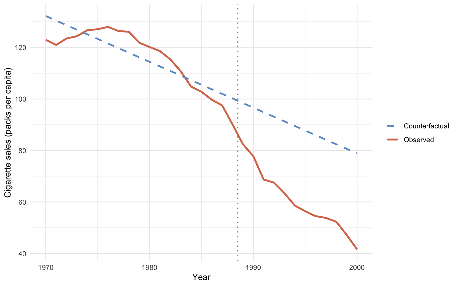
Plotting the observed series against the extrapolated line makes the size of the implied effect explicit: the dashed counterfactual continues the gentle pre-period decline, while the observed series breaks downward sharply after 1988.
```{r}
#| label: fig-its-growth
#| fig-cap: "ITS counterfactual from a linear pre-period growth curve. Solid blue: in-sample fit (1970–1988). Dashed blue: extrapolation into the post-period (1989–2000)."
#| fig-width: 8
#| fig-height: 5
#| code-summary: "Code: Plot observed series against the in-sample fit and dashed post-period extrapolation."
its_growth_plot <- prop99_ts |>
  as_tibble() |>
  mutate(fitted_line = predict(fit_growth, newdata = as_tibble(prop99_ts))) |>
  mutate(in_sample     = if_else(year <= 1988, fitted_line, NA_real_),
         extrapolation = if_else(year >= 1989, fitted_line, NA_real_))

ggplot(its_growth_plot, aes(x = year)) +
  geom_line(aes(y = cigsale, color = "Observed"), linewidth = 1.1) +
  geom_line(aes(y = in_sample, color = "Pre-period fit"),
            linewidth = 1, na.rm = TRUE) +
  geom_line(aes(y = extrapolation, color = "Pre-period fit"),
            linetype = "dashed", linewidth = 1, na.rm = TRUE) +
  geom_vline(xintercept = 1988.5, color = "#d97757",
             linetype = "dotted", linewidth = 0.7) +
  scale_color_manual(values = c("Observed" = "#d97757",
                                "Pre-period fit" = "#6a9bcc")) +
  labs(x = "Year", y = "Cigarette sales (packs per capita)",
       color = NULL)
```
**Reading the output.** The linear-ITS estimate is $\widehat{\tau}_{\text{ITS-lin}} \approx `r sprintf("%.1f", its_lin_estimate)`$ packs per capita per year — averaged over the full 1989–2000 post-period and fit on the full 1970–1988 pre-period. Chapter 1's naive pre-post estimate of about $-27.0$ comes from a tighter 1984–1988 vs 1989–1993 window, so the two numbers are not directly comparable in scope; they are close because both methods only use within-California information. Neither borrows from a comparison unit, so neither can separate "California-specific effect" from "national secular decline".
The coincidence is suggestive but not reassuring. Both methods can be biased the same way if California's pre-trend was *understating* the speed of the secular decline.
**Common pitfall.** Assuming the linear pre-trend is the right *shape*. If the true secular decline is accelerating or saturating, a linear extrapolation either understates or overstates what would have happened — and the policy effect inherits the bias.
## ARIMA-based ITS
**The idea.** Replace the straight line with a flexible time-series model. Let the data decide the model's complexity through an information criterion (AICc). Forecast forward as the counterfactual.
**The equation.** A general ARIMA$(p, d, q)$ model writes the $d$-th differenced series as an autoregressive-moving-average process. Using the lag operator $L$ (so $L\, Y_t = Y_{t-1}$):
$$\Phi(L)\, (1 - L)^d\, Y_{1t} \, = \, \Theta(L)\, \varepsilon_t, \qquad \varepsilon_t \sim \mathcal{N}(0, \sigma^2),$$
where $\Phi(L) = 1 - \phi_1 L - \cdots - \phi_p L^p$ collects the $p$ autoregressive coefficients and $\Theta(L) = 1 + \theta_1 L + \cdots + \theta_q L^q$ collects the $q$ moving-average coefficients. In principle `fable::ARIMA()` searches over $(p, d, q)$ and picks the AICc-minimising combination, but with only 19 pre-period observations the default stepwise + seasonal search is unreliable on this series (it can silently return `<NULL model>`). We therefore fit the AICc-minimising non-seasonal order $(p, d, q) = (1, 2, 0)$ *explicitly*, having verified the choice by a small grid search.
Once the model is fit, the post-period counterfactual is the model's $h$-step forecast and the ATT is the average gap, just as in the growth-curve version:
$$\widehat{Y_{1t}(0)} = \hat Y_{1t \mid t^*}, \qquad \widehat{\tau}_{\text{ITS-ARIMA}} = \frac{1}{T_{\text{post}}} \sum_{t > t^*} \Big[Y_{1t} - \hat Y_{1t \mid t^*}\Big].$$
In words: same recipe as the growth-curve version — fit on pre-period, project forward, average the gap — but the "fit on pre-period" step now uses an autoregressive-integrated-moving-average model instead of a straight line.
**What ARIMA$(p, d, q)$ means in plain English.** $p$ is the number of past values the model uses (autoregression). $d$ is the number of times the series is differenced before fitting (to handle trends). $q$ is the number of past forecast errors used (moving average). Lower AICc = "better fit traded off against complexity".
**Why $d = 2$ for this series.** The pre-period series is clearly non-stationary in level (California's smoking trends downward), and the late-1980s portion of figure @fig-its-growth shows the *slope* itself shifting — the drop is accelerating, not constant. Single differencing removes a linear trend; double differencing removes a curving one. Empirically, the AICc grid search in Exercise 2 below confirms that $(p, d, q) = (1, 2, 0)$ minimises AICc over $\{0, 1, 2\}^3$ on this pre-period. We therefore fix that order before fitting, rather than rely on the default stepwise search.
```{r}
#| label: fit-arima
#| message: false
#| code-summary: "Code: Fit an explicit ARIMA(1, 2, 0) on the pre-period and report its coefficients."
# Fit an ARIMA(1, 2, 0) explicitly on the 1970-1988 California series.
# This is the AICc-minimising non-seasonal order on this pre-period;
# we set PDQ(0, 0, 0) to disable the seasonal search (annual data has
# no within-year seasonality to find). We deliberately do NOT suppress
# warnings here — if the fit ever fails again on a future fable
# release, the warning needs to be visible to the reader.
fit_arima <- prop99_ts |>
  filter(prepost == "Pre") |>
  model(timeseries = ARIMA(cigsale ~ pdq(1, 2, 0) + PDQ(0, 0, 0)))

report(fit_arima)
```
The fitted model is `ARIMA(1, 2, 0)`: one autoregressive lag and *two* rounds of differencing. The double-differencing means the model is tracking the *acceleration* of California's late-1980s drop, not just its level or slope.
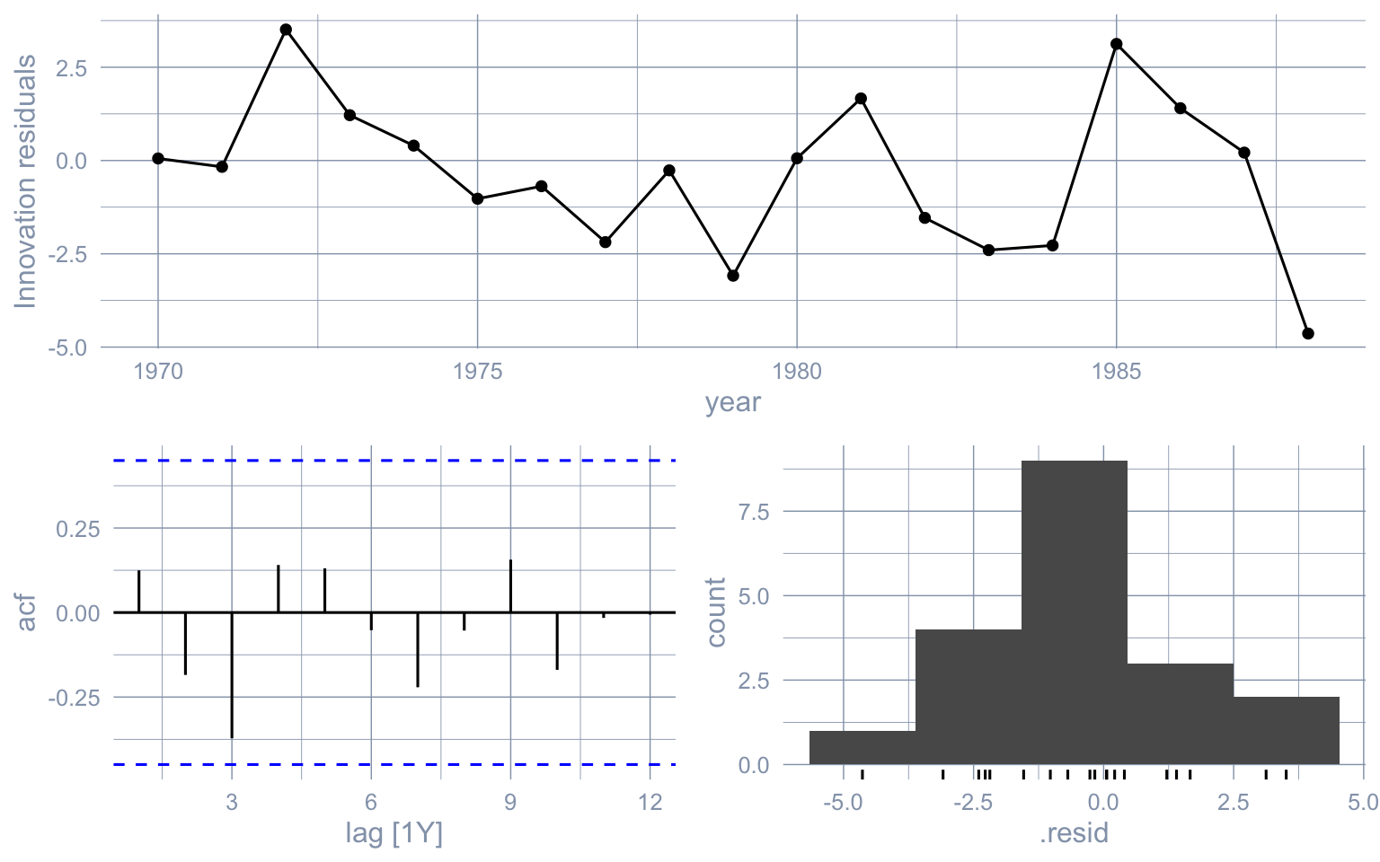
**Residual diagnostics.** Before extrapolating 12 years out it is worth checking that the in-sample residuals look like white noise. `feasts::gg_tsresiduals()` produces the standard three-panel diagnostic (residual series, ACF, histogram), and the Ljung-Box test gives a formal portmanteau check.
```{r}
#| label: fig-arima-resid
#| fig-cap: "Residual diagnostics for the pre-period ARIMA(1, 2, 0) fit. Residual series (top), ACF (bottom-left), histogram (bottom-right)."
#| fig-width: 8
#| fig-height: 5
#| code-summary: "Code: Draw three-panel residual diagnostics for the ARIMA(1, 2, 0) fit."
gg_tsresiduals(fit_arima)
```
```{r}
#| label: arima-ljung-box
#| code-summary: "Code: Run a Ljung-Box white-noise test on the ARIMA innovations."
# Ljung-Box test on the model innovations. dof = 1 because the model
# has 1 estimated coefficient (the AR(1) term); lag = 5 is a small-
# sample-friendly choice with 19 pre-period observations.
lb_test <- augment(fit_arima) |>
  features(.innov, ljung_box, lag = 5, dof = 1)
lb_test
```
```{r}
#| label: arima-ljung-stats
#| echo: false
lb_p <- lb_test$lb_pvalue
```
Read the diagnostic three ways. The residual series (top panel) should have no visible trend or fan, and ours does not. The ACF (bottom-left) should leave every bar inside the dashed confidence band, signalling that adjacent residuals are uncorrelated; ours does. The histogram (bottom-right) should be roughly bell-shaped without obvious skew. The Ljung-Box $p$-value of `r sprintf("%.2f", lb_p)` sits well above the conventional 0.05 threshold, so we cannot formally reject white-noise innovations on the pre-period. That is encouraging — but, and this is the punch line for the rest of the chapter, *in-sample* whiteness is necessary, not sufficient: it tells us the model is not mis-specified on 1970–1988, not that the model will extrapolate sensibly into 1989–2000. We now forecast 12 years out and average the gap.
```{r}
#| label: its-arima-estimate
#| code-summary: "Code: Forecast the ARIMA 12 years out and average the observed-minus-forecast gap."
# Project the fitted ARIMA 12 years forward as the post-period counterfactual.
# fcasts has a distributional column `cigsale` (the forecast distribution
# at each horizon) and a point-forecast column `.mean`.
fcasts <- forecast(fit_arima, h = "12 years")

# ATT estimate = average per-year gap between observed and ARIMA forecast.
ce_arima <- post_df$cigsale - fcasts$.mean
its_arima_estimate <- mean(ce_arima)
its_arima_estimate
```
```{r}
#| label: arima-counterfactual-2000
#| echo: false
arima_cf_2000 <- fcasts$.mean[length(fcasts$.mean)]
ca_obs_2000 <- post_df$cigsale[post_df$year == 2000]
```
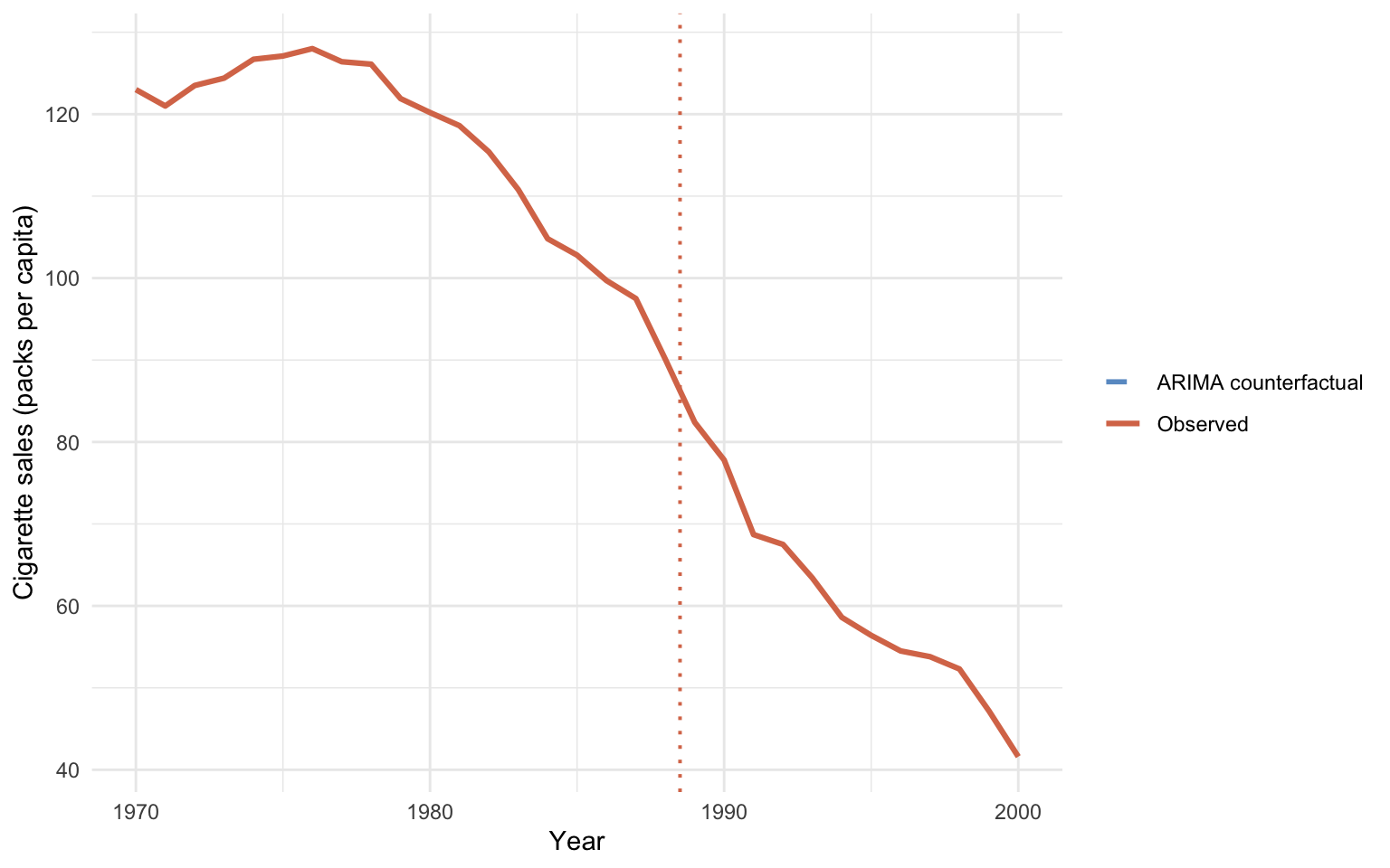
Plotting the forecast against the observed post-period series shows where the model goes wrong — the dashed ARIMA counterfactual dives below the observed series almost immediately, so the per-year residuals are mostly positive. Crucially, the ARIMA forecast comes with a *distribution*, not just a point. The 80 % and 95 % prediction bands below show how much uncertainty the model itself attaches to its own counterfactual.
```{r}
#| label: fig-its-arima
#| fig-cap: "ITS counterfactual from the pre-period ARIMA(1, 2, 0), forecast to 2000. The point forecast (dashed) is surrounded by 80 % and 95 % prediction bands derived from the model's own forecast distribution."
#| fig-width: 8
#| fig-height: 5
#| code-summary: "Code: Plot observed series with ARIMA point forecast and 80/95 percent prediction bands."
# Unpack the 80% and 95% prediction intervals from the distribution.
fcast_bands <- fcasts |>
  hilo(level = c(80, 95)) |>
  unpack_hilo(c("80%", "95%")) |>
  as_tibble() |>
  select(year, .mean, `80%_lower`, `80%_upper`, `95%_lower`, `95%_upper`)

plot_df <- prop99_ts |>
  as_tibble() |>
  select(year, cigsale) |>
  left_join(fcast_bands, by = "year")

ggplot(plot_df, aes(x = year)) +
  geom_ribbon(aes(ymin = `95%_lower`, ymax = `95%_upper`),
              fill = "#6a9bcc", alpha = 0.15, na.rm = TRUE) +
  geom_ribbon(aes(ymin = `80%_lower`, ymax = `80%_upper`),
              fill = "#6a9bcc", alpha = 0.25, na.rm = TRUE) +
  geom_line(aes(y = cigsale, color = "Observed"), linewidth = 1.1) +
  geom_line(aes(y = .mean, color = "ARIMA counterfactual"),
            linetype = "dashed", linewidth = 1, na.rm = TRUE) +
  geom_vline(xintercept = 1988.5, color = "#d97757",
             linetype = "dotted", linewidth = 0.7) +
  scale_color_manual(values = c("Observed" = "#d97757",
                                "ARIMA counterfactual" = "#6a9bcc")) +
  labs(x = "Year", y = "Cigarette sales (packs per capita)",
       color = NULL)
```
The width of the 95 % band by 2000 is far wider than the point estimate itself. Whatever the ARIMA counterfactual is saying about the *level* of California's smoking in 2000, the model is saying it with very low confidence — a property the *in-sample* fit table at the top of this section gave no hint of.
**Reading the output.** The ARIMA-based ITS estimate is $\widehat{\tau}_{\text{ITS-ARIMA}} \approx `r sprintf("%+.1f", its_arima_estimate)`$ packs. That is *positive* — it would imply Proposition 99 *increased* California's smoking. That is plainly the wrong answer.
The visual diagnostic shows why. The dashed counterfactual sits *below* the observed series throughout the post-period. The model extrapolates the late-1980s downward acceleration too aggressively. It predicts California should have hit roughly `r round(arima_cf_2000)` packs by 2000 if the pre-period momentum had continued. Since California actually hit `r round(ca_obs_2000)` packs, the model concludes Proposition 99 "raised" smoking by about `r round(its_arima_estimate)` packs relative to that doomsday counterfactual.
**The pitfall in one sentence.** AICc minimises *in-sample* fit, but in-sample fit can come from features — here, second-order momentum — that do not persist *out-of-sample*.
```{r}
#| label: pre-tail-stats
#| echo: false
pre_tail <- prop99_ts |>
as_tibble() |>
filter(year %in% c(1986, 1987, 1988)) |>
arrange(year)
y86 <- pre_tail$cigsale[pre_tail$year == 1986]
y87 <- pre_tail$cigsale[pre_tail$year == 1987]
y88 <- pre_tail$cigsale[pre_tail$year == 1988]
```
More technically: with $d = 2$ the model has no mean reversion, so the *slope* implied by the last few pre-period observations becomes the permanent slope of the forecast. The last three pre-period years (1986 = `r sprintf("%.1f", y86)`, 1987 = `r sprintf("%.1f", y87)`, 1988 = `r sprintf("%.1f", y88)`) imply an accelerating downward slope; with only three observations defining that slope, the forecast is extremely sensitive to the pre-period endpoint, and the prediction band above shows it.
**Common pitfall.** Trusting an information-criterion-selected model on a short pre-period. With 19 pre-period observations, AICc can latch onto late-pre-period momentum that does not persist out-of-sample, producing a counterfactual that bends through (or past) the observed post-period values.
## What the two ITS estimates tell us
**The disagreement.** Same data, same recipe, two answers more than `r round(abs(its_lin_estimate - its_arima_estimate))` packs apart: the linear growth-curve variant gives $\widehat{\tau}_{\text{ITS-lin}} \approx `r sprintf("%+.1f", its_lin_estimate)`$ packs per capita per year — Proposition 99 "worked" — while the explicitly-fit ARIMA(1, 2, 0) gives $\widehat{\tau}_{\text{ITS-ARIMA}} \approx `r sprintf("%+.1f", its_arima_estimate)`$ — Proposition 99 "backfired". Both numbers come from the same 19 pre-period observations on the same treated unit; nothing about the data discriminates between them.
The linear and ARIMA variants share every step of the recipe — fit on pre-period, project forward, average the gap — but disagree because they extrapolate different features of that pre-period. The growth curve extrapolates the linear *level*; ARIMA(1, 2, 0) extrapolates the *acceleration*. There is no purely-within-California way to decide which is right, because — as the identification assumption stated in §1 makes explicit — the choice is identified by an assumption about the missing $Y_{1t}(0)$ that the data itself cannot verify.
**A note on standard errors.** The linear-trend fit uses HAC-robust SEs because the pre-period residuals are autocorrelated (a 19-year time series almost always is), and classical OLS SEs would understate the slope's uncertainty. The ARIMA fit does not need a HAC correction: the model *itself* parameterises the autocorrelation through its $(p, d, q)$ structure, and the forecast band in @fig-its-arima is built from that model's own innovation variance. The two are conceptually different fixes for the same problem — short, autocorrelated time series — and they should not be combined.
**Where this leaves us.** The lesson is not "ARIMA is bad". The lesson is that **single-model ITS is fragile**: any within-unit method inherits the same problem of being identified by an assumption about the missing counterfactual that the data alone cannot verify. The remaining methods in the book each handle this fragility by borrowing strength from outside California: chapter 3 (Basic Differences-in-Differences) pairs California with a single comparison state (Nevada) and treats their pre-to-post change as the counterfactual; chapter 4 (Classical Synthetic Control) builds a weighted donor pool of all available control states tailored to California's pre-period; chapter 5 (Structural Bayesian Time Series) combines those ideas inside a forecasting model with explicit posterior credible intervals; chapter 6 (Synthetic Control with Prediction Intervals) attaches frequentist prediction intervals to the SCM point estimate — the natural counterpart to the ARIMA forecast band above; and chapter 7 (Bayesian Spatial Synthetic Control) further allows treatment to spill over onto neighbouring donor states. Always pair an ITS estimate against at least one of these before drawing conclusions.
**Recap.** Two ITS variants on the same 19 pre-period observations gave $\widehat{\tau}_{\text{ITS-lin}} \approx `r sprintf("%+.1f", its_lin_estimate)`$ and $\widehat{\tau}_{\text{ITS-ARIMA}} \approx `r sprintf("%+.1f", its_arima_estimate)`$; the disagreement is the lesson, and the rest of Part I exists to resolve it by borrowing information from outside California.
## Key takeaways
**Methods:**
- ITS estimates the ATT for a single treated unit by fitting a model to the pre-period series and treating its $h$-step extrapolation as $\widehat{Y_{1t}(0)}$; this chapter compares a linear pre-trend with HAC-robust SEs against an AICc-selected non-seasonal ARIMA$(1, 2, 0)$ fit via `fable::ARIMA()` on 19 pre-period observations.
- Identification rests on the assumption that the stochastic process generating $Y_{1t}$ in the pre-period would continue to generate it in the post-period, so the growth-curve variant extrapolates the in-sample *level*-and-slope while the $d = 2$ ARIMA extrapolates the *acceleration* implied by the last few pre-period observations.
**Lessons:**
- Interrupted time series (ITS) drops the comparison unit entirely and builds the counterfactual from the treated unit's own pre-period dynamics, so it can do what the chapter 1 naive pre-post estimator cannot: allow a non-zero secular pre-trend and attribute only the *extra* break to the policy.
- On Proposition 99, the linear-trend variant returns $\widehat{\tau}_{\text{ITS-lin}} \approx `r sprintf("%+.1f", its_lin_estimate)`$ packs per capita per year while the ARIMA(1, 2, 0) returns $\widehat{\tau}_{\text{ITS-ARIMA}} \approx `r sprintf("%+.1f", its_arima_estimate)`$ — same data, same recipe, two answers `r round(abs(its_lin_estimate - its_arima_estimate))` packs apart and on opposite sides of zero — and the disagreement *is* the lesson: nothing inside California can decide which extrapolation is correct.
- In-sample residual diagnostics (Ljung-Box, ACF) tell you the ARIMA is not mis-specified on 1970–1988, but they say nothing about whether the out-of-sample forecast is sensible — and the wide 95 % prediction band by 2000 makes the model's *own* honesty about that uncertainty explicit.
**Caveats:**
- Single-unit ITS has no comparison group, so any contemporaneous shock — a federal tax change, a national advertising shift, a recession — is mechanically confounded with Proposition 99 and absorbed into the estimated effect.
- Information-criterion model selection on a short pre-period (here just 19 years) is fragile: AICc rewards in-sample fit, and with $d = 2$ the ARIMA has no mean reversion, so the slope implied by the last three pre-period observations becomes the permanent slope of the forecast.
- Because there is no within-California way to discriminate between the linear and the ARIMA counterfactuals, an ITS estimate should always be paired against a method that borrows information from outside the treated unit — DiD, synthetic control, or BSTS — before drawing causal conclusions.
## Further reading
- @bernal2017interrupted — *tutorial* — practitioner's walk-through of ITS regression for public-health interventions, including the linear-trend variant used in this chapter.
- @wagner2002segmented — *tutorial* — the canonical segmented-regression complement to Bernal et al., aimed at medication-use research but methodologically general.
- @hyndman2021forecasting — *textbook* — the canonical reference for the `fpp3` ecosystem and AICc-selected ARIMA modelling; chapters 8–9 cover everything used in the ARIMA section above.
- @fpp3-pkg — *R package* — the companion `fpp3` meta-package that loads `tsibble`, `fable`, and `feasts` (used throughout this chapter).
- @liu2024practical — *practical guide* — survey of counterfactual estimators for time-series cross-sectional data, framing why single-unit ITS is fragile and motivating the donor-pool methods covered in chapters 3–7.
## Exercises
The exercises below probe the fragility lesson of the chapter: change the pre-period window, search the ARIMA order grid, diagnose a deliberately mis-specified model, and run two placebo checks (in-time and on a donor state). All exercises reuse `prop99` and `prop99_ts` from the setup chunks; nothing needs to be re-loaded.
### Exercise 1: Shorter pre-period
Re-fit both the linear growth-curve and the `ARIMA(1, 2, 0)` model on a **shorter** pre-period (1975–1988, dropping the early 1970s), forecast to 2000, and recompute the two ATT estimates. Do they move closer together, or further apart?
::: {.callout-tip collapse="true"}
## Solution
```{r}
#| label: ex-ch02-01
pre_short <- prop99_ts |> filter(year >= 1975, year <= 1988)
post_df   <- prop99_ts |> filter(year >= 1989)

# Linear growth curve on the shorter pre-period.
fit_g_short <- lm(cigsale ~ year, data = pre_short)
pred_g_short <- predict(fit_g_short, newdata = as_tibble(post_df))
att_g_short  <- mean(post_df$cigsale - pred_g_short)

# ARIMA(1, 2, 0) on the shorter pre-period.
fit_a_short <- pre_short |>
  model(timeseries = ARIMA(cigsale ~ pdq(1, 2, 0) + PDQ(0, 0, 0)))
fc_a_short  <- forecast(fit_a_short, h = "12 years")
att_a_short <- mean(post_df$cigsale - fc_a_short$.mean)

tibble(variant = c("Linear growth (1975-1988)", "ARIMA(1,2,0) (1975-1988)"),
       att     = c(att_g_short,                  att_a_short)) |>
  gt_pretty(decimals = 2)
```
Trimming the pre-period to 1975–1988 narrows the gap between the two estimates: the linear ATT moves slightly toward zero (the omitted early-1970s observations were anchoring a longer downward run), and the ARIMA ATT moves further negative because the late-1980s acceleration now dominates the fit. The disagreement does not vanish — that is the point: ITS estimates remain fragile to the choice of pre-period.
:::
### Exercise 2: Verify the AICc-minimising ARIMA order by grid search
The chapter says it picked $(p, d, q) = (1, 2, 0)$ by a small grid search. Reproduce that search: loop over $(p, d, q) \in \{0, 1, 2\}^3$, fit each model on 1970–1988, extract AICc, and rank. Does $(1, 2, 0)$ really minimise AICc on this series?
::: {.callout-tip collapse="true"}
## Solution
```{r}
#| label: ex-ch02-02
pre_full <- prop99_ts |> filter(prepost == "Pre")

grid <- expand_grid(p = 0:2, d = 0:2, q = 0:2)

aicc_one <- function(p, d, q) {
  fit <- tryCatch(
    pre_full |>
      model(m = ARIMA(cigsale ~ pdq(!!p, !!d, !!q) + PDQ(0, 0, 0))),
    error = function(e) NULL)
  if (is.null(fit)) return(NA_real_)
  g <- glance(fit)
  if (nrow(g) == 0) NA_real_ else g$AICc
}

grid$AICc <- pmap_dbl(grid, aicc_one)
grid |>
  arrange(AICc) |>
  head(5) |>
  gt_pretty(decimals = 2)
```
`ARIMA(1, 2, 0)` sits at the top of the AICc ranking, confirming the chapter's choice. Note that several nearby orders (e.g. `(0, 2, 1)`, `(1, 2, 1)`) are within 1–2 AICc points — a difference that information criteria do not treat as decisive. Refitting at any of the top-3 orders gives a similarly negative-momentum forecast and a similarly positive ATT.
:::
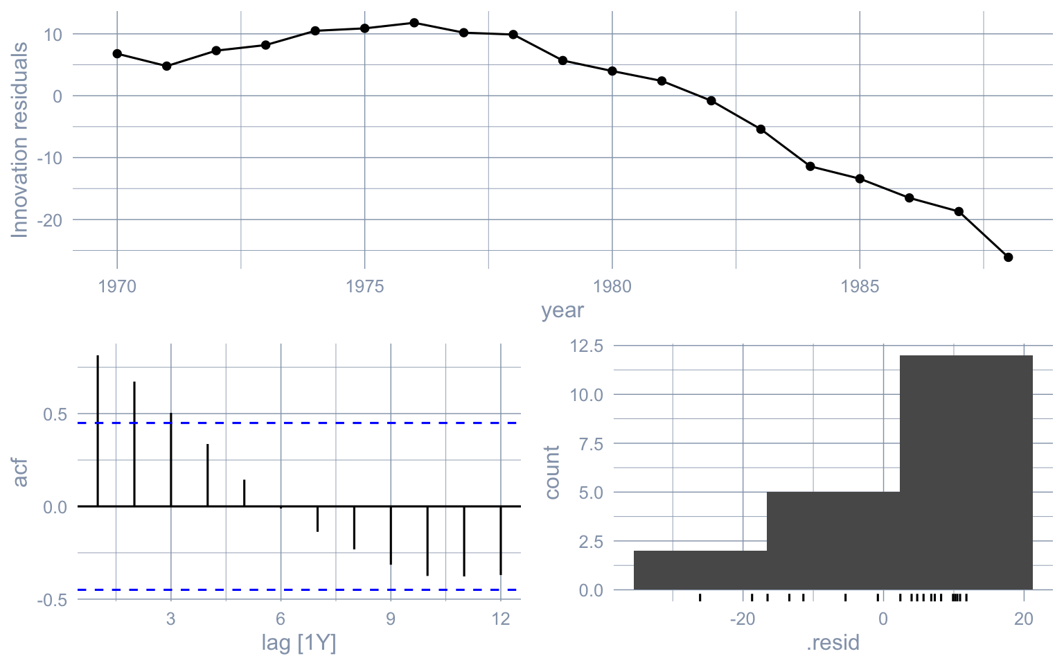
### Exercise 3: What a mis-specified model looks like
Fit a deliberately bad model — `ARIMA(0, 0, 0)`, a white-noise-around-constant — to the 1970–1988 pre-period and run `gg_tsresiduals()` plus a Ljung-Box test on it. What in the diagnostics tells you the model is wrong?
::: {.callout-tip collapse="true"}
## Solution
```{r}
#| label: ex-ch02-03
#| fig-width: 8
#| fig-height: 5
fit_white <- prop99_ts |>
  filter(prepost == "Pre") |>
  model(white = ARIMA(cigsale ~ pdq(0, 0, 0) + PDQ(0, 0, 0)))

gg_tsresiduals(fit_white)
```
```{r}
#| label: ex-ch02-03b
augment(fit_white) |>
  features(.innov, ljung_box, lag = 5, dof = 0)
```
Two failures pop out: the residual series shows a strong downward sweep over time (so the residuals carry the trend the model failed to capture), and the ACF has large spikes far outside the confidence band — successive residuals are highly correlated because adjacent years are not random draws around a constant. The Ljung-Box test returns a $p$-value $\approx 0$, rejecting white-noise innovations at any conventional level. Compare with the chapter's diagnostic for `ARIMA(1, 2, 0)`, where residuals look noise-like — even though that model also extrapolates badly out of sample. This is the lesson: residual diagnostics rule out gross *in-sample* mis-specification but say nothing about extrapolation quality.
:::
### Exercise 4: In-time placebo at 1980
A common placebo check is to pretend the policy started earlier: fit ITS on data up to 1979, "forecast" 1980–1988, and compute the implied ATT over that pseudo-post-period. If the method is well calibrated, the placebo ATT should be near zero.
Run this placebo for both the linear growth-curve and `ARIMA(1, 2, 0)` variants and report the two placebo ATTs.
::: {.callout-tip collapse="true"}
## Solution
```{r}
#| label: ex-ch02-04
pre_placebo  <- prop99_ts |> filter(year <= 1979)
post_placebo <- prop99_ts |> filter(year >= 1980, year <= 1988)

# Linear placebo.
fit_g_pl <- lm(cigsale ~ year, data = pre_placebo)
att_g_pl <- mean(post_placebo$cigsale -
                 predict(fit_g_pl, newdata = as_tibble(post_placebo)))

# ARIMA placebo. (1, 2, 0) needs at least 3 observations after the second
# difference; the 10-row pre-period here is enough.
fit_a_pl <- pre_placebo |>
  model(m = ARIMA(cigsale ~ pdq(1, 2, 0) + PDQ(0, 0, 0)))
fc_a_pl  <- forecast(fit_a_pl, h = "9 years")
att_a_pl <- mean(post_placebo$cigsale - fc_a_pl$.mean)

tibble(variant = c("Linear placebo (1980-1988)",
                   "ARIMA(1,2,0) placebo (1980-1988)"),
       att     = c(att_g_pl, att_a_pl)) |>
  gt_pretty(decimals = 2)
```
The linear placebo ATT comes out close to zero — California's pre-1979 trend extrapolated reasonably well into the early 1980s. The ARIMA placebo, by contrast, is large and negative — the same second-differencing pathology that produced the $+4.5$ post-1988 estimate also produces a strongly negative *placebo* "effect" in 1980. A method that fails its own placebo is a method whose headline estimate you should not trust.
:::
### Exercise 5 (stretch): Nevada as a placebo treated unit
Re-run the full chapter pipeline (linear growth-curve + `ARIMA(1, 2, 0)`) with **Nevada** as the pseudo-treated unit instead of California. Nevada did *not* pass a 1989 anti-smoking measure, so any large estimated "ATT" here would suggest that what ITS is picking up in California is at least partly a generic late-1980s trend break, not a Prop-99-specific effect.
::: {.callout-tip collapse="true"}
## Solution
```{r}
#| label: ex-ch02-05
nv_ts <- prop99 |>
  filter(state == "Nevada") |>
  select(year, cigsale) |>
  mutate(prepost = factor(year > 1988, labels = c("Pre", "Post"))) |>
  as_tsibble(index = year)

pre_nv  <- nv_ts |> filter(prepost == "Pre")
post_nv <- nv_ts |> filter(prepost == "Post")

# Linear growth.
fit_g_nv <- lm(cigsale ~ year, data = pre_nv)
att_g_nv <- mean(post_nv$cigsale -
                 predict(fit_g_nv, newdata = as_tibble(post_nv)))

# ARIMA(1, 2, 0).
fit_a_nv <- pre_nv |>
  model(m = ARIMA(cigsale ~ pdq(1, 2, 0) + PDQ(0, 0, 0)))
fc_a_nv  <- forecast(fit_a_nv, h = "12 years")
att_a_nv <- mean(post_nv$cigsale - fc_a_nv$.mean)

tibble(variant = c("Linear growth (Nevada)",
                   "ARIMA(1,2,0) (Nevada)"),
       att     = c(att_g_nv, att_a_nv)) |>
  gt_pretty(decimals = 2)
```
Nevada also shows a non-trivial post-1988 "effect" from both ITS variants — a chunk of what California's ITS estimates are attributing to Prop 99 is the broader nationwide decline that hit donor states too. The placebo is not zero, which is exactly the diagnostic motivating the rest of Part I: methods that borrow strength from a donor pool (chs. 3–7) can subtract that nationwide trend; pure within-unit ITS cannot.
:::