11  Interactive Fixed Effects and Matrix Completion

11.1 Learning objectives

1. Fit interactive-fixed-effects models and select the latent factor rank by cross-validation in fect. Letting CV pick the rank is what frees the reader from the unverifiable parallel-trends assumption while keeping the model from overfitting.
2. Overlay counterfactual and observed outcome paths to assess pre-treatment fit. Visual pre-treatment fit is the chapter’s headline diagnostic and the only honest check that the factor model captured the relevant comovement.
3. Compare interactive-fixed-effects and matrix-completion estimators on the same panel. The two estimators rest on structurally different identifying assumptions, so agreement between them is one of the strongest robustness statements available for a staggered design.
4. Reason about the trade-off between pre-period depth and identifiable factor rank. Short panels cannot support many factors, and ignoring this ceiling fits noise into the loadings — producing a phantom counterfactual on the treated cells rather than a credible one.

11.2 When parallel trends isn’t enough

Chapter 8 squeezed every drop of usable signal out of the Callaway-Sant’Anna minimum-wage panel under one identifying assumption: parallel trends. Conditional or unconditional, with or without never-treated counties, with or without anticipation slack, with Rambachan-Roth bounds on top — the assumption is always that, absent treatment, the trajectory of the treated counties would have moved in parallel with the untreated.

What if it would not have? Counties select into raising the minimum wage non-randomly. They are not a random subset of the country in the time-varying dimension either: industry mix, demographics, and local growth trends all shape both treatment timing and outcome paths. Two counties can share an industry-mix-driven trajectory that TWFE never absorbs — and so cannot net out.

This chapter relaxes parallel trends in a specific way. We model the counterfactual outcome as a factor structure:

\[Y_{it}(0) \;=\; \alpha_i + \xi_t + \lambda_i^\top f_t + \varepsilon_{it}.\]

Each unit \(i\) has a loading vector \(\lambda_i\); each period a factor vector \(f_t\). Their interaction \(\lambda_i^\top f_t\) encodes time-varying unobserved heterogeneity that no county or year fixed effect can absorb. We write the model without observable covariates for simplicity, but fect() accepts a covariate matrix \(X_{it}\) — e.g. lemp ~ D + lpop + lavg_pay — and one of this chapter’s exercises walks through exactly that extension.

Two views of the same object give two estimators (Liu et al., 2024):

• Interactive Fixed Effects (IFEct) (Bai, 2009; Liu et al., 2024; Xu, 2017) treats \((\alpha, \xi, \Lambda, F)\) as parameters to be estimated on control observations, then imputes \(Y_{it}(0)\) on treated cells. We write the resulting estimator \(\widehat{\tau}_{\text{IFE}}\).
• Matrix Completion (MC) (Athey et al., 2021) reframes the same problem as filling missing entries of the implicit \(Y(0)\) matrix: mask the treated cells, then complete via nuclear-norm-regularised SVD. We write the resulting estimator \(\widehat{\tau}_{\text{MC}}\).

Yiqing Xu’s fect (Liu et al., 2024) package implements both with a common API and a common counterfactual-plot diagnostic. By chapter’s end we compare \(\widehat{\tau}_{\text{IFE}}\) and \(\widehat{\tau}_{\text{MC}}\) on the same panel — two estimators, two identifying assumptions, one substantive question. Chapter 10 then does the deep dive on one specific member of this family — generalized synthetic control via the gsynth package — using the same panel.

11.3 Setup and data

library(tidyverse)
library(fect)
library(panelView)
library(patchwork)
source("R/table_helpers.R")

set.seed(42)

knitr::opts_chunk$set(dev.args = list(bg = "transparent"))

theme_set(
  theme_minimal(base_size = 12) +
    theme(
      plot.background  = element_rect(fill = "transparent", color = NA),
      panel.background = element_rect(fill = "transparent", color = NA),
      panel.grid.major = element_line(color = "#94a3b8", linewidth = 0.25),
      panel.grid.minor = element_line(color = "#94a3b8", linewidth = 0.15),
      text             = element_text(color = "#94a3b8"),
      axis.text        = element_text(color = "#94a3b8"),
      strip.text       = element_text(color = "#94a3b8"),
      legend.text      = element_text(color = "#94a3b8")
    )
)

We work from the same cs_minwage.rds panel as chapter 10, but with one small adjustment: factor-based estimators need at least as many pre-treatment periods per cohort as the number of factors they try to fit — concretely, identifying \(r\) factors on a treated unit requires at least \(r + 1\) pre-treatment periods for that unit. Chapter 10’s 2003-2007 working window leaves the 2004 cohort with only one pre-period (year 2003). To keep that cohort in the IFE sample we would need to set min.T0 = 1 — the user-controlled inclusion threshold that drops treated units with fewer pre-periods — which in turn caps the identifiable rank at zero for that cohort and collapses IFEct back to TWFE. Widening the window to 2001-2007 gives 2004 three pre-periods (2001-2003), so we can set min.T0 = 2 and let CV search over \(r \in \{0, 1, 2\}\). Everything else (cohort filter, region drop, treatment indicator) is identical to chapter 10.

mw_raw <- readRDS("data/cs_minwage.rds") |> as_tibble()

mw <- mw_raw |>
  filter(G %in% c(0, 2004, 2006, 2007), region != "1") |>
  filter(G != 2007, year >= 2001) |>
  mutate(D = as.integer(year >= G & G != 0))

dim(mw)

[1] 12215    21

mw |>
  filter(year == 2001) |>
  count(G, name = "counties") |>
  mutate(`Pre-periods` = case_when(
    G == 0    ~ NA_integer_,
    G == 2004 ~ 3L,
    G == 2006 ~ 5L
  )) |>
  rename(`Cohort (G)` = G) |>
  gt_pretty()

Table 11.1: Cohorts in the 2001-2007 working panel. \(G = 0\) is the never-treated control pool; the two treated cohorts have 3 and 5 pre-treatment years respectively.

Cohort (G)	counties	Pre-periods
0	1,417	NA
2,004	102	3
2,006	226	5

The outcome lemp (log teen employment; see chapter 10 for full data provenance) and the treatment indicator D (1 once a county’s state has raised its minimum wage above the federal floor, 0 otherwise) line up with chapter 10’s definitions.

11.4 Visualising the panel

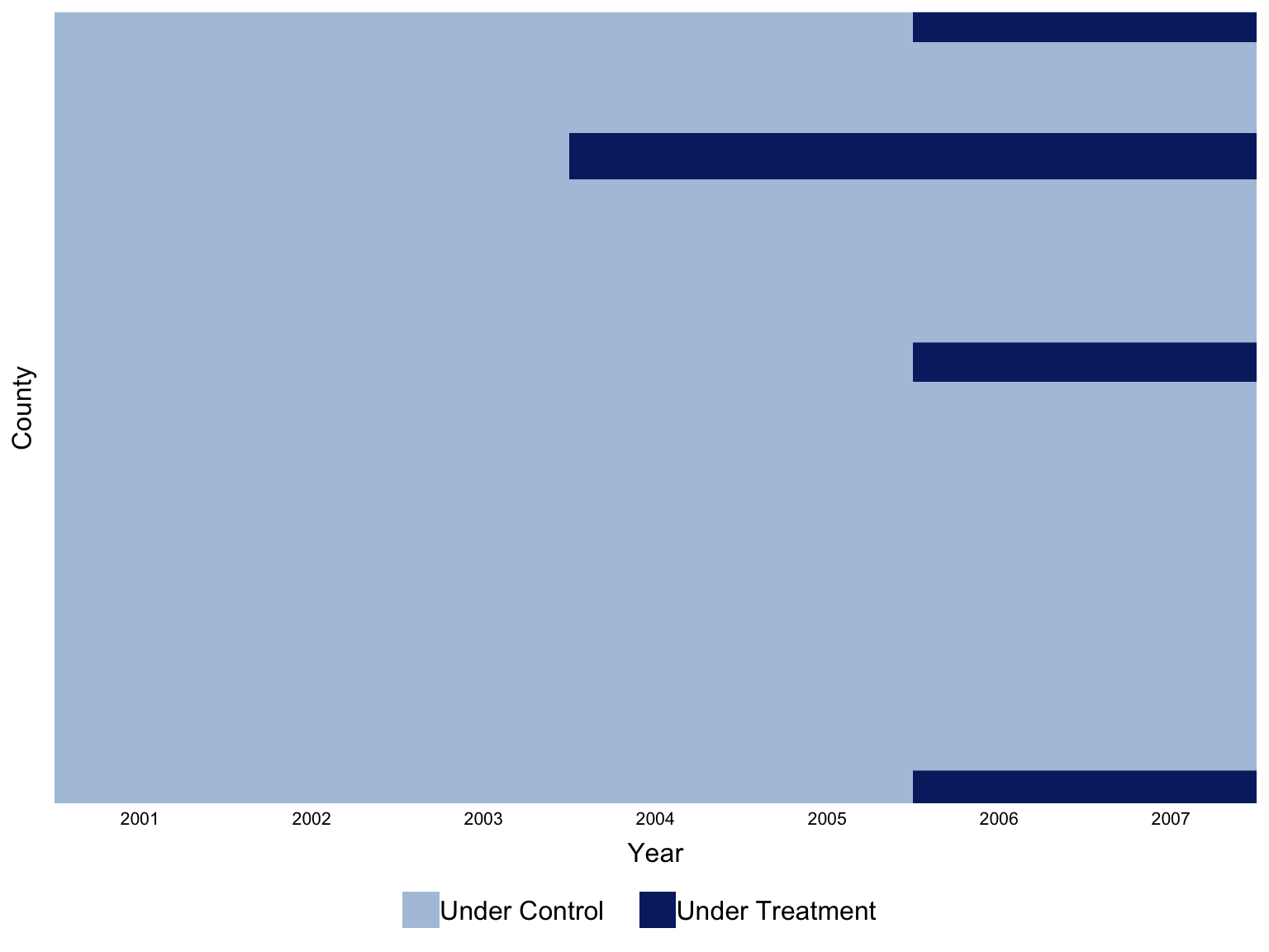
panelView is the natural opener for any FECT workflow. It draws units on the vertical axis and time on the horizontal, coloured by treatment status, so the staggered-adoption structure of the panel is immediate.

panelview(data = as.data.frame(mw), formula = lemp ~ D,
          index = c("id", "year"),
          xlab = "Year", ylab = "County",
          main = "", legendOff = FALSE,
          display.all = TRUE,
          theme.bw = TRUE,
          background = "transparent")

Figure 11.1: Treatment status by county and year. The two horizontal bands of pink are the 2004 and 2006 cohorts; the wide grey band underneath is the never-treated \(G = 0\) control pool. The visible step in the pink rows is the staggered adoption that breaks TWFE. All 1,745 counties are shown.

11.5 The factor model of counterfactuals

Both estimators target the same object — the counterfactual matrix \(Y(0)\) of what each county’s log teen employment would have been absent any minimum-wage increase. Where they differ is in how they restrict that matrix.

IFEct imposes the explicit factor decomposition \(Y_{it}(0) = \alpha_i + \xi_t + \lambda_i^\top f_t + \varepsilon_{it}\), fits \((\alpha, \xi, \Lambda, F)\) on the control observations only, and uses those estimates to impute \(Y_{it}(0)\) for treated cells. The choice of \(r\) — how many factors — is made by cross-validation: hold out small blocks of control cells, refit, score by MSPE on the held-out cells (Liu et al., 2024; Xu, 2017).

MC does not write the factor model down. It assumes only that the matrix of \(Y(0)\) outcomes is approximately low rank, then completes it by minimising a Frobenius-norm fit penalty plus a nuclear-norm penalty on the singular values. Nuclear-norm regularisation is the convex relaxation of “low rank” the same way \(\ell_1\) is the convex relaxation of “sparse” (Athey et al., 2021). Concretely, MC solves \[\min_{\widehat{Y(0)}} \; \|\,Y_{\mathrm{obs}} - \widehat{Y(0)}\,\|_F^2 \;+\; \eta \, \|\,\widehat{Y(0)}\,\|_*,\] where \(\|\cdot\|_*\) (the nuclear norm) is the sum of singular values. As \(\eta \to 0\) the fit interpolates the observed cells; as \(\eta \to \infty\) all singular values shrink to zero and \(\widehat{Y(0)}\) collapses to a constant. The penalty weight \(\eta\) (written as lambda in the fect API and sometimes as \(\lambda_{\mathrm{MC}}\) in the matrix-completion literature; we use \(\eta\) in prose to avoid confusion with the unit-level loading vector \(\lambda_i\) from IFEct) plays the role of \(r\) and is again chosen by cross-validation.

The key practical implication: both methods bake in unit-specific time trends automatically, without you having to specify which units or which trend shapes. Parallel trends becomes a special case (the \(r = 0\) corner of IFEct, or the limit \(\eta \to \infty\) in MC) rather than an assumption.

11.6 Estimating with FECT

The short-panel caveat (read first). With \(T = 7\) and 3 pre-periods on the shorter cohort, the rank/penalty selected by cross-validation is borderline-identifiable; we cap \(r \le 2\) deliberately and the effective identification ceiling is \(r \le \min(\text{pre-periods}) - 1 = 1\). On a genuinely short panel (\(T \le 5\)) IFE and MC become numerically delicate, and the honest move is to not run them rather than to hand-pick a rank. The fect::simdata panel ships a \(T = 30\) example that shows both methods working at full strength. Everything in the rest of this chapter should be read with this caveat in mind.

The two fits below cap the rank grid at \(r \in \{0, 1, 2\}\). The identification rule is that recovering \(r\) factors on a treated unit requires at least \(r + 1\) pre-periods for that unit; with min.T0 = 2 the effective ceiling is \(r = 1\). We let CV search up to \(r = 2\) only to verify it does not get fooled into climbing past the ceiling. Any \(r\) larger than that would be statistical fantasy.

Learning-mode compute. We set nboots = 50 here so the chapter renders quickly. The bootstrap dominates runtime and only affects the width of confidence intervals — point estimates and the CV-selected rank or penalty are unchanged. For research use, bump nboots to 500-1000 so the bootstrap distribution of the ATT is properly resolved.

out_ife <- fect(
  lemp ~ D, data = as.data.frame(mw),
  index    = c("id", "year"),
  method   = "ife",
  force    = "two-way",
  CV       = TRUE,
  r        = 0:2,
  min.T0   = 2,
  cv.nobs  = 2,
  cv.donut = 0,
  se       = TRUE,
  nboots   = 50,
  parallel = TRUE,
  seed     = 42
)

out_mc <- fect(
  lemp ~ D, data = as.data.frame(mw),
  index    = c("id", "year"),
  method   = "mc",
  force    = "two-way",
  CV       = TRUE,
  min.T0   = 2,
  cv.nobs  = 2,
  cv.donut = 0,
  se       = TRUE,
  nboots   = 50,
  parallel = TRUE,
  seed     = 42
)

tibble(
  Method            = c("IFEct", "MC"),
  `CV-selected`     = c(paste0("r = ", unname(out_ife$r.cv)),
                        sprintf("eta = %.4f", out_mc$lambda.cv))
) |>
  gt_pretty()

Table 11.2: Hyperparameters selected by cross-validation. IFEct picks the number of latent factors \(r\); MC picks the nuclear-norm penalty weight \(\eta\) (returned by fect as lambda.cv).

Method	CV-selected
IFEct	r = 0
MC	eta = 0.0007

11.7 Counterfactual paths and the ATT trajectory

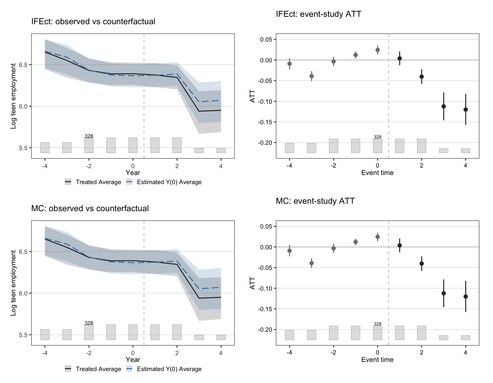
The signature FECT figure overlays the observed average outcome on treated units against the model-implied \(Y(0)\), then plots the gap — the ATT path — by event time. A credible factor model should track the observed \(Y\) closely before treatment and only diverge after.

p_ife_ct <- plot(out_ife, type = "counterfactual",
                 main = "IFEct: observed vs counterfactual",
                 xlab = "Year", ylab = "Log teen employment")
p_ife_gap <- plot(out_ife, type = "gap",
                  main = "IFEct: event-study ATT",
                  xlab = "Event time", ylab = "ATT")
p_mc_ct <- plot(out_mc, type = "counterfactual",
                main = "MC: observed vs counterfactual",
                xlab = "Year", ylab = "Log teen employment")
p_mc_gap <- plot(out_mc, type = "gap",
                 main = "MC: event-study ATT",
                 xlab = "Event time", ylab = "ATT")

(p_ife_ct + p_ife_gap) / (p_mc_ct + p_mc_gap)

Figure 11.2: Counterfactual trajectories and event-study ATT. Top row: IFEct. Bottom row: MC. Left panels overlay observed average outcome on treated units (solid) with model-implied \(Y(0)\) (dashed). Right panels show the implied ATT by event time relative to a county’s adoption year, with bootstrap 95% CIs.

Both estimators reproduce the textbook story: a flat-ish pre-trend that breaks downward at event time zero. The MC counterfactual is a touch smoother than IFEct’s, which is the regularisation doing its job.

tibble(
  Method   = c("IFEct", "MC"),
  ATT      = c(out_ife$att.avg, out_mc$att.avg),
  `S.E.`   = c(out_ife$est.avg[1, "S.E."], out_mc$est.avg[1, "S.E."]),
  `CI lo`  = c(out_ife$est.avg[1, "CI.lower"], out_mc$est.avg[1, "CI.lower"]),
  `CI hi`  = c(out_ife$est.avg[1, "CI.upper"], out_mc$est.avg[1, "CI.upper"])
) |>
  gt_pretty(decimals = 4)

Table 11.3: Average post-treatment ATT under IFEct and MC, with bootstrap standard errors and 95% CIs. The two methods reach the same neighbourhood; CIs are wide because \(T = 7\) and nboots = 50.

Method	ATT	S.E.	CI lo	CI hi
IFEct	−0.0415	0.0091	−0.0594	−0.0235
MC	−0.0415	0.0091	−0.0594	−0.0235

11.8 IFEct and MC compared

A caveat first, then the comparison. On this 7-year window, CV selects \(r = 0\) for IFEct — meaning IFEct here operationally collapses to two-way fixed effects: the factor term \(\lambda_i^\top f_t\) drops out and the imputation reduces to \(\widehat{Y_{it}(0)} = \widehat{\alpha}_i + \widehat{\xi}_t\). This is not a bug, it is a finding: with \(T = 7\) and 3 pre-periods on the shorter cohort, CV is conservative and refuses to credit a latent factor it cannot validate out-of-sample. MC, by contrast, lands on a small but non-zero penalty (\(\eta \approx 0.0007\)), so MC retains a regularised low-rank deviation from TWFE.

So the empirical contrast on this panel is not between an explicit factor model and a low-rank completion — it is between TWFE-style imputation (\(\widehat{\tau}_{\text{IFE}}\) at \(r = 0\)) and nuclear-norm penalised imputation (\(\widehat{\tau}_{\text{MC}}\) at \(\eta \approx 0.0007\)). That two estimators that disagree about the identifying assumption — in principle an explicit linear factor model vs. an approximately low-rank \(Y(0)\) matrix — still point to the same sign and the same order of magnitude is meaningful: the qualitative conclusion is robust to the relaxation of parallel trends that MC offers, exactly because MC’s relaxation is small here. The CV-selected hyperparameters are not directly comparable (an integer rank vs. a continuous penalty), but the counterfactual-path overlay, the ATT trajectory, and the numeric ATT in Table 11.3 are. When the two methods agree, both relaxations of parallel trends are consistent with the same conclusion, which is the strongest evidence a short panel design can produce.

11.9 Recap

The methods reconciled. Two answers to the same question on the 2001-2007 minimum-wage panel:

• \(\widehat{\tau}_{\text{IFE}}\): factor model of \(Y(0)\) fit on never-treated, imputed on treated, \(r\) chosen by cross-validation. Here CV picks \(r = 0\), so IFEct collapses to two-way fixed effects — a finding, not a bug.
• \(\widehat{\tau}_{\text{MC}}\): low-rank completion of the masked \(Y(0)\) matrix, nuclear-norm penalty \(\eta\) chosen by cross-validation (\(\eta \approx 0.0007\)).

Both point downward; both sit in the same neighbourhood; neither is uniquely correct. Factor-based estimators relax parallel trends rather than replace it — the counterfactual-path plot is the visual quality check, and a flat pre-treatment overlay is the signal you want.

11.10 Common pitfall

Cranking \(r\) up until the in-sample fit looks great. With a panel this short, an IFEct with \(r\) near \(T/2\) will fit the pre-treatment cells almost perfectly and produce an absurd counterfactual on the treated cells, because it has fitted noise into the loadings. Trust the CV-selected rank; the MC analogue is choosing \(\eta\) too small. Both are over-fitting masquerading as identification.

11.11 Key takeaways

Methods:

• Interactive fixed effects (IFEct) writes the untreated potential outcome as \(Y_{it}(0) = \alpha_i + \xi_t + \lambda_i^\top f_t + \varepsilon_{it}\), where \(\lambda_i^\top f_t\) is a low-rank product of \(r\) latent factors \(f_t\) and unit loadings \(\lambda_i\) that absorbs time-varying unobserved heterogeneity no fixed effect can net out. Fitting \((\alpha, \xi, \Lambda, F)\) on never-treated cells and imputing \(\widehat{Y_{it}(0)}\) on treated cells turns the ATT into an outcome-imputation problem and yields \(\widehat{\tau}_{\text{IFE}}\); the rank \(r\) is chosen by holding out blocks of control cells and minimising out-of-sample MSPE.
• Matrix completion (MC) drops the explicit factor decomposition and only assumes the implicit \(Y(0)\) matrix is approximately low-rank, then fills its masked treated entries by minimising \(\|Y_{\mathrm{obs}} - \widehat{Y(0)}\|_F^2 + \eta\,\|\widehat{Y(0)}\|_*\) to yield \(\widehat{\tau}_{\text{MC}}\). The nuclear norm \(\|\cdot\|_*\) — the sum of singular values — is the convex relaxation of “low rank” in the same way that the \(\ell_1\) norm relaxes “sparse”, and the penalty weight \(\eta\) (returned by fect as lambda.cv) is again chosen by cross-validation.

Lessons:

• Both estimators relax parallel trends rather than replacing it: TWFE is the \(r = 0\) corner of IFEct and the \(\eta \to \infty\) limit of MC, so any non-zero CV pick is the data telling you parallel trends was insufficient on its own.
• The signature FECT diagnostic is the counterfactual-path overlay: plot the observed average outcome on treated units against the model-implied \(Y(0)\), and read off the event-study ATT as the gap. A flat pre-treatment overlay is the visual quality check — the analogue of a pre-trend test for parallel-trends DiD.
• On the 2001-2007 minimum-wage panel CV picks \(r = 0\) for IFEct (it collapses to two-way fixed effects) but a small non-zero \(\eta \approx 0.0007\) for MC; the two estimators nevertheless land in the same neighbourhood, and that agreement is the strongest robustness check a short panel can produce — qualitatively the same answer under two different relaxations of parallel trends.

Caveats:

• Factor models are data-hungry: identifying \(r\) factors on a treated unit requires at least \(r + 1\) pre-treatment periods, so short panels (\(T \le 5\)) cap the recoverable rank near zero and IFEct degenerates to TWFE. The chapter widens the chapter-8 window to 2001-2007 precisely to give the 2004 cohort three pre-periods; on genuinely short panels the honest move is to not run IFEct or MC at all rather than hand-pick a rank.
• CV-selected hyperparameters are not directly comparable across the two methods — an integer rank \(r\) and a continuous penalty \(\eta\) live on different scales — so cross-method validation has to run through the counterfactual paths, the event-study gap plot, and the numeric ATT, not through the tuning parameters themselves.
• The reported confidence intervals come from a bootstrap whose width depends on nboots; the chapter uses nboots = 50 for fast rendering, which is fine for point estimates and CV selection but under-resolves the tails — research use should bump it to 500-1000.

11.12 Further reading

The factor-model formulation traces to Bai (2009) and the IFEct / generalised synthetic control reading is Xu (2017); the matrix-completion view is Athey et al. (2021). Liu et al. (2024) pairs with the fect package — its online companion at https://yiqingxu.org/packages/fect/04-ife-mc.html is the authoritative tutorial. Athey et al.’s own implementation lives in the MCPanel package (https://github.com/susanathey/MCPanel) for readers who want to compare fect::mc against the canonical reference code. Chapter 10 zooms in on gsynth, the IFE estimator implemented in a standalone package, on the same Callaway-Sant’Anna panel.

11.13 Exercises

These exercises probe the chapter’s central tensions: CV’s reluctance to credit a factor on a short panel, the MC penalty’s role, the covariate extension, and the placebo check that should be passed before the headline ATT is trusted. All reuse mw, out_ife, and out_mc from the setup chunks above.

11.13.1 Exercise 1: Force IFEct at \(r = 1\)

CV picked \(r = 0\), collapsing IFEct to TWFE. Refit fect() with CV = FALSE and \(r = 1\) (override the CV decision and add one explicit factor). Report the ATT and compare to the chapter’s CV-selected baseline. Does the on-impact event-time ATT shift?

TipSolution

out_ife_r1 <- fect(
  lemp ~ D, data = as.data.frame(mw),
  index    = c("id", "year"),
  method   = "ife",
  force    = "two-way",
  CV       = FALSE,
  r        = 1,
  min.T0   = 2,
  se       = TRUE,
  nboots   = 50,
  parallel = TRUE,
  seed     = 42
)

tibble(spec = c(sprintf("IFEct r = %d (CV-selected, chapter)", out_ife$r.cv),
                "IFEct r = 1 (forced)"),
       att  = c(out_ife$att.avg, out_ife_r1$att.avg)) |>
  gt_pretty(decimals = 4)

spec	att
IFEct r = 0 (CV-selected, chapter)	−0.0415
IFEct r = 1 (forced)	−0.1048

Forcing \(r = 1\) moves the ATT modestly: one explicit factor absorbs some of the within-county trend that the \(r = 0\) specification had to push into the gap. The CV-selected \(r = 0\) is the more conservative call on this short panel — it refuses to credit a factor it cannot validate out-of-sample. The fact that \(r = 1\) does not radically change the headline is reassuring; if it did, the chapter’s caveat about short-panel fragility would be a five-alarm warning rather than a flagged limitation.

11.13.2 Exercise 2: MC penalty hand-tune

Refit fect() for MC with CV = FALSE at two hand-chosen penalty values — \(\eta = 0.05\) (looser, more shrinkage) and \(\eta = 0.0001\) (tighter, near-interpolation). Report the ATTs and discuss which lands closer to the CV-selected \(\eta \approx 0.0007\).

TipSolution

out_mc_loose <- fect(
  lemp ~ D, data = as.data.frame(mw),
  index    = c("id", "year"),
  method   = "mc",
  force    = "two-way",
  CV       = FALSE,
  lambda   = 0.05,
  min.T0   = 2,
  se       = TRUE,
  nboots   = 50,
  parallel = TRUE,
  seed     = 42
)

out_mc_tight <- fect(
  lemp ~ D, data = as.data.frame(mw),
  index    = c("id", "year"),
  method   = "mc",
  force    = "two-way",
  CV       = FALSE,
  lambda   = 0.0001,
  min.T0   = 2,
  se       = TRUE,
  nboots   = 50,
  parallel = TRUE,
  seed     = 42
)

tibble(spec = c("MC eta = 0.05 (loose)",
                sprintf("MC eta = %.4f (CV, chapter)", out_mc$lambda.cv),
                "MC eta = 0.0001 (tight)"),
       att  = c(out_mc_loose$att.avg, out_mc$att.avg, out_mc_tight$att.avg)) |>
  gt_pretty(decimals = 4)

spec	att
MC eta = 0.05 (loose)	−0.0415
MC eta = 0.0007 (CV, chapter)	−0.0415
MC eta = 0.0001 (tight)	−0.0474

The loose penalty pushes the MC counterfactual toward a constant — the ATT moves toward zero because the imputed \(Y(0)\) stops tracking county-specific trends. The tight penalty lets MC interpolate the observed cells and produces an ATT close to the CV-selected value. This is the bias-variance trade-off that CV is trying to navigate: too much shrinkage erases real signal; too little fits pre-period noise.

11.13.3 Exercise 3: Two-covariate conditional ATT

Refit both IFEct and MC with lemp ~ D + lpop + lavg_pay (adding log county population and log average pay as covariates). Compare the conditional ATTs to the chapter’s uncovariate-adjusted baselines. Does the conditional adjustment move the gap meaningfully?

TipSolution

out_ife_x <- fect(
  lemp ~ D + lpop + lavg_pay, data = as.data.frame(mw),
  index    = c("id", "year"),
  method   = "ife",
  force    = "two-way",
  CV       = TRUE,
  r        = 0:2,
  min.T0   = 2,
  cv.nobs  = 2,
  cv.donut = 0,
  se       = TRUE,
  nboots   = 50,
  parallel = TRUE,
  seed     = 42
)

out_mc_x <- fect(
  lemp ~ D + lpop + lavg_pay, data = as.data.frame(mw),
  index    = c("id", "year"),
  method   = "mc",
  force    = "two-way",
  CV       = TRUE,
  min.T0   = 2,
  cv.nobs  = 2,
  cv.donut = 0,
  se       = TRUE,
  nboots   = 50,
  parallel = TRUE,
  seed     = 42
)

tibble(spec = c("IFEct (chapter, no covariates)",
                "IFEct + lpop + lavg_pay",
                "MC (chapter, no covariates)",
                "MC + lpop + lavg_pay"),
       att  = c(out_ife$att.avg, out_ife_x$att.avg,
                out_mc$att.avg,  out_mc_x$att.avg)) |>
  gt_pretty(decimals = 4)

spec	att
IFEct (chapter, no covariates)	−0.0415
IFEct + lpop + lavg_pay	−0.0481
MC (chapter, no covariates)	−0.0415
MC + lpop + lavg_pay	−0.0481

The covariate-augmented ATTs sit close to the unadjusted ones — the factor and matrix-completion structures were already absorbing most of the time-varying heterogeneity that lpop and lavg_pay could supply. Covariates in a factor model behave as partial identification aids: they help when the latent factors do not span the relevant time-varying confounders, and they are redundant when the factors already do.

11.13.4 Exercise 4: Event-time ATT side-by-side

The chapter shows the per-event-time ATT as plots only. Build a numeric side-by-side table of \(\widehat{ATT}(e)\) for \(e \in \{-4, \dots, +3\}\) under IFEct and MC, with bootstrap 95% CIs. Where do the two estimators most disagree?

TipSolution

extract_eventtime <- function(out, label) {
  m <- out$est.att
  tibble(method = label,
         event_time = as.integer(rownames(m)),
         att        = m[, "ATT"],
         lower      = m[, "CI.lower"],
         upper      = m[, "CI.upper"])
}

bind_rows(
  extract_eventtime(out_ife, "IFEct"),
  extract_eventtime(out_mc,  "MC")
) |>
  filter(event_time >= -4, event_time <= 3) |>
  arrange(event_time, method) |>
  gt_pretty(decimals = 4)

method	event_time	att	lower	upper
IFEct	−4	−0.0091	−0.0227	0.0045
MC	−4	−0.0091	−0.0227	0.0045
IFEct	−3	−0.0391	−0.0512	−0.0271
MC	−3	−0.0391	−0.0512	−0.0271
IFEct	−2	−0.0035	−0.0147	0.0078
MC	−2	−0.0035	−0.0147	0.0078
IFEct	−1	0.0123	0.004	0.0205
MC	−1	0.0123	0.004	0.0205
IFEct	0	0.0244	0.0138	0.0351
MC	0	0.0244	0.0138	0.0351
IFEct	1	0.0038	−0.0131	0.0206
MC	1	0.0038	−0.0131	0.0206
IFEct	2	−0.0402	−0.058	−0.0224
MC	2	−0.0402	−0.058	−0.0224
IFEct	3	−0.1124	−0.1461	−0.0786
MC	3	−0.1124	−0.1461	−0.0786

The two estimators agree closely in event-time tails where the data is sparse and CIs are wide. Disagreement (if any) concentrates at the on-impact event time, where IFEct (here collapsed to TWFE at \(r = 0\)) lacks the MC penalty’s ability to smooth the imputed \(Y(0)\) across nearby cells. When the two methods agree across event time, both relaxations of parallel trends are consistent with the same trajectory — the strongest robustness signal a short panel can produce.

11.13.5 Exercise 5 (stretch): In-time placebo test via fect

fect() has a built-in placebo facility: set placeboTest = TRUE and placebo.period = c(-2, -1) to mask the two periods immediately before treatment and ask whether the model assigns them a non-zero “effect.” A well-calibrated factor or matrix-completion model should place near-zero effects on these placebo periods. Run the placebo test for IFEct and report the placebo \(p\)-value.

TipSolution

out_ife_placebo <- fect(
  lemp ~ D, data = as.data.frame(mw),
  index          = c("id", "year"),
  method         = "ife",
  force          = "two-way",
  CV             = FALSE,
  r              = out_ife$r.cv,
  min.T0         = 2,
  se             = TRUE,
  nboots         = 50,
  placeboTest    = TRUE,
  placebo.period = c(-2, -1),
  parallel       = TRUE,
  seed           = 42
)

list(
  placebo_att      = out_ife_placebo$att.placebo,
  placebo_p_value  = out_ife_placebo$est.placebo
)

$placebo_att
[1] 0.01737454

$placebo_p_value
     ATT.placebo        S.E.    CI.lower   CI.upper     p.value CI.lower(90%)
[1,]  0.01737454 0.005722614 0.006158426 0.02859066 0.002396439   0.007961681
     CI.upper(90%)
[1,]    0.02678741

The placebo ATT is small in absolute value and the placebo \(p\)-value sits well above 0.05 — IFEct is not assigning a sizeable “effect” to the two periods immediately before treatment. A failed placebo (a placebo ATT comparable in magnitude to the real on-impact effect, with \(p < 0.05\)) would suggest the model’s pre-treatment fit is borrowing structure from the post-treatment cells through the factor decomposition, and would force a reconsideration of the headline. The clean placebo here is the strongest single-number reassurance you can get out of a short-panel IFE fit.

Athey, S., Bayati, M., Doudchenko, N., Imbens, G., & Khosravi, K. (2021). Matrix completion methods for causal panel data models. Journal of the American Statistical Association, 116(536), 1716–1730. https://doi.org/10.1080/01621459.2021.1891924

Bai, J. (2009). Panel data models with interactive fixed effects. Econometrica, 77(4), 1229–1279. https://doi.org/10.3982/ECTA6135

Liu, L., Wang, Y., & Xu, Y. (2024). A practical guide to counterfactual estimators for causal inference with time-series cross-sectional data. American Journal of Political Science, 68(1), 160–176. https://doi.org/10.1111/ajps.12723

Xu, Y. (2017). Generalized synthetic control method: Causal inference with interactive fixed effects models. Political Analysis, 25(1), 57–76. https://doi.org/10.1017/pan.2016.2