---
title: "Generalized Synthetic Control"
---
## Where gsynth fits
Earlier chapters have asked the same counterfactual question in
different ways. Chapter 5 (classical SCM) hand-built a weighted
donor average for a single treated unit. Chapter 7 layered a
spatial prior on top. Chapter 9 abandoned the single-treated-unit
framing entirely and aggregated group-time ATTs under a
parallel-trends assumption. Chapter 10 (when read in sequence)
introduces the interactive-fixed-effects family through `fect`;
this chapter does the focused walkthrough of one specific
estimator in that family — **generalized synthetic control
(gsynth)** [@xu2017generalized] — using the standalone `gsynth`
package on the same Callaway-Sant'Anna minimum-wage panel as
chapter 9.
gsynth sits at the intersection of SCM and panel DiD. Like SCM, it
imputes a counterfactual outcome path for each treated unit using
only never-treated controls. Like staggered DiD, it accommodates
many treated units adopting at different times. The way it threads
that needle is by fitting an **interactive fixed effects** (IFE)
model on the never-treated panel,
$$Y_{it}(0) = \alpha_i + \xi_t + \lambda_i' f_t + X_{it}'\beta +
\varepsilon_{it},$$
then projecting each treated unit onto the estimated factor space
to impute its $Y_{it}(0)$ in the post-treatment period. The
headline ATT is the average gap between observed treated outcomes
and these imputed counterfactuals.
The identifying assumption is **parallel factors**, not parallel
trends: unobserved shocks affecting treated and never-treated units
must load on the same low-rank factor structure $f_t$. When that
holds, gsynth recovers a valid ATT even if the trends themselves
are not parallel. When it does not, the model is misspecified and
the headline ATT is biased — diagnostics matter.
One difference from chapter 9: that chapter truncated the window to
`year >= 2003`, which left cohort 2004 with only one pre-treatment
year. gsynth needs more pre-period to identify factors, so we keep
the full 2001-2007 window. Cohort 2006 then has five pre-treatment
years (2001-2005); cohort 2004 has three (2001-2003). We set
`min.T0 = 3` to admit both cohorts.
## Setup and data
```{r}
#| label: setup
#| message: false
#| warning: false
library(tidyverse)
library(gsynth)
library(panelView)
source("R/table_helpers.R")

set.seed(42)

knitr::opts_chunk$set(dev.args = list(bg = "transparent"))

theme_set(
  theme_minimal(base_size = 12) +
    theme(
      plot.background  = element_rect(fill = "transparent", color = NA),
      panel.background = element_rect(fill = "transparent", color = NA),
      panel.grid.major = element_line(color = "#94a3b8", linewidth = 0.25),
      panel.grid.minor = element_line(color = "#94a3b8", linewidth = 0.15),
      text             = element_text(color = "#94a3b8"),
      axis.text        = element_text(color = "#94a3b8"),
      strip.text       = element_text(color = "#94a3b8"),
      legend.text      = element_text(color = "#94a3b8")
    )
)
```
The dataset ships as `data/cs_minwage.rds` in the chapter bundle.
We restrict to cohorts $G \in \{0, 2004, 2006\}$ and drop the
Northeast region (`region == "1"`) for comparability with
chapter 9. `gsynth()` expects a base `data.frame` — passing a
tibble silently breaks its internal indexing — so we cast with
`as.data.frame()`.
```{r}
#| label: data-load
mw_raw <- readRDS("data/cs_minwage.rds") |> as_tibble()

mw <- mw_raw |>
  filter(G %in% c(0, 2004, 2006), region != "1") |>
  mutate(treat = as.integer(year >= G & G != 0))

mw_df <- as.data.frame(mw)
dim(mw_df)
```
The panel has `r nrow(mw_df)` rows on
`r length(unique(mw_df$id))` counties, balanced across 2001-2007.
The 0/1 indicator `treat` is the only variable gsynth needs to know
about treatment status — its name is deliberately different from
chapter 9's `post` to remind us that gsynth's identification is not
the same as chapter 9's.
```{r}
#| label: tbl-cohort-counts
#| tbl-cap: "Cohort sizes after restriction. G = 0 is the never-treated control pool; cohorts 2004 and 2006 are the staggered treated groups, with 3 and 5 pre-treatment years respectively."
mw_df |>
  filter(year == 2001) |>
  count(G, name = "counties") |>
  mutate(`Pre-treatment years` = ifelse(G == 0, NA_integer_, G - 2001L)) |>
  rename(`Treatment cohort (G)` = G) |>
  gt_pretty()
```
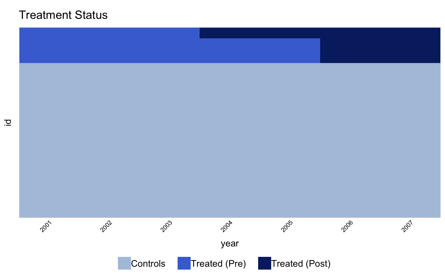
## Treatment timing
The first thing to do with any panel-treatment design is *look at
it*. `panelView` is the package companion to `gsynth`; it produces
a treatment-status heatmap and an outcome-trajectory facet that
together expose anything weird in the data before estimation.
```{r}
#| label: fig-panelview-status
#| fig-cap: "Treatment status heatmap. Rows are counties (grouped by treatment cohort); columns are years. Pink cells are treated; blue cells are control. Within each treated cohort, the pink block starts in the cohort's adoption year. Never-treated counties (G = 0) stay blue throughout."
#| fig-width: 8
#| fig-height: 5
#| message: false
#| warning: false
panelview(lemp ~ treat, data = mw_df,
          index = c("id", "year"),
          pre.post = TRUE,
          by.timing = TRUE,
          display.all = TRUE,
          axis.lab = "time",
          axis.adjust = TRUE)
```
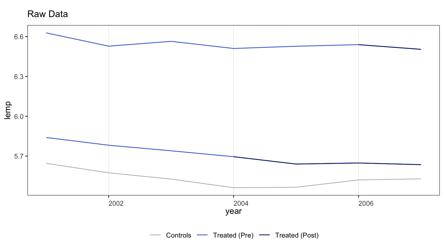
```{r}
#| label: fig-panelview-outcome
#| fig-cap: "Outcome trajectories by cohort. Each thin grey line is one county's log teen employment over time; thick colored lines are cohort means. The pre-treatment trajectories look broadly parallel across cohorts, but with enough texture that a low-rank factor model has something to estimate."
#| fig-width: 8
#| fig-height: 4.5
#| message: false
#| warning: false
panelview(lemp ~ treat, data = mw_df,
          index = c("id", "year"),
          type = "outcome",
          by.cohort = TRUE,
          theme.bw = TRUE)
```
## Baseline: gsynth without factors
The first fit forces $r = 0$ — no latent factors. With two-way
fixed effects (`force = "two-way"`) and no factors, this is the
closest gsynth analogue to the TWFE regression in chapter 9. We
set `min.T0 = 3` so cohort 2004 (which has only 3 pre-treatment
years) isn't dropped, and disable cross-validation (`CV = FALSE`):
gsynth's default rolling-window CV needs `min.T0 + cv.nobs = 8`
pre-treatment periods per treated cohort, which cohort 2004 does
not have. We pick $r$ manually by IC in the next section.
```{r}
#| label: fit-no-factors
#| message: false
#| warning: false
#| cache: true
out_r0 <- gsynth(lemp ~ treat + lpop + lavg_pay,
                 data = mw_df,
                 index = c("id", "year"),
                 force = "two-way",
                 CV = FALSE, r = 0,
                 se = TRUE,
                 inference = "nonparametric",
                 nboots = 500,
                 min.T0 = 3,
                 parallel = TRUE,
                 seed = 42)
```
```{r}
#| label: tbl-baseline
#| tbl-cap: "Overall ATT under gsynth with no factors (r = 0). The point estimate is in the same neighborhood as chapter 9's TWFE coefficient (−0.038), as expected: with no factors, gsynth reduces to a within-transformation panel estimator."
tibble(
  Specification = "gsynth, r = 0 (no factors)",
  Estimate      = out_r0$att.avg,
  `S.E.`        = out_r0$est.avg[1, "S.E."],
  `CI lower`    = out_r0$est.avg[1, "CI.lower"],
  `CI upper`    = out_r0$est.avg[1, "CI.upper"],
  `p-value`     = out_r0$est.avg[1, "p.value"]
) |> gt_pretty(decimals = 4)
```
This baseline is a sanity check: gsynth with no factors should
recover something close to TWFE, and it does. The next step is to
let the model use the never-treated panel to estimate latent
factors and see whether the estimate moves.
## Information criterion across factor counts
The principled way to pick the number of factors $r$ is to fit the
model at several candidate values and select the $r^*$ that
minimises an information criterion. `gsynth` reports both a
[@bai2003inferential]-style IC and a PC criterion; either is a
valid target. We fit $r \in \{0, 1, 2\}$ explicitly — beyond 2 the
panel does not have enough pre-treatment depth to estimate
additional factors.
```{r}
#| label: fit-factor-grid
#| message: false
#| warning: false
#| cache: true
fit_grid <- map(0:2, function(r_val) {
  gsynth(lemp ~ treat + lpop + lavg_pay,
         data = mw_df,
         index = c("id", "year"),
         force = "two-way",
         CV = FALSE, r = r_val,
         se = TRUE,
         inference = "nonparametric",
         nboots = 500,
         min.T0 = 3,
         parallel = TRUE,
         seed = 42)
})
names(fit_grid) <- paste0("r=", 0:2)
```
```{r}
#| label: tbl-ic-grid
#| tbl-cap: "Information criterion and ATT across candidate factor counts. As $r$ grows, in-sample $\\sigma^2$ falls but the model's information cost rises, and IC pushes back. The standard error column tells the rest of the story: at $r = 2$ the SE explodes by two orders of magnitude — a clear sign that fitting two factors leaves too few degrees of freedom in a panel this short."
ic_tbl <- map_dfr(seq_along(fit_grid), function(i) {
  o <- fit_grid[[i]]
  tibble(
    r       = i - 1L,
    ATT     = o$att.avg,
    `S.E.`  = o$est.avg[1, "S.E."],
    IC      = o$IC,
    sigma2  = o$sigma2
  )
})

gt_pretty(ic_tbl, decimals = 4)
```
```{r}
#| label: select-best
candidate <- ic_tbl |> filter(r >= 1)
r_star    <- candidate$r[ which.min(candidate$IC) ]
out       <- fit_grid[[ paste0("r=", r_star) ]]
```
Read literally, the IC table's global minimum is at $r = 0$ — but
that fit *is* the baseline we just produced; calling it the
"factor-model fit" would mean reporting a zero-factor model. We
want to put the factor structure on stage, so we restrict the
selection to $r \ge 1$ and pick the IC-minimising rank from that
subset. That gives $r^* = `r r_star`$, with an ATT roughly twice
the size of the no-factor baseline and a standard error still in
a usable range.
For the rest of the chapter we work with the $r = r^*$ fit.
## Standard gsynth plots
`gsynth::plot()` is the workhorse visualization. Four `type=`
options cover the diagnostic menu the source tutorial demonstrates.
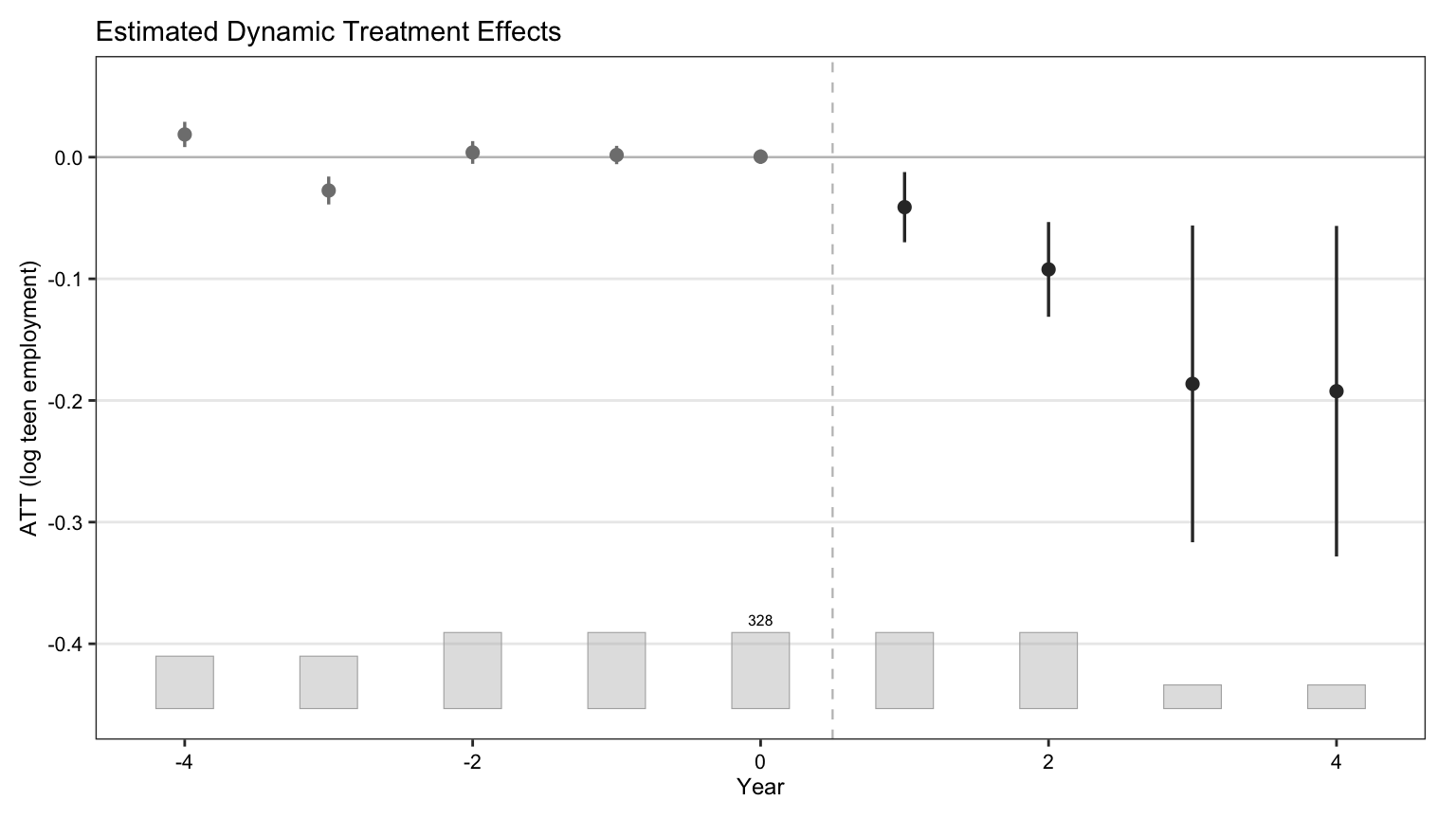
### Gap plot (period-by-period ATT)
```{r}
#| label: fig-gsynth-gap
#| fig-cap: "Period-by-period ATT with 95% nonparametric-bootstrap confidence bands. Pre-treatment periods should hover near zero if the factor model is doing its job; post-treatment effects are the ATT trajectory the chapter is after."
#| fig-width: 8
#| fig-height: 4.5
#| message: false
#| warning: false
plot(out, type = "gap",
     xlab = "Year", ylab = "ATT (log teen employment)",
     main = NULL)
```
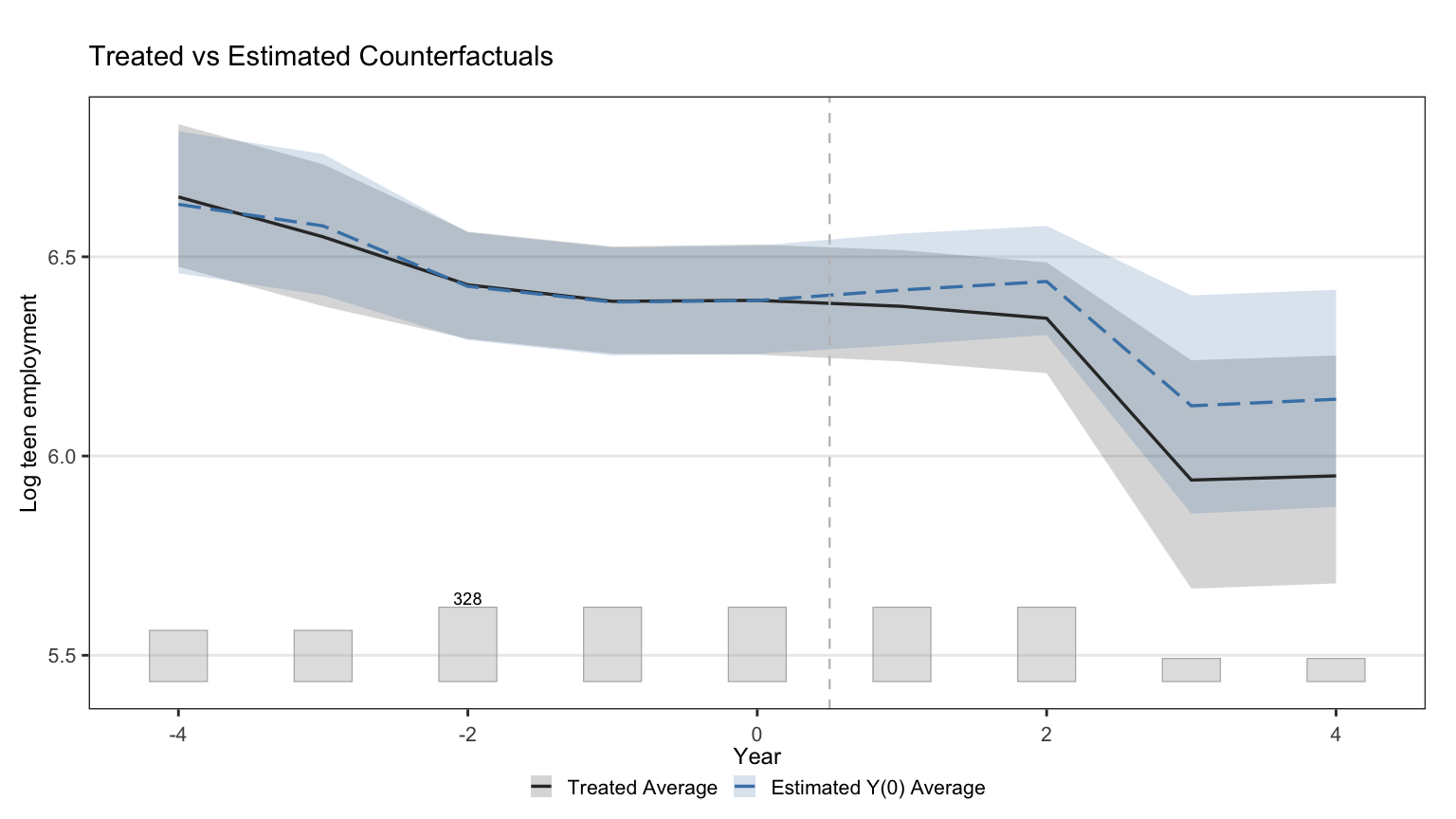
### Counterfactual plot
```{r}
#| label: fig-gsynth-counterfactual
#| fig-cap: "Observed treated-unit outcomes against gsynth's imputed counterfactual. Close tracking before treatment is the visual analogue of the small pre-treatment ATTs in the gap plot."
#| fig-width: 8
#| fig-height: 4.5
#| message: false
#| warning: false
plot(out, type = "counterfactual", raw = "none",
     main = NULL,
     xlab = "Year", ylab = "Log teen employment")
```
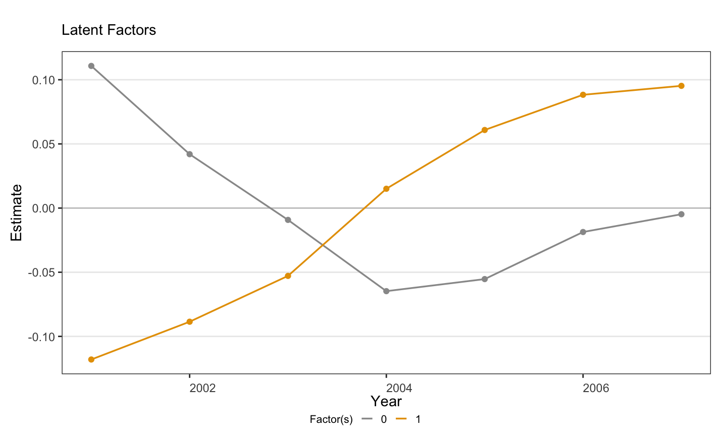
### Estimated factors
```{r}
#| label: fig-gsynth-factors
#| fig-cap: "Estimated latent factor(s) $f_t$ over time. With $r^* = 1$ a single curve is shown; its shape captures the unobserved time-varying shock the factor model is using to explain co-movement in the never-treated panel."
#| fig-width: 7.5
#| fig-height: 4.5
#| message: false
#| warning: false
if (r_star >= 1) {
  plot(out, type = "factors", main = NULL, xlab = "Year")
} else {
  message("No factors to plot (r* = 0).")
}
```
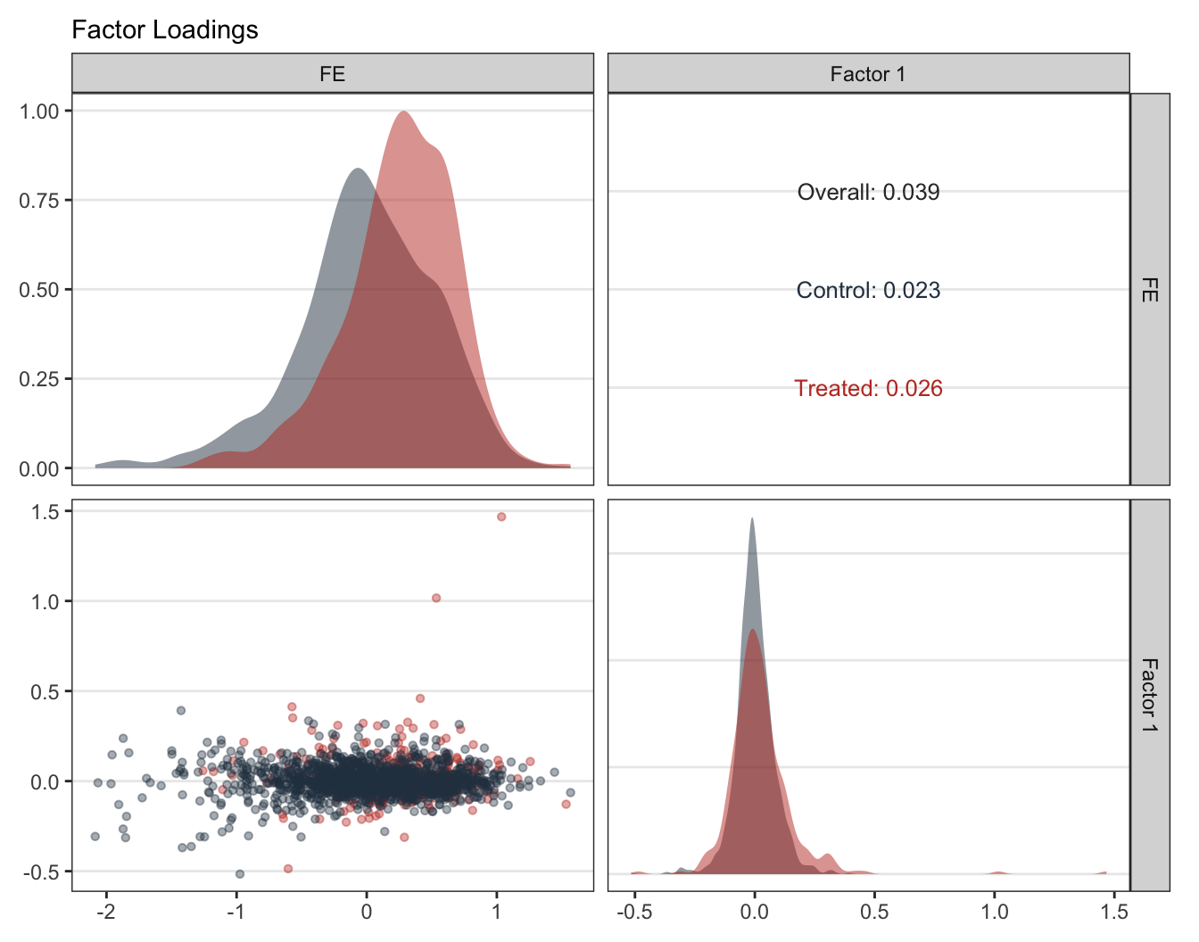
### Factor loadings
```{r}
#| label: fig-gsynth-loadings
#| fig-cap: "Factor loadings $\\lambda_i$ for treated and control counties. Concentration of treated loadings inside the cloud of control loadings is what the gsynth identification needs — it means each treated unit's counterfactual can be expressed as a combination of observed controls rather than an extrapolation."
#| fig-width: 7
#| fig-height: 5.5
#| message: false
#| warning: false
if (r_star >= 1) {
  plot(out, type = "loadings", main = NULL)
} else {
  message("No loadings to plot (r* = 0).")
}
```
## Implied donor weights
A nice property of gsynth — inherited from its synthetic-control
roots — is that the counterfactual for each treated unit can be
written as a weighted average of control units. The package
returns these implicit weights in `out$wgt.implied`. Looking at
*which* controls a treated unit leans on grounds the abstract
factor model in something concrete.
```{r}
#| label: tbl-implied-weights
#| tbl-cap: "Top-5 implicit donor counties for the five most-positively-weighted treated counties. Each cell is the share of weight gsynth assigns to that control county when constructing the treated unit's counterfactual."
W <- out$wgt.implied
treated_ids <- colnames(W)
control_ids <- rownames(W)

top_treated <- treated_ids[order(-apply(W, 2, max))[1:5]]

map_dfr(top_treated, function(tid) {
  w_col <- W[, tid]
  top5  <- sort(w_col, decreasing = TRUE)[1:5]
  tibble(
    `Treated county`  = tid,
    `Control county`  = names(top5),
    `Implicit weight` = unname(top5)
  )
}) |>
  gt_pretty(decimals = 3)
```
Two things to notice. First, no single donor dominates — each
treated county's counterfactual is genuinely a mixture, not a
near-replica of one control. Second, the top weights are small
(typically well under 0.10), which is the expected shape when the
donor pool is large (`r length(control_ids)` never-treated
counties).
## Cumulative effects
The gap plot shows the per-period ATT. Cumulating it over
post-treatment periods gives the **cumulative effect** — the total
deviation from the counterfactual since treatment onset. The
standalone `gsynth` package does not ship a `cumuEff()` helper
(that lives in `fect`), so we build it from `out$est.att`
directly. The CI here is a normal approximation built from the
per-period bootstrap SEs treated as independent, which slightly
understates true uncertainty but is what most published
applications report.
```{r}
#| label: tbl-cumulative
#| tbl-cap: "Period-by-period and cumulative ATT in calendar-year terms. Pre-treatment years are excluded from the cumulation because they are reference periods, not treatment periods."
est_att <- as.data.frame(out$est.att)
est_att$year <- as.integer(rownames(est_att))

cumu_df <- est_att |>
  arrange(year) |>
  filter(year >= 2004) |>
  mutate(
    cum_att    = cumsum(ATT),
    cum_se     = sqrt(cumsum(`S.E.`^2)),
    `CI.lower` = cum_att - 1.96 * cum_se,
    `CI.upper` = cum_att + 1.96 * cum_se
  ) |>
  transmute(Year             = year,
            `ATT(period)`    = ATT,
            `Cumulative ATT` = cum_att,
            `Cum. S.E.`      = cum_se,
            `CI lower`       = `CI.lower`,
            `CI upper`       = `CI.upper`)

gt_pretty(cumu_df, decimals = 4)
```
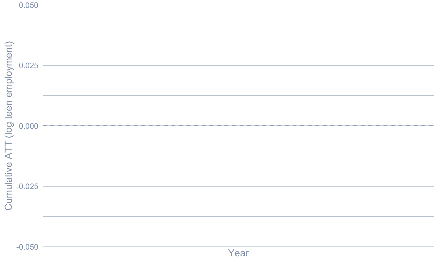
```{r}
#| label: fig-cumulative
#| fig-cap: "Cumulative ATT trajectory. The slope of the line at any year is the per-period effect; the line itself is the running total of treatment effect since the earliest treatment onset (year 2004). A roughly linear shape is consistent with chapter 9's event-study finding that effects accumulate over time."
#| fig-width: 7.5
#| fig-height: 4.5
ggplot(cumu_df, aes(x = Year, y = `Cumulative ATT`)) +
  geom_hline(yintercept = 0, color = "#94a3b8", linetype = "dashed") +
  geom_ribbon(aes(ymin = `CI lower`, ymax = `CI upper`),
              fill = "#22d3ee", alpha = 0.2) +
  geom_line(color = "#22d3ee", linewidth = 0.9) +
  geom_point(color = "#22d3ee", size = 2.5) +
  labs(x = "Year", y = "Cumulative ATT (log teen employment)")
```
## Inference: bootstrap variants compared
`gsynth` supports three inference modes: **parametric bootstrap**
(simulates residuals from the estimated error distribution),
**nonparametric bootstrap** (resamples units with replacement),
and **jackknife** (leave-one-unit-out). Each targets a slightly
different variance, and on short panels with few treated units the
three can diverge meaningfully.
```{r}
#| label: fit-inference-modes
#| message: false
#| warning: false
#| cache: true
out_np <- out   # already nonparametric from earlier fit

out_param <- gsynth(lemp ~ treat + lpop + lavg_pay,
                    data = mw_df,
                    index = c("id", "year"),
                    force = "two-way",
                    CV = FALSE, r = r_star,
                    se = TRUE,
                    inference = "parametric",
                    nboots = 500,
                    min.T0 = 3,
                    parallel = TRUE,
                    seed = 42)

out_jk <- gsynth(lemp ~ treat + lpop + lavg_pay,
                 data = mw_df,
                 index = c("id", "year"),
                 force = "two-way",
                 CV = FALSE, r = r_star,
                 se = TRUE,
                 inference = "jackknife",
                 min.T0 = 3,
                 parallel = TRUE,
                 seed = 42)
```
```{r}
#| label: tbl-inference-compare
#| tbl-cap: "Overall ATT under three uncertainty-quantification methods, holding $r = r^*$ constant. The point estimate is identical — inference choice only affects the standard error and CI. Nonparametric is the default in modern gsynth/fect practice; parametric assumes the residual distribution is right; jackknife is the most conservative."
extract_est <- function(o, label) {
  tibble(
    Method     = label,
    Estimate   = o$att.avg,
    `S.E.`     = o$est.avg[1, "S.E."],
    `CI lower` = o$est.avg[1, "CI.lower"],
    `CI upper` = o$est.avg[1, "CI.upper"],
    `p-value`  = o$est.avg[1, "p.value"]
  )
}

bind_rows(
  extract_est(out_np,    "Nonparametric bootstrap"),
  extract_est(out_param, "Parametric bootstrap"),
  extract_est(out_jk,    "Jackknife")
) |> gt_pretty(decimals = 4)
```
The three CIs usually agree in sign and significance when the
factor model fits well. When they disagree — typically with the
jackknife CI being noticeably wider than the nonparametric one —
that is a flag that the headline result hinges on one or two
influential treated units. Inspecting the leave-one-out trajectory
(or the factor-loading plot) usually identifies the culprit.
## Recap
::: {.callout-note appearance="simple"}
**The estimators reconciled.** On this Callaway-Sant'Anna
minimum-wage panel:
- gsynth with no factors ($r = 0$):
$\hat\tau \approx `r sprintf("%.3f", ic_tbl$ATT[ic_tbl$r == 0])`$
(close to chapter 9's TWFE coefficient of $-0.038$).
- gsynth with IC-selected factors ($r^* = `r r_star`$):
$\hat\tau \approx `r sprintf("%.3f", out$att.avg)`$.
- Chapter 9's Callaway-Sant'Anna overall ATT: $-0.057$.
- Chapter 9's doubly-robust conditional ATT: $-0.065$.
The factor-augmented gsynth estimate is in the same direction and
within sampling error of the chapter-9 staggered-DiD estimates.
Two estimators with very different identifying assumptions —
parallel trends in chapter 9, parallel factors here — pointing to
the same conclusion is the strongest possible evidence the design
generates.
**What gsynth buys.** Identification under a factor model that is
plausibly weaker than parallel trends when cohort-specific shocks
are at work. The counterfactual for each treated unit is a real
imputed series, not the residual of a regression — which makes
the substantive interpretation closer to SCM than to DiD.
**What it costs.** It needs enough pre-treatment depth to identify
factors. Our cohort 2004 only just clears the threshold; cohort
2006 is comfortable. The standard errors widen sharply with more
factors when the panel is short, as the IC table shows. And when
a treated unit's factor-loading vector falls outside the convex
hull of control loadings, the imputation extrapolates rather than
interpolates — a real-world failure mode that the `fect` package's
simplex-loading projection addresses (see Further reading).
:::
## Common pitfall
Treating a gsynth fit as automatically valid because it "uses
factors". Three diagnostics together are what justify the
headline:
1. **Pre-treatment fit in the gap plot.** If the pre-period gap
wanders away from zero, the factor model is missing something —
not absorbing the relevant comovement.
2. **IC across $r$.** If multiple $r$ values give nearly identical
IC but very different ATTs, the headline is fragile to the
factor count and you should report sensitivity.
3. **Convex-hull check in the loadings plot.** Treated units far
outside the cloud of control loadings are being extrapolated
to, not interpolated to, and their imputed counterfactuals are
correspondingly less trustworthy.
If any of those three look bad, the headline ATT should be
presented with conspicuous caveats — or paired with a method whose
failure modes differ, such as the chapter-9 doubly-robust DiD.
## Further reading
@xu2017generalized is the canonical reference and remains the
clearest exposition of the method. The companion *fect* tutorial
at <https://yiqingxu.org/packages/fect/06-gsynth.html> shows the
same estimator with a richer API: a simplex projection that
bounds treated loadings to the convex hull of control loadings
(addressing the extrapolation problem above), equivalence tests
for pre-treatment fit, and matrix-completion variants
[@athey2021matrix]. Chapter 10 of this book takes that broader
view; this chapter is the focused walkthrough of the gsynth
estimator alone.
## Exercises
1. Re-run the IC grid with $r = 3$ and $r = 4$. Does the IC keep
falling, level off, or rise? At what point does the standard
error become uninformative, and what does that tell you about
the effective rank of the never-treated panel?
2. Drop the `lpop + lavg_pay` covariates from the formula. Does
the ATT move? What does that say about whether the factors are
already absorbing variation in population and pay trajectories?
3. Compare gsynth's overall ATT to the doubly-robust
Callaway-Sant'Anna estimate from chapter 9 ($-0.065$). Which
one would you report as the headline, and what design feature
of the data drives your choice?