3 Regression Discontinuity in Time

3.1 The RDD-on-time idea

Regression Discontinuity in Time treats the calendar year itself as the running variable and the policy date as a sharp threshold. We fit a piecewise linear regression to California’s full 1970–2000 series that allows two breaks at 1989:

A level jump at the threshold — the immediate “policy shock”.
A slope change after the threshold — how the trajectory bends afterwards.

The level jump is the headline RDD effect. The slope change is the medium-run trajectory.

A naming heads-up. The workshop labels this specification “RDD”. It is RDD with time as the running variable, not the classical sharp RDD you would use for a means-tested benefit at an income cutoff. With time as the running variable, the math reduces to segmented regression.

3.2 The equation

Re-centre time at the threshold by defining $\tilde t = t - t^* - 1$ (so $\tilde t = 0$ for the first post-period year). Then fit the segmented regression

\[Y_{1t} = \beta_0 + \beta_1\, \tilde t + \beta_2\, \mathbf{1}[\tilde t \ge 0] + \beta_3\, \tilde t \cdot \mathbf{1}[\tilde t \ge 0] + \varepsilon_t.\]

Each coefficient has a precise causal reading.

$\beta_0$ is the pre-period intercept at $\tilde t = 0$ (California’s fitted level just before the threshold).
$\beta_1$ is the pre-period slope.
$\beta_2$ is the level break at the threshold — the immediate jump in cigarette sales at $\tilde t = 0$. This is the headline RDD effect.
$\beta_3$ is the change in slope after the threshold (the post-period slope is $\beta_1 + \beta_3$).

The piecewise counterfactual continues the pre-period line ($\beta_0 + \beta_1\, \tilde t$) into the post-period, so the total deviation of observed from counterfactual at time $\tilde t > 0$ is $\beta_2 + \beta_3\, \tilde t$. The policy shifts the series down by $\beta_2$ packs immediately, then the gap widens (or narrows) at rate $\beta_3$ per year.

3.3 Setup and data

Packages. tidyverse covers data wrangling and plotting. sandwich and lmtest provide the HAC-robust standard errors used in the regression below — short autocorrelated time series need them, because the textbook OLS SEs would be wildly overconfident. fpp3 is loaded only for the tsibble class (we don’t actually forecast in this chapter, but reusing the chapter-2 dataset shape keeps the wrangling brief). The R/table_helpers.R helper provides ms_pretty(), the modelsummary wrapper that styles the regression table further down.

Code

library(tidyverse)
library(sandwich)
library(lmtest)
library(fpp3)   # for tsibble class
source("R/table_helpers.R")

set.seed(42)

knitr::opts_chunk$set(dev.args = list(bg = "transparent"))

theme_set(
  theme_minimal(base_size = 12) +
    theme(
      plot.background  = element_rect(fill = "transparent", color = NA),
      panel.background = element_rect(fill = "transparent", color = NA),
      panel.grid.major = element_line(color = "#94a3b8", linewidth = 0.25),
      panel.grid.minor = element_line(color = "#94a3b8", linewidth = 0.15),
      text             = element_text(color = "#94a3b8"),
      axis.text        = element_text(color = "#94a3b8")
    )
)

Dataset. As in chapter 2 we collapse the 39-state panel to a California-only tsibble covering 1970–2000. The crucial new piece is the centred index year0 = year − 1989: it makes the policy threshold land at zero. In RDD-on-time language, year0 is the running variable, the threshold is year0 = 0, and the level break at the threshold is the headline RDD effect.

Code

prop99 <- read_rds("data/proposition99.rds") |> as_tibble()

prop99_ts <- prop99 |>
  filter(state == "California") |>
  select(year, cigsale) |>
  mutate(prepost = factor(year > 1988, labels = c("Pre", "Post"))) |>
  as_tsibble(index = year) |>
  mutate(year0 = year - 1989)

The resulting prop99_ts has 31 rows × 4 columns: year, cigsale, prepost (the Pre/Post factor), and year0 (the centred running variable). All four columns appear in the regression specification below.

3.4 Fit and HAC inference

The fit. The piecewise regression cigsale ~ year0 + prepost + year0:prepost is the direct translation of the four-coefficient equation from the previous section: an intercept, a pre-period slope on year0, a level break at the threshold (prepostPost), and a slope change after the threshold (the year0:prepostPost interaction). The fit uses the full 1970–2000 series — not just a narrow bandwidth around the threshold — because with annual data we only have 19 pre-period and 12 post-period years to begin with. We pair the OLS coefficients with HAC-robust standard errors via sandwich::vcovHAC, which corrects for the autocorrelation and heteroskedasticity that annual outcome series typically exhibit; classical OLS SEs here would understate uncertainty by roughly half.

Code

# Piecewise OLS: pre-period slope, level break at threshold, slope change
# after threshold. year0 = year - 1989 (already constructed above).
fit_rdd <- lm(cigsale ~ year0 + prepost + year0:prepost,
              data = as_tibble(prop99_ts))

# HAC-robust standard errors for the four coefficients.
ms_pretty(list("Piecewise OLS, HAC SEs" = fit_rdd),
          vcov     = sandwich::vcovHAC,
          coef_map = c("(Intercept)"         = "Pre-period intercept",
                       "year0"               = "Pre-period slope",
                       "prepostPost"         = "Level break at 1989",
                       "year0:prepostPost"   = "Slope change post-1989"),
          notes    = "Standard errors HAC-robust via sandwich::vcovHAC.")

Table 3.1: RD-in-time fit (HAC-robust SEs).

	Piecewise OLS, HAC SEs
Pre-period intercept	98.416***
	(4.968)
Pre-period slope	-1.779***
	(0.459)
Level break at 1989	-20.058**
	(5.585)
Slope change post-1989	-1.495***
	(0.401)
Num.Obs.	31
R2	0.973
Std.Errors	Custom
+ p < 0.1, * p < 0.05, p < 0.01, * p < 0.001
Standard errors HAC-robust via sandwich::vcovHAC.

Reading the output. Three coefficients matter.

Pre-period slope year0 ≈ $-1.78$ packs/year. Matches the ITS-growth fit from chapter 2; sanity check passed.
Level break prepostPost ≈ $-20.06$ packs (HAC SE ≈ 5.59, $p \approx 0.001$). California’s sales drop by about 20 packs immediately at the 1989 threshold.
Slope change year0:prepostPost ≈ $-1.49$ packs/year (HAC SE ≈ 0.40, $p < 0.001$). The post-period decline accelerates by an extra 1.5 packs/year on top of the pre-period 1.8 packs/year.

Combining the level break and the slope change, by 2000 (11 years after the threshold) the cumulative deviation from the extrapolated pre-trend is roughly $-20 - 11 \times 1.49 \approx -36$ packs. The piecewise fit is excellent ($R^2 \approx 0.97$).

3.5 Visual diagnostic

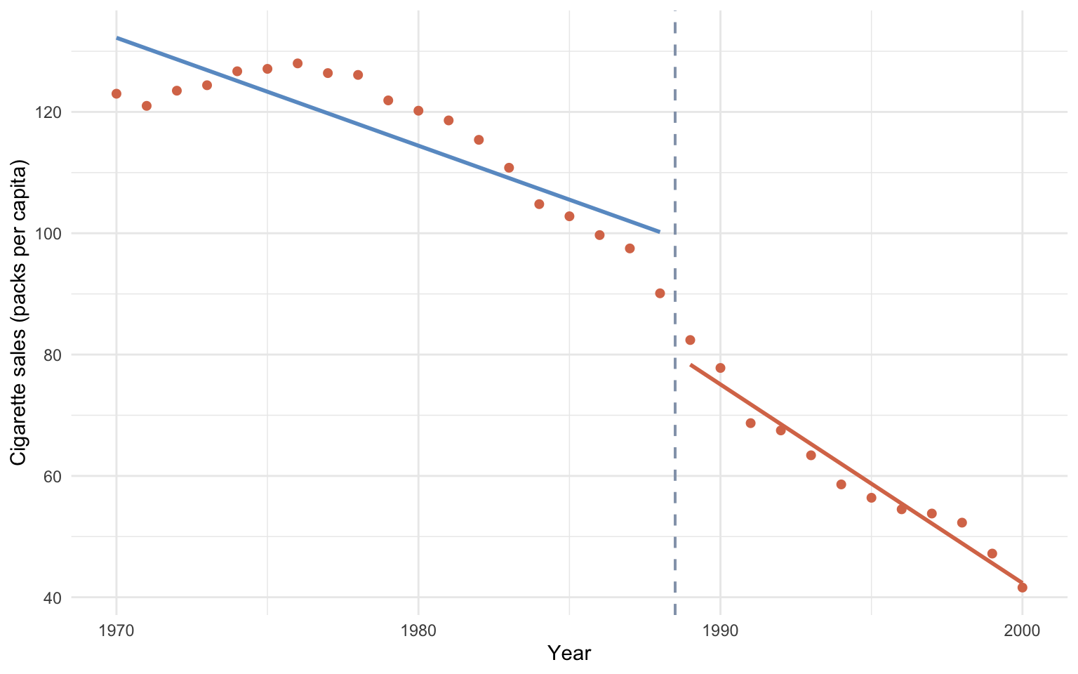
What to look for. The plot below overlays California’s annual cigarette-sales points with two separately fit geom_smooth(method = "lm") lines — blue for the pre-1989 segment, orange for the post-1989 segment — meeting at the dashed vertical at year0 = 0. Three features are worth checking by eye: (1) the vertical gap between the two lines at the threshold (that gap is the prepostPost coefficient — the level break); (2) the change in slope across the threshold (that’s the year0:prepostPost interaction — the trajectory bend); and (3) whether the points hug both lines tightly (poor fit anywhere would warn that the piecewise-linear specification is misspecified for the underlying process).

Code

plot_df <- as_tibble(prop99_ts)

ggplot(plot_df, aes(x = year, y = cigsale)) +
  geom_point(color = "#d97757", size = 1.8) +
  geom_smooth(data = filter(plot_df, prepost == "Pre"),
              method = "lm", se = FALSE, color = "#6a9bcc", linewidth = 1) +
  geom_smooth(data = filter(plot_df, prepost == "Post"),
              method = "lm", se = FALSE, color = "#d97757", linewidth = 1) +
  geom_vline(xintercept = 1988.5, color = "#94a3b8",
             linetype = "dashed", linewidth = 0.7) +
  labs(x = "Year", y = "Cigarette sales (packs per capita)") +
  theme_minimal()

Figure 3.1: RDD on time: piecewise pre/post linear fit with level and slope breaks at 1989.

The blue pre-1988 line and the orange post-1989 line both fit California’s points almost perfectly, with a clear discontinuity at the threshold.

3.6 Caveats

RDD on time inherits the same pre-trend mis-specification risk as ITS. If California’s underlying trajectory was already changing curvature in the late 1980s for non-policy reasons — say, the 1988 Surgeon General’s report on nicotine addiction — the level break attributed to Proposition 99 will absorb that change too.

Common pitfall. Mistaking a coincident shock at the threshold for the policy effect. With time as the running variable, any event that happens to land in the same year as the policy — a related federal regulation, a recession, a media campaign — is absorbed into the level break.

Recap. Regression Discontinuity on time reports a $-20.1$ pack level break with a tight standard error. It is the first of three methods in the book to land in the credible $-13$ to $-20$ “consensus” range, alongside Synthetic Control (chapter 5) and the Bayesian structural TS model (chapter 6).

3.7 Further reading

For classical sharp RDD on a continuous running variable (test scores, income, age), use rdrobust by Calonico, Cattaneo & Titiunik instead of the segmented-regression approach above.

--- title: "Regression Discontinuity in Time" --- ## The RDD-on-time idea Regression Discontinuity in Time treats the **calendar year** itself as the running variable and the policy date as a sharp threshold. We fit a piecewise linear regression to California's full 1970–2000 series that allows two breaks at 1989: - A **level jump** at the threshold — the immediate "policy shock". - A **slope change** after the threshold — how the trajectory bends afterwards. The level jump is the headline RDD effect. The slope change is the medium-run trajectory. **A naming heads-up.** The workshop labels this specification "RDD". It is RDD with time as the running variable, not the classical sharp RDD you would use for a means-tested benefit at an income cutoff. With time as the running variable, the math reduces to *segmented regression*. ## The equation Re-centre time at the threshold by defining $\tilde t = t - t^* - 1$ (so $\tilde t = 0$ for the first post-period year). Then fit the segmented regression $$Y_{1t} = \beta_0 + \beta_1\, \tilde t + \beta_2\, \mathbf{1}[\tilde t \ge 0] + \beta_3\, \tilde t \cdot \mathbf{1}[\tilde t \ge 0] + \varepsilon_t.$$ Each coefficient has a precise causal reading. - $\beta_0$ is the pre-period intercept at $\tilde t = 0$ (California's fitted level just before the threshold). - $\beta_1$ is the *pre-period* slope. - $\beta_2$ is the **level break** at the threshold — the immediate jump in cigarette sales at $\tilde t = 0$. This is the headline RDD effect. - $\beta_3$ is the **change in slope** after the threshold (the post-period slope is $\beta_1 + \beta_3$). The piecewise counterfactual continues the pre-period line ($\beta_0 + \beta_1\, \tilde t$) into the post-period, so the total deviation of observed from counterfactual at time $\tilde t > 0$ is $\beta_2 + \beta_3\, \tilde t$. The policy shifts the series *down* by $\beta_2$ packs immediately, then the gap widens (or narrows) at rate $\beta_3$ per year. ## Setup and data **Packages.** `tidyverse` covers data wrangling and plotting. `sandwich` and `lmtest` provide the HAC-robust standard errors used in the regression below — short autocorrelated time series need them, because the textbook OLS SEs would be wildly overconfident. `fpp3` is loaded only for the `tsibble` class (we don't actually forecast in this chapter, but reusing the chapter-2 dataset shape keeps the wrangling brief). The `R/table_helpers.R` helper provides `ms_pretty()`, the `modelsummary` wrapper that styles the regression table further down. ```{r} #| label: setup #| message: false #| warning: false library(tidyverse) library(sandwich) library(lmtest) library(fpp3) # for tsibble class source("R/table_helpers.R") set.seed(42) knitr::opts_chunk$set(dev.args = list(bg = "transparent")) theme_set( theme_minimal(base_size = 12) + theme( plot.background = element_rect(fill = "transparent", color = NA), panel.background = element_rect(fill = "transparent", color = NA), panel.grid.major = element_line(color = "#94a3b8", linewidth = 0.25), panel.grid.minor = element_line(color = "#94a3b8", linewidth = 0.15), text = element_text(color = "#94a3b8"), axis.text = element_text(color = "#94a3b8") ) ) ``` **Dataset.** As in chapter 2 we collapse the 39-state panel to a California-only `tsibble` covering 1970–2000. The crucial new piece is the centred index `year0 = year − 1989`: it makes the policy threshold land at zero. In RDD-on-time language, `year0` is the **running variable**, the threshold is `year0 = 0`, and the level break at the threshold is the headline RDD effect. ```{r} #| label: data-load prop99 <- read_rds("data/proposition99.rds") |> as_tibble() prop99_ts <- prop99 |> filter(state == "California") |> select(year, cigsale) |> mutate(prepost = factor(year > 1988, labels = c("Pre", "Post"))) |> as_tsibble(index = year) |> mutate(year0 = year - 1989) ``` The resulting `prop99_ts` has 31 rows × 4 columns: `year`, `cigsale`, `prepost` (the Pre/Post factor), and `year0` (the centred running variable). All four columns appear in the regression specification below. ## Fit and HAC inference **The fit.** The piecewise regression `cigsale ~ year0 + prepost + year0:prepost` is the direct translation of the four-coefficient equation from the previous section: an intercept, a pre-period slope on `year0`, a level break at the threshold (`prepostPost`), and a slope change after the threshold (the `year0:prepostPost` interaction). The fit uses the full 1970–2000 series — *not* just a narrow bandwidth around the threshold — because with annual data we only have 19 pre-period and 12 post-period years to begin with. We pair the OLS coefficients with HAC-robust standard errors via `sandwich::vcovHAC`, which corrects for the autocorrelation and heteroskedasticity that annual outcome series typically exhibit; classical OLS SEs here would understate uncertainty by roughly half. ```{r} #| label: tbl-fit-rdd #| tbl-cap: "RD-in-time fit (HAC-robust SEs)." # Piecewise OLS: pre-period slope, level break at threshold, slope change # after threshold. year0 = year - 1989 (already constructed above). fit_rdd <- lm(cigsale ~ year0 + prepost + year0:prepost, data = as_tibble(prop99_ts)) # HAC-robust standard errors for the four coefficients. ms_pretty(list("Piecewise OLS, HAC SEs" = fit_rdd), vcov = sandwich::vcovHAC, coef_map = c("(Intercept)" = "Pre-period intercept", "year0" = "Pre-period slope", "prepostPost" = "Level break at 1989", "year0:prepostPost" = "Slope change post-1989"), notes = "Standard errors HAC-robust via sandwich::vcovHAC.") ``` **Reading the output.** Three coefficients matter. 1. **Pre-period slope `year0` ≈ $-1.78$ packs/year.** Matches the ITS-growth fit from chapter 2; sanity check passed. 2. **Level break `prepostPost` ≈ $-20.06$ packs** (HAC SE ≈ 5.59, $p \approx 0.001$). California's sales drop by about 20 packs *immediately* at the 1989 threshold. 3. **Slope change `year0:prepostPost` ≈ $-1.49$ packs/year** (HAC SE ≈ 0.40, $p < 0.001$). The post-period decline accelerates by an extra 1.5 packs/year *on top of* the pre-period 1.8 packs/year. Combining the level break and the slope change, by 2000 (11 years after the threshold) the cumulative deviation from the extrapolated pre-trend is roughly $-20 - 11 \times 1.49 \approx -36$ packs. The piecewise fit is excellent ($R^2 \approx 0.97$). ## Visual diagnostic **What to look for.** The plot below overlays California's annual cigarette-sales points with two separately fit `geom_smooth(method = "lm")` lines — blue for the pre-1989 segment, orange for the post-1989 segment — meeting at the dashed vertical at `year0 = 0`. Three features are worth checking by eye: (1) the *vertical gap* between the two lines at the threshold (that gap is the `prepostPost` coefficient — the level break); (2) the *change in slope* across the threshold (that's the `year0:prepostPost` interaction — the trajectory bend); and (3) whether the points hug both lines tightly (poor fit anywhere would warn that the piecewise-linear specification is misspecified for the underlying process). ```{r} #| label: fig-rdd-segmented #| fig-cap: "RDD on time: piecewise pre/post linear fit with level and slope breaks at 1989." #| fig-width: 8 #| fig-height: 5 #| message: false plot_df <- as_tibble(prop99_ts) ggplot(plot_df, aes(x = year, y = cigsale)) + geom_point(color = "#d97757", size = 1.8) + geom_smooth(data = filter(plot_df, prepost == "Pre"), method = "lm", se = FALSE, color = "#6a9bcc", linewidth = 1) + geom_smooth(data = filter(plot_df, prepost == "Post"), method = "lm", se = FALSE, color = "#d97757", linewidth = 1) + geom_vline(xintercept = 1988.5, color = "#94a3b8", linetype = "dashed", linewidth = 0.7) + labs(x = "Year", y = "Cigarette sales (packs per capita)") + theme_minimal() ``` The blue pre-1988 line and the orange post-1989 line both fit California's points almost perfectly, with a clear discontinuity at the threshold. ## Caveats RDD on time inherits the same pre-trend mis-specification risk as ITS. If California's *underlying* trajectory was already changing curvature in the late 1980s for non-policy reasons — say, the 1988 Surgeon General's report on nicotine addiction — the level break attributed to Proposition 99 will absorb that change too. **Common pitfall.** Mistaking a coincident shock at the threshold for the policy effect. With time as the running variable, *any* event that happens to land in the same year as the policy — a related federal regulation, a recession, a media campaign — is absorbed into the level break. **Recap.** Regression Discontinuity on time reports a $-20.1$ pack level break with a tight standard error. It is the first of three methods in the book to land in the credible $-13$ to $-20$ "consensus" range, alongside Synthetic Control (chapter 5) and the Bayesian structural TS model (chapter 6). ## Further reading - For classical sharp RDD on a continuous running variable (test scores, income, age), use `rdrobust` by Calonico, Cattaneo & Titiunik instead of the segmented-regression approach above.