flowchart TB
    subgraph "BSTS counterfactual ŷ₁ₜ"
        TREND["μₜ — local-level trend<br/>(absorbs dynamics no control can explain)"]
        REG["β·xₜ — regression on donor cigsale + covariates<br/>(borrows from donor pool)"]
        ERR["εₜ — random error"]
    end
    TREND --> Y["ŷ₁ₜ"]
    REG --> Y
    ERR --> Y
    Y --> CMP["Observed y₁ₜ − ŷ₁ₜ<br/>= policy effect (with credible band)"]

    style TREND fill:#6a9bcc,stroke:#cbd5e0,color:#fff
    style REG fill:#00d4c8,stroke:#cbd5e0,color:#141413
    style ERR fill:#7a8395,stroke:#cbd5e0,color:#fff
    style Y fill:#7A209F,stroke:#cbd5e0,color:#fff
    style CMP fill:#d97757,stroke:#cbd5e0,color:#fff
6 Structural Bayesian Time Series
6.1 The BSTS / CausalImpact idea
Fit a Bayesian structural time-series (BSTS) model on the pre-period. Use other states’ cigarette sales (and optionally covariates) as predictors. Project the fitted model forward as the counterfactual. The posterior over (observed − projected) gives a credible interval for the policy effect.
This is the only method in the book that delivers a credible interval — a direct probability statement about the parameter — rather than a frequentist confidence band or a Fisher exact \(p\)-value.
6.2 The model in two pieces
The BSTS counterfactual is
\[y_{1t} = \mu_t + \beta^\top x_t + \varepsilon_t, \quad t \le t^*\]
where \(\mu_t\) is a local-level trend, \(x_t\) are the control-series regressors (other states’ cigsale, plus optional covariates), and \(t^*\) is the intervention date. California’s outcome is a slowly-evolving trend plus a linear combination of donor-state series plus a random error.
The trend \(\mu_t\) absorbs the dynamics that no control series can explain; the regression term \(\beta^\top x_t\) borrows information from the donor pool. After the model is fit on \(t \le t^*\), it is projected forward and the posterior over \(y_{1t} - \hat{y}_{1t}\) gives the credible interval for the policy effect.
6.3 Setup and data
Packages. tidyverse covers wrangling and plotting. CausalImpact is Google’s wrapper around the bsts (Bayesian Structural Time Series) package: it takes a wide matrix with the treated outcome in column 1 and donor series in the remaining columns, fits a Bayesian state-space model on the pre-period, projects forward as the counterfactual, and returns posterior means + 95% credible intervals on the pointwise and cumulative effects. mice provides multiple imputation by chained equations — we use its random-forest mode to fill the missing covariate values before pivoting to wide form. The R/table_helpers.R helper provides gt_pretty() for the summary table.
Code
library(tidyverse)
library(CausalImpact)
library(mice)
source("R/table_helpers.R")

set.seed(42)

knitr::opts_chunk$set(dev.args = list(bg = "transparent"))

theme_set(
  theme_minimal(base_size = 12) +
    theme(
      plot.background  = element_rect(fill = "transparent", color = NA),
      panel.background = element_rect(fill = "transparent", color = NA),
      panel.grid.major = element_line(color = "#94a3b8", linewidth = 0.25),
      panel.grid.minor = element_line(color = "#94a3b8", linewidth = 0.15),
      text             = element_text(color = "#94a3b8"),
      axis.text        = element_text(color = "#94a3b8")
    )
)
Dataset. Like Synthetic Control, this method uses the full 39-state × 31-year panel: every state other than California is potentially a regressor in the Bayesian counterfactual model, and the four covariates (lnincome, retprice, age15to24, beer) are candidate predictors too. We do not pre-filter or restrict the window. The dataset is loaded as-is and then reshaped from long to wide in the next section, which is the form CausalImpact requires.
Code
prop99 <- read_rds("data/proposition99.rds") |> as_tibble()The loaded prop99 is the same 1,209-row × 7-column tibble used in chapter 5 (39 states × 31 years × the cigsale outcome and four covariates). The next section deals with the missing covariate values and the long-to-wide reshape that CausalImpact requires.
6.4 Imputation and wide pivot
CausalImpact wants a wide dataset with the treated outcome in column 1 and every control series in the remaining columns. The covariate columns have missing values (lnincome is missing 16% of rows, age15to24 32%, beer 55%), so we fill them with single random-forest imputation from mice.
Code
# Fill in missing covariate values with one round of random-forest
# multiple imputation (m = 1, method = "rf"). printFlag suppresses
# console chatter.
prop99_imputed <- prop99 |>
  mice(m = 1, method = "rf", printFlag = FALSE) |>
  complete() |>
  as_tibble()

# Pivot the long panel to wide format: one column per (variable, state)
# pair. CausalImpact requires the treated outcome in column 1, hence
# relocate(cigsale_California) and drop the year index.
prop99_wide <- prop99_imputed |>
  pivot_wider(names_from  = state,
              values_from = c(cigsale, lnincome, beer, age15to24, retprice)) |>
  relocate(cigsale_California) |>
  select(-year)

dim(prop99_wide)
[1] 31 195The reported dim() confirms the reshape: prop99_wide is 31 rows × 195 columns — one row per year 1970–2000, and 39 states × 5 variables in the columns (cigsale_*, lnincome_*, beer_*, age15to24_*, retprice_* for each of the 39 states), with year dropped and cigsale_California relocated to column 1 because that’s what CausalImpact() expects as the treated outcome.
6.5 Fit the Bayesian structural TS model
The fit. The chunk below calls CausalImpact(prop99_wide, pre.period, post.period) with the pre and post windows expressed as integer row indices (not years): row 1 is 1970, row 19 is 1988 (the last pre-period year), row 20 is 1989, row 31 is 2000. The seed is reset just before the call because bsts uses an MCMC sampler under the hood; a fixed seed makes the posterior draws reproducible from one render to the next. The returned impact_full$summary is a two-row data frame — one row for the average effect over 1989–2000 and one row for the cumulative effect — with posterior means and 95% credible bounds for each. The helper code below the CausalImpact() call just formats those columns into the table.
Code
# CausalImpact takes integer row indices, not years.
# Row 1 = 1970, row 19 = 1988 (last pre-period year).
# Row 20 = 1989, row 31 = 2000 (last observed year).
pre_idx  <- c(1, 19)
post_idx <- c(20, 31)

# Reset the seed so the BSTS MCMC draws are reproducible.
set.seed(42)

impact_full <- CausalImpact(prop99_wide,
                            pre.period  = pre_idx,
                            post.period = post_idx)

ci_summary <- impact_full$summary |>
  tibble::rownames_to_column("Horizon") |>
  dplyr::transmute(
    Horizon,
    Actual            = sprintf("%.1f", Actual),
    Prediction        = sprintf("%.1f [%.1f, %.1f]",
                                Pred, Pred.lower, Pred.upper),
    `Absolute effect` = sprintf("%.1f [%.1f, %.1f]",
                                AbsEffect, AbsEffect.lower, AbsEffect.upper),
    `Relative effect` = sprintf("%.1f%% [%.1f%%, %.1f%%]",
                                RelEffect * 100, RelEffect.lower * 100,
                                RelEffect.upper * 100),
    `Posterior p`     = sprintf("%.3f", p)
  )

gt_pretty(ci_summary)| Horizon | Actual | Prediction | Absolute effect | Relative effect | Posterior p |
|---|---|---|---|---|---|
| Average | 60.4 | 73.2 [54.7, 92.3] | -12.8 [-31.9, 5.7] | -15.9% [-34.6%, 10.4%] | 0.082 |
| Cumulative | 724.2 | 878.1 [656.1, 1107.6] | -153.9 [-383.4, 68.1] | -15.9% [-34.6%, 10.4%] | 0.082 |
Reading the output.
- Average ATT: approximately \(-13\) packs/capita (posterior SD ≈ 11), 95% credible interval roughly \([-32, +5.7]\).
- Cumulative effect: about \(-154\) packs over 12 years, or roughly 16% of what would have been expected absent the policy.
- Posterior probability of any causal effect: ≈ 92%.
If we drop the covariates and use only other states’ cigarette sales as controls, the point estimate strengthens to around \(-21\) packs and the posterior probability rises to ≈ 97%. The covariates absorb some of the variation the simpler model was attributing to Proposition 99 — which can be read as either “added robustness” or “watered-down signal” depending on how much you trust the imputed beer-and-income covariates.
6.6 The two-panel diagnostic
What to look for. Calling plot() on a CausalImpact object returns its default two-panel figure: the top panel shows observed California (solid line) against the Bayesian counterfactual (dashed) with its 95% credible band; the bottom panel shows the cumulative gap — the running sum of observed − counterfactual from the intervention date onwards, with its own credible band. Read the top panel for whether and when the policy effect opens up, and the bottom panel for whether the cumulative effect’s credible band excludes zero by the end of the series.
Code
plot(impact_full)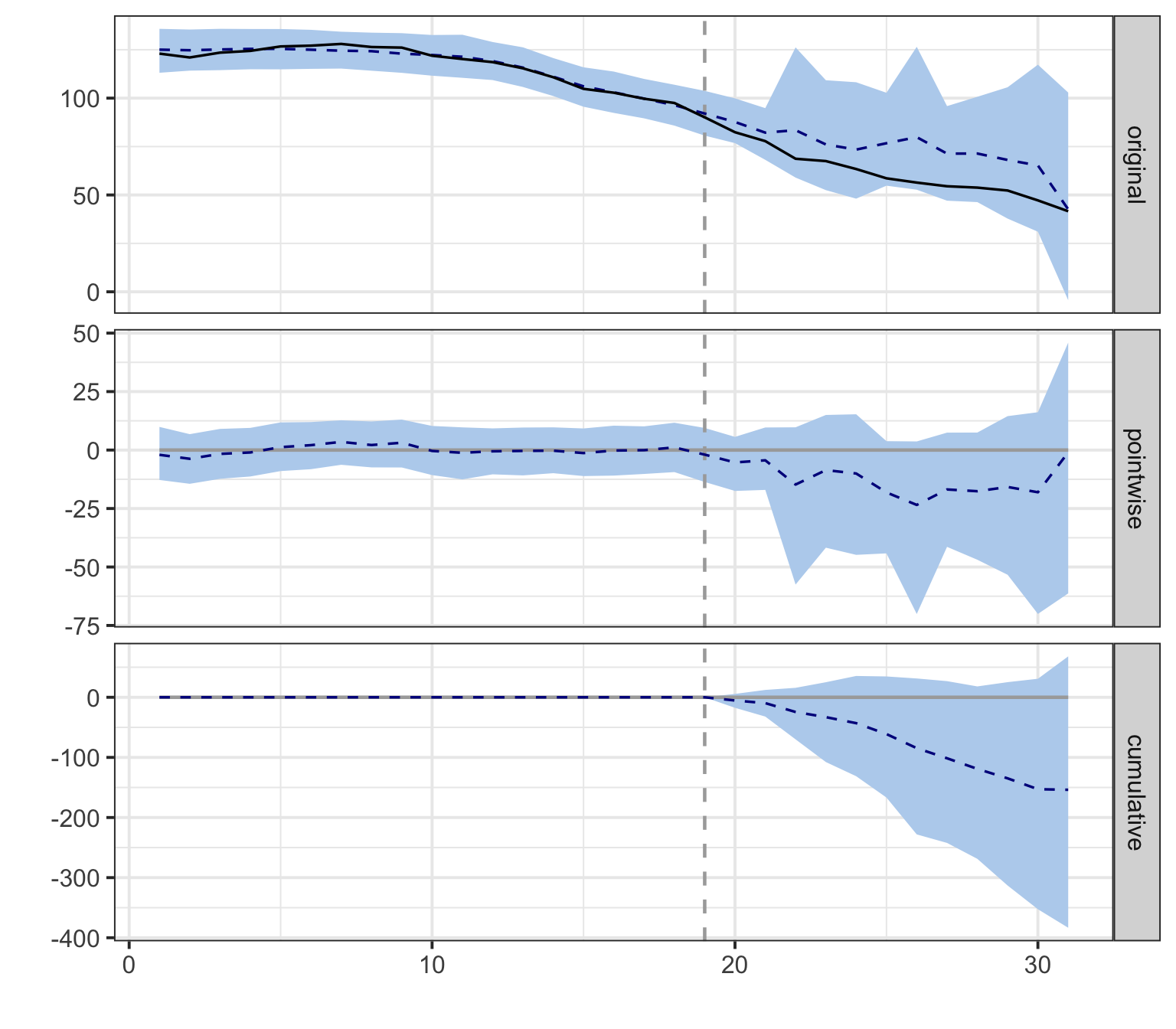
The top panel shows the pointwise picture: observed California opens a steady gap below the Bayesian counterfactual starting in 1989, with a 95% credible band that widens as we forecast further from the training window. The bottom panel cumulates that gap over time. By 2000 the cumulative effect is roughly \(-150\) packs/capita with a credible interval that includes zero only at the very upper edge.
6.7 Common pitfall
Imputing missing covariates without thinking about the imputation model. The random-forest fill we use here is a single-imputation shortcut for tutorial speed. With multiple imputation (\(m > 1\)) or a different model, the estimate can move by 1–3 packs. Two concrete failure modes are worth spelling out, because they affect the credibility of the headline number rather than just its width.
Example 1 — Imputing donor covariates with a model that “sees” California. Our mice(prop99, ...) call passes the entire panel — California rows included — into the imputation model. For this dataset, with only four covariates and most missingness clustered in beer (≈55%) and age15to24 (≈32%) on donor states, the consequence is usually mild. But if you were to feed the full panel with the post-period California outcome attached into an imputer that also uses cigsale as a predictor, the imputer could learn from California’s post-1989 trajectory and propagate that information back into donor states’ missing covariate cells. CausalImpact would then build a counterfactual that mechanically tracks California’s post-period — biasing the estimated effect toward zero by construction. The safe pattern is to impute donor covariates before the treated outcome is in scope, or to drop the treated unit from the imputer entirely and impute donors only.
Example 2 — Single (m = 1) vs multiple (m = 5) imputation. Single imputation treats the imputed values as if they were observed, then propagates that pretend-observed dataset through CausalImpact. The posterior credible band you get back is the model’s uncertainty given the imputed cells — it knows nothing about the uncertainty introduced by the imputation itself. With proper multiple imputation (mice(..., m = 5) and Rubin’s-rules pooling across the five resulting fits), the credible band widens by roughly 1–3 packs on this dataset because the across-imputation variance is added to the within-imputation variance. The point estimate barely moves; the interval does. For a tutorial we keep m = 1 for speed and clarity, but a published number should use m ≥ 5 and report a pooled estimate.
6.8 Recap
CausalImpact lands at \(-13\) to \(-21\) packs depending on whether covariates are included, with a 92–97% posterior probability of a non-zero effect. It is the only method in the book that delivers a credible interval (a direct probability statement about the parameter), not a frequentist confidence band.
| Question | Answer |
|---|---|
| What does CausalImpact estimate? | The ATT on California, 1989–2000 |
| What is the point estimate? | Average ≈ \(-13\) packs/capita; cumulative ≈ \(-154\) packs over 12 years |
| What is the uncertainty quantification? | 95% Bayesian credible interval ≈ \([-32, +5.7]\) packs; posterior probability of any effect ≈ 92% |
| How is the counterfactual built? | Local-level trend + Bayesian regression on donor-state cigarette sales (+ imputed covariates) |
| What is the design-time pitfall? | Single-imputation shortcuts on covariates with high missingness; never impute donors using the treated unit |