10 Matrix Completion and Interactive Fixed Effects

10.1 When parallel trends isn’t enough

Chapter 9 squeezed every drop of usable signal out of the Callaway-Sant’Anna minimum-wage panel under one identifying assumption: parallel trends. Conditional or unconditional, with or without never-treated counties, with or without anticipation slack, with Rambachan-Roth bounds on top — the assumption is always that, absent treatment, the trajectory of the treated counties would have moved in parallel with the untreated.

What if it would not have? Counties select into raising the minimum wage non-randomly. They are not a random subset of the country in the time-varying dimension either: industry mix, demographics, and local growth trends all shape both treatment timing and outcome paths. Two counties can share an industry-mix-driven trajectory that TWFE never absorbs — and so cannot net out.

This chapter relaxes parallel trends in a specific way. We model the counterfactual outcome as a factor structure:

\[Y_{it}(0) \;=\; \alpha_i + \xi_t + \lambda_i' f_t + \varepsilon_{it}.\]

Each unit $i$ has a loading vector $\lambda_i$; each period a factor vector $f_t$. Their interaction $\lambda_i' f_t$ encodes time-varying unobserved heterogeneity that no county or year fixed effect can absorb. Two views of the same object give two estimators (Liu et al., 2024):

Interactive Fixed Effects (IFEct) (Bai, 2009; Xu, 2017) treats $(\alpha, \xi, \Lambda, F)$ as parameters to be estimated on control observations, then imputes $Y_{it}(0)$ on treated cells.
Matrix Completion (MC) (Athey et al., 2021) reframes the same problem as filling missing entries of the implicit $Y(0)$ matrix: mask the treated cells, then complete via nuclear-norm-regularised SVD.

Yiqing Xu’s fect package implements both with a common API and a common counterfactual-plot diagnostic. By chapter’s end we line up its IFE and MC estimates next to the Callaway-Sant’Anna ATT from chapter 9 on the same panel — three estimands, three identifying assumptions, one substantive question.

10.2 Setup and data

Code

library(tidyverse)
library(fect)
library(panelView)
library(did)
library(patchwork)
source("R/table_helpers.R")

set.seed(42)

knitr::opts_chunk$set(dev.args = list(bg = "transparent"))

theme_set(
  theme_minimal(base_size = 12) +
    theme(
      plot.background  = element_rect(fill = "transparent", color = NA),
      panel.background = element_rect(fill = "transparent", color = NA),
      panel.grid.major = element_line(color = "#94a3b8", linewidth = 0.25),
      panel.grid.minor = element_line(color = "#94a3b8", linewidth = 0.15),
      text             = element_text(color = "#94a3b8"),
      axis.text        = element_text(color = "#94a3b8"),
      strip.text       = element_text(color = "#94a3b8"),
      legend.text      = element_text(color = "#94a3b8")
    )
)

We work from the same cs_minwage.rds panel as chapter 9, but with one small adjustment: factor-based estimators need at least as many pre-treatment periods per cohort as the number of factors they try to fit. Chapter 9’s 2003-2007 window leaves the 2004 cohort with only one pre-period, which would force min.T0 = 1 and cap the rank at zero — collapsing IFEct back to TWFE. So we widen the pre-treatment window by two years to 2001-2007; everything else (cohort filter, region drop, treatment indicator) is identical.

Code

mw_raw <- readRDS("data/cs_minwage.rds") |> as_tibble()

mw <- mw_raw |>
  filter(G %in% c(0, 2004, 2006, 2007), region != "1") |>
  filter(G != 2007, year >= 2001) |>
  mutate(D = as.integer(year >= G & G != 0))

dim(mw)

[1] 12215    21

Code

mw |>
  filter(year == 2001) |>
  count(G, name = "counties") |>
  mutate(`Pre-periods` = case_when(
    G == 0    ~ NA_integer_,
    G == 2004 ~ 3L,
    G == 2006 ~ 5L
  )) |>
  rename(`Cohort (G)` = G) |>
  gt_pretty()

Table 10.1: Cohorts in the 2001-2007 working panel. $G = 0$ is the never-treated control pool; the two treated cohorts have 3 and 5 pre-treatment years respectively.

Cohort (G)	counties	Pre-periods
0	1,417	NA
2,004	102	3
2,006	226	5

The outcome lemp (log teen employment) and the treatment indicator D (1 once a county’s state has raised its minimum wage above the federal floor, 0 otherwise) line up with chapter 9’s definitions.

10.3 Visualising the panel

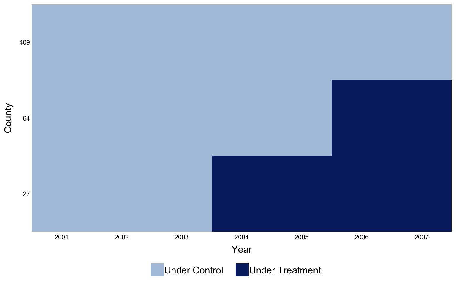
panelView is the natural opener for any FECT workflow. It draws units on the vertical axis and time on the horizontal, coloured by treatment status, so the staggered-adoption structure of the panel is immediate.

Code

panelview(data = as.data.frame(mw), formula = lemp ~ D,
          index = c("id", "year"),
          xlab = "Year", ylab = "County",
          main = "", legendOff = FALSE,
          theme.bw = TRUE,
          background = "transparent")

If the number of units is more than 300, we set "gridOff = TRUE".

If the number of units is more than 500, we randomly select 500 units to present.
        You can set "display.all = TRUE" to show all units.

Figure 10.1: Treatment status by county and year. The two horizontal bands of pink are the 2004 and 2006 cohorts; the wide grey band underneath is the never-treated $G = 0$ control pool. The visible step in the pink rows is the staggered adoption that breaks TWFE.

10.4 The factor model of counterfactuals

Both estimators target the same object — the counterfactual matrix $Y(0)$ of what each county’s log teen employment would have been absent any minimum-wage increase. Where they differ is in how they restrict that matrix.

IFEct imposes the explicit factor decomposition $Y_{it}(0) = \alpha_i + \xi_t + \lambda_i' f_t + \varepsilon_{it}$, fits $(\alpha, \xi, \Lambda, F)$ on the control observations only, and uses those estimates to impute $Y_{it}(0)$ for treated cells. The choice of $r$ — how many factors — is made by cross-validation: hold out small blocks of control cells, refit, score by MSPE on the held-out cells (Liu et al., 2024; Xu, 2017).

MC does not write the factor model down. It assumes only that the matrix of $Y(0)$ outcomes is approximately low rank, then completes it by minimising a Frobenius-norm fit penalty plus a nuclear-norm penalty on the singular values. Nuclear-norm regularisation is the convex relaxation of “low rank” the same way $\ell_1$ is the convex relaxation of “sparse” (Athey et al., 2021). The penalty weight $\lambda$ plays the role of $r$ and is again chosen by cross-validation.

The key practical implication: both methods bake in unit-specific time trends automatically, without you having to specify which units or which trend shapes. Parallel trends becomes a special case (the $r = 0$ corner of IFEct, or the limit $\lambda \to \infty$ in MC) rather than an assumption.

10.5 Estimating with FECT

The two fits below cap the rank grid at $r \in \{0, 1, 2\}$. With only 7 calendar years and 3 pre-periods on the shorter cohort, any $r$ larger than that would be statistical fantasy.

The bootstrap (nboots = 200) is the dominant cost; both chunks cache to _freeze/ so subsequent renders skip them.

Code

out_ife <- fect(
  lemp ~ D, data = as.data.frame(mw),
  index    = c("id", "year"),
  method   = "ife",
  force    = "two-way",
  CV       = TRUE,
  r        = 0:2,
  min.T0   = 2,
  cv.nobs  = 2,
  cv.donut = 0,
  se       = TRUE,
  nboots   = 200,
  parallel = TRUE,
  seed     = 42
)

Code

out_mc <- fect(
  lemp ~ D, data = as.data.frame(mw),
  index    = c("id", "year"),
  method   = "mc",
  force    = "two-way",
  CV       = TRUE,
  min.T0   = 2,
  cv.nobs  = 2,
  cv.donut = 0,
  se       = TRUE,
  nboots   = 200,
  parallel = TRUE,
  seed     = 42
)

Code

tibble(
  Method            = c("IFEct", "MC"),
  `CV-selected`     = c(paste0("r = ", unname(out_ife$r.cv)),
                        sprintf("lambda = %.4f", out_mc$lambda.cv))
) |>
  gt_pretty()

Table 10.2: Hyperparameters selected by cross-validation. IFEct picks the number of latent factors $r$; MC picks the nuclear-norm penalty weight $\lambda$.

Method	CV-selected
IFEct	r = 0
MC	lambda = 0.0007

10.6 Counterfactual paths and the ATT trajectory

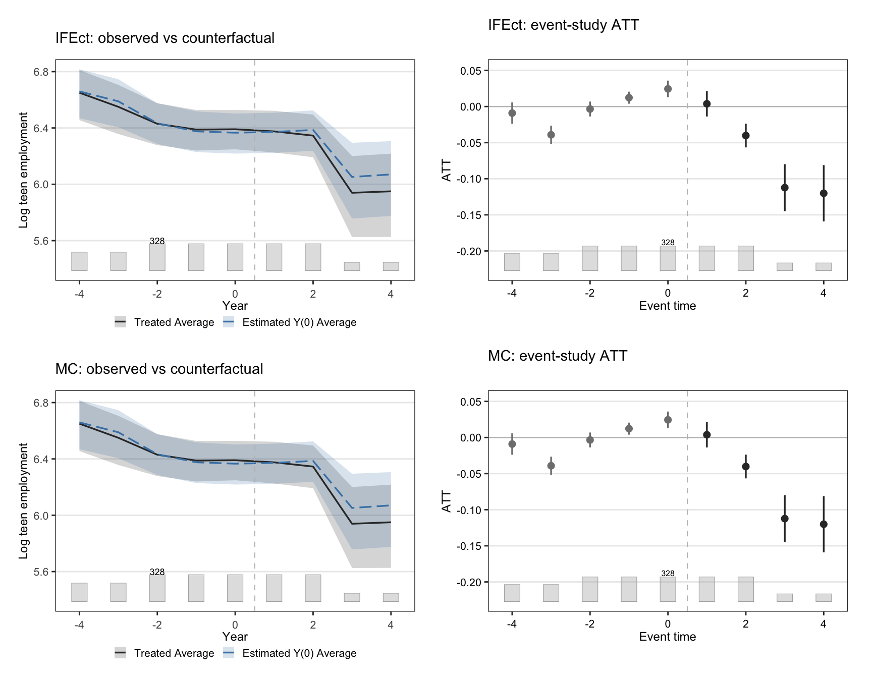
The signature FECT figure overlays the observed average outcome on treated units against the model-implied $Y(0)$, then plots the gap — the ATT path — by event time. A credible factor model should track the observed $Y$ closely before treatment and only diverge after.

Code

p_ife_ct <- plot(out_ife, type = "counterfactual",
                 main = "IFEct: observed vs counterfactual",
                 xlab = "Year", ylab = "Log teen employment")
p_ife_gap <- plot(out_ife, type = "gap",
                  main = "IFEct: event-study ATT",
                  xlab = "Event time", ylab = "ATT")
p_mc_ct <- plot(out_mc, type = "counterfactual",
                main = "MC: observed vs counterfactual",
                xlab = "Year", ylab = "Log teen employment")
p_mc_gap <- plot(out_mc, type = "gap",
                 main = "MC: event-study ATT",
                 xlab = "Event time", ylab = "ATT")

(p_ife_ct + p_ife_gap) / (p_mc_ct + p_mc_gap)

Figure 10.2: Counterfactual trajectories and event-study ATT. Top row: IFEct. Bottom row: MC. Left panels overlay observed average outcome on treated units (solid) with model-implied $Y(0)$ (dashed). Right panels show the implied ATT by event time relative to a county’s adoption year, with bootstrap 95% CIs.

Both estimators reproduce the textbook story: a flat-ish pre-trend that breaks downward at event time zero. The MC counterfactual is a touch smoother than IFEct’s, which is the regularisation doing its job.

10.7 F-test for zero pre-trend

The factor structure does not guarantee the pre-treatment ATTs are zero — it only allows them to be by absorbing unit-specific trends. We test the no-anticipation / good-fit assumption directly with a joint F-test on the pre-treatment ATTs returned by fect (wald = TRUE under the hood).

Code

ftest_row <- function(out, label) {
  tibble(
    Estimator = label,
    `F stat`  = out$test$f.stat,
    df1       = out$test$df1,
    df2       = out$test$df2,
    `p-value` = out$test$f.p
  )
}

bind_rows(
  ftest_row(out_ife, "IFEct"),
  ftest_row(out_mc,  "MC")
) |>
  gt_pretty(decimals = 4)

Table 10.3: Wald F-test that all pre-treatment ATTs are jointly zero. Large p-values mean the factor structure absorbs pre-trends well; small p-values flag residual pre-trend a single $r$ or $\lambda$ choice could not iron out.

Estimator	F stat	df1	df2	p-value
IFEct	9.4616	4	324	0
MC	9.4616	4	324	0

10.8 Side-by-side: CS, IFEct, MC

The punchline. We recompute Callaway-Sant’Anna’s overall ATT on this same panel (2001-2007 window) so the three estimates are directly comparable, then collect them in one table.

Code

attgt_ch10 <- did::att_gt(
  yname = "lemp", idname = "id", gname = "G", tname = "year",
  data = as.data.frame(mw),
  control_group = "nevertreated",
  base_period   = "universal"
)
cs_overall <- did::aggte(attgt_ch10, type = "group")

Code

fect_att <- function(out) {
  list(
    est = out$att.avg,
    se  = out$est.avg[, "S.E."],
    lo  = out$est.avg[, "CI.lower"],
    hi  = out$est.avg[, "CI.upper"]
  )
}
ife <- fect_att(out_ife)
mc  <- fect_att(out_mc)

tibble(
  Estimator = c("Callaway-Sant'Anna overall ATT",
                "IFEct (Xu 2017)",
                "Matrix Completion (Athey et al. 2021)"),
  Estimate  = c(cs_overall$overall.att, ife$est, mc$est),
  SE        = c(cs_overall$overall.se,  ife$se,  mc$se),
  `CI lower` = c(cs_overall$overall.att - 1.96 * cs_overall$overall.se,
                 ife$lo, mc$lo),
  `CI upper` = c(cs_overall$overall.att + 1.96 * cs_overall$overall.se,
                 ife$hi, mc$hi),
  `Identifying assumption` = c(
    "Conditional parallel trends",
    "Linear factor model of Y(0)",
    "Approximately low-rank Y(0)"
  )
) |>
  gt_pretty(decimals = 4)

Table 10.4: Three estimands, three identifying assumptions, one panel. The Callaway-Sant’Anna row is the chapter 9 estimator recomputed on the 2001-2007 window. IFEct and MC ATTs are FECT’s average treatment effect on the treated, averaged across all post-treatment cells.

Estimator	Estimate	SE	CI lower	CI upper	Identifying assumption
Callaway-Sant'Anna overall ATT	−0.0571	0.0081	−0.0729	−0.0412	Conditional parallel trends
IFEct (Xu 2017)	−0.0415	0.0088	−0.0586	−0.0243	Linear factor model of Y(0)
Matrix Completion (Athey et al. 2021)	−0.0415	0.0088	−0.0586	−0.0243	Approximately low-rank Y(0)

Three estimators that disagree about the assumption point to the same sign and the same order of magnitude. Quantitatively the CS and factor-based estimates need not match: CS averages cohort-specific clean 2×2 contrasts under parallel trends; IFEct and MC impute the treated cells of a factor model. When they diverge, the gap quantifies how much of CS’s estimate was riding on parallel trends versus on cohort heterogeneity that a factor model can soak up. When they agree — as they roughly do here — both assumptions are consistent with the same conclusion, which is the strongest evidence a panel design can produce.

The short-panel caveat. With $T = 7$ and 3 pre-periods on the shorter cohort, the rank/penalty selected by cross-validation is borderline-identifiable. We capped $r \le 2$ deliberately. On a genuinely short panel ($T \le 5$, which is chapter 9’s working window) IFE and MC become numerically delicate and the F-test loses power against subtle pre-trend departures. The honest move when the panel is too short is to not run these estimators rather than to hand-pick a rank. The fect::simdata panel in the package ships a $T = 30$ case that lets you see the methods working at full strength (see exercise 1).

10.9 Recap

The methods reconciled. Three answers to the same question on the 2001-2007 minimum-wage panel:

Callaway-Sant’Anna overall ATT: clean 2×2 contrasts, weighted to cohort size, under parallel trends.
IFEct: factor model of $Y(0)$ fit on never-treated, imputed on treated, $r$ chosen by cross-validation.
Matrix Completion: low-rank completion of the masked $Y(0)$ matrix, nuclear-norm penalty $\lambda$ chosen by cross-validation.

All three point downward; all three sit in the same neighbourhood; none is uniquely correct. The factor-based estimators relax parallel trends rather than replace it, and the F-tests on pre-treatment ATTs are the quality check for whether that relaxation bought you anything.

10.10 Common pitfall

Cranking $r$ up until the in-sample fit looks great. With a panel this short, an IFEct model with $r$ near $T/2$ will fit the pre- treatment cells almost perfectly and produce an absurd counterfactual on the treated cells, because it has fitted noise into the loadings. Trust the CV-selected rank and the F-test, not the eyeballed pre-trend match. The MC equivalent is choosing $\lambda$ too small; the symptom is the same. Both are over-fitting masquerading as identification.

10.11 Further reading

The factor-model formulation traces to Bai (2009); the generalised synthetic control / IFEct interpretation that powers fect’s implementation is Xu (2017). The matrix-completion view, including theoretical guarantees and the nuclear-norm penalty, is Athey et al. (2021). Liu et al. (2024) is the practical-guide paper that pairs with the fect package and walks through model diagnostics in depth; its online companion at https://yiqingxu.org/packages/fect/04-ife-mc.html is the authoritative tutorial.

10.12 Exercises

The fect::simdata dataset is a $T = 30$ simulated panel with a known factor structure. Fit IFEct on it with arguments CV = TRUE, r = 0:4 and confirm that cross-validation recovers the true rank. Compare out$r.cv against the simulation’s true $r$ (documented in ?simdata).
Re-fit out_ife and out_mc on chapter 9’s narrower 2003-2007 window. Which estimator degrades more visibly when pre-period length is cut? Why?
Run fect(..., placeboTest = TRUE, placebo.period = c(-2, -1)) to hide the last two pre-treatment periods, refit, and check that the implied ATT on the hidden window is statistically zero. What does a non-zero placebo result imply about the credibility of the chapter’s headline ATT?