---
title: "Staggered Differences-in-Differences"
---
## When Basic DiD breaks
Chapter 4 ran a textbook 2×2 DiD on Proposition 99, with California
treated in 1989 and Nevada as the single hand-picked control. The
estimate collapsed to roughly $-5.7$ packs per capita and could not
be distinguished from zero. The diagnosis there was that Nevada is
geographically and culturally adjacent to California and absorbs the
same secular forces — so its post-1988 decline soaks up most of what
we wanted to attribute to the policy.
There is a deeper structural problem too. Real policy data rarely
has just one treated unit and one clean control unit, both treated
at the same instant. States and counties **adopt at different times**
— some in 2004, others in 2006, still others never. The natural
extension of the chapter 4 model to that setting is *two-way fixed
effects (TWFE)* regression:
$$y_{it} = \alpha_i + \gamma_t + \beta \cdot \text{post}_{it} + \varepsilon_{it}.$$
For two decades this was the default. We now know it is biased in the
presence of staggered adoption: already-treated units silently act as
*controls* for later-treated units, contaminating the contrast. The
"DiD coefficient" $\hat\beta$ becomes a weighted average of group-time
ATTs with **some negative weights** [@goodmanbacon2021difference;
@dechaisemartin2020twoway]. When treatment effects grow over time —
the textbook policy story — those negative weights can flip the sign
of $\hat\beta$ relative to any sensible average effect.
This chapter walks through the modern toolkit for repairing that
damage. The methods build on @callaway2021difference: estimate
**group-time average treatment effects** $ATT(g, t)$ directly, then
aggregate them with weights you can defend. Along the way we look
at three companion ideas: the Sun-Abraham interaction-weighted event
study [@sun2021estimating], the doubly-robust DiD estimator from
@callaway2021difference, and the Rambachan-Roth sensitivity analysis
that quantifies how much parallel-trends violation it would take to
overturn the conclusion [@rambachan2023more].
The dataset is no longer Proposition 99. Staggered DiD requires
**variation in treatment timing**, which a single-treated-state panel
cannot provide. We switch to the Callaway-Sant'Anna minimum-wage
panel: 1,745 US counties × 2003–2007, with cohorts $G \in \{0, 2004,
2006\}$ indexing the year the county's state first raised its minimum
wage above the federal $5.15/h floor. The outcome is log teen
employment.
## Setup and data
```{r}
#| label: setup
#| message: false
#| warning: false
library(tidyverse)
library(did)
library(fixest)
library(twfeweights)
library(HonestDiD)
library(DRDID)
library(BMisc)
library(pte)
library(patchwork)
source("R/table_helpers.R")
source("R/honest_did.R")

set.seed(42)

knitr::opts_chunk$set(dev.args = list(bg = "transparent"))

theme_set(
  theme_minimal(base_size = 12) +
    theme(
      plot.background  = element_rect(fill = "transparent", color = NA),
      panel.background = element_rect(fill = "transparent", color = NA),
      panel.grid.major = element_line(color = "#94a3b8", linewidth = 0.25),
      panel.grid.minor = element_line(color = "#94a3b8", linewidth = 0.15),
      text             = element_text(color = "#94a3b8"),
      axis.text        = element_text(color = "#94a3b8"),
      strip.text       = element_text(color = "#94a3b8"),
      legend.text      = element_text(color = "#94a3b8")
    )
)
```
The dataset ships as `data/cs_minwage.rds` in the chapter bundle. We
follow the source-post convention of restricting to cohorts $G \in
\{0, 2004, 2006, 2007\}$, dropping the Northeast region (`region ==
"1"`) for comparability, and then carving out a clean working panel
without the late-2007 cohort and starting in 2003.
```{r}
#| label: data-load
mw_raw <- readRDS("data/cs_minwage.rds") |> as_tibble()

# Step 1: drop Northeast and keep cohorts of interest.
mw <- mw_raw |>
  filter(G %in% c(0, 2004, 2006, 2007), region != "1")

# Step 2: working sample for the main analysis.
data2 <- mw |>
  filter(G != 2007, year >= 2003)

dim(data2)
```
The working panel has `r nrow(data2)` rows on
`r length(unique(data2$id))` counties, balanced across the
2003–2007 window.
```{r}
#| label: tbl-cohort-counts
#| tbl-cap: "Cohort sizes in the working sample. G = 0 is the never-treated control pool; cohorts 2004 and 2006 are the staggered treated groups."
data2 |>
  filter(year == 2003) |>
  count(G, name = "counties") |>
  rename(`Treatment cohort (G)` = G) |>
  gt_pretty()
```
## The TWFE baseline and its problem
The natural first move is the TWFE regression. The variable `post` in
the dataset is 1 in periods where the county's state has already
raised its minimum wage (i.e., `year >= G & G != 0`), and 0 otherwise.
```{r}
#| label: tbl-twfe
#| tbl-cap: "Two-way fixed-effects regression. The point estimate suggests minimum-wage increases cut log teen employment by roughly 3.8 percent — but see the diagnostic that follows."
twfe_res <- fixest::feols(lemp ~ post | id + year,
                          data = data2, cluster = "id")
ms_pretty(list("TWFE (county + year FE)" = twfe_res),
          coef_map = c("post" = "Post (any cohort)"),
          notes    = "SEs clustered at the county level.")
```
The TWFE coefficient is roughly $-0.038$. Read literally, the policy
reduced teen employment by 3.8 percent. Before believing it, two
diagnostics are essential.
### Sun-Abraham event study
The first is to allow the effect to *evolve* with time since treatment
— an event-study specification. The naive interacted version,
$y_{it} = \alpha_i + \gamma_t + \sum_{k \ne -1} \beta_k \cdot
\mathbf{1}(t - G_i = k) + \varepsilon_{it}$, is itself biased in
staggered designs. The @sun2021estimating fix is the interaction-
weighted estimator implemented by `fixest::sunab()`.
```{r}
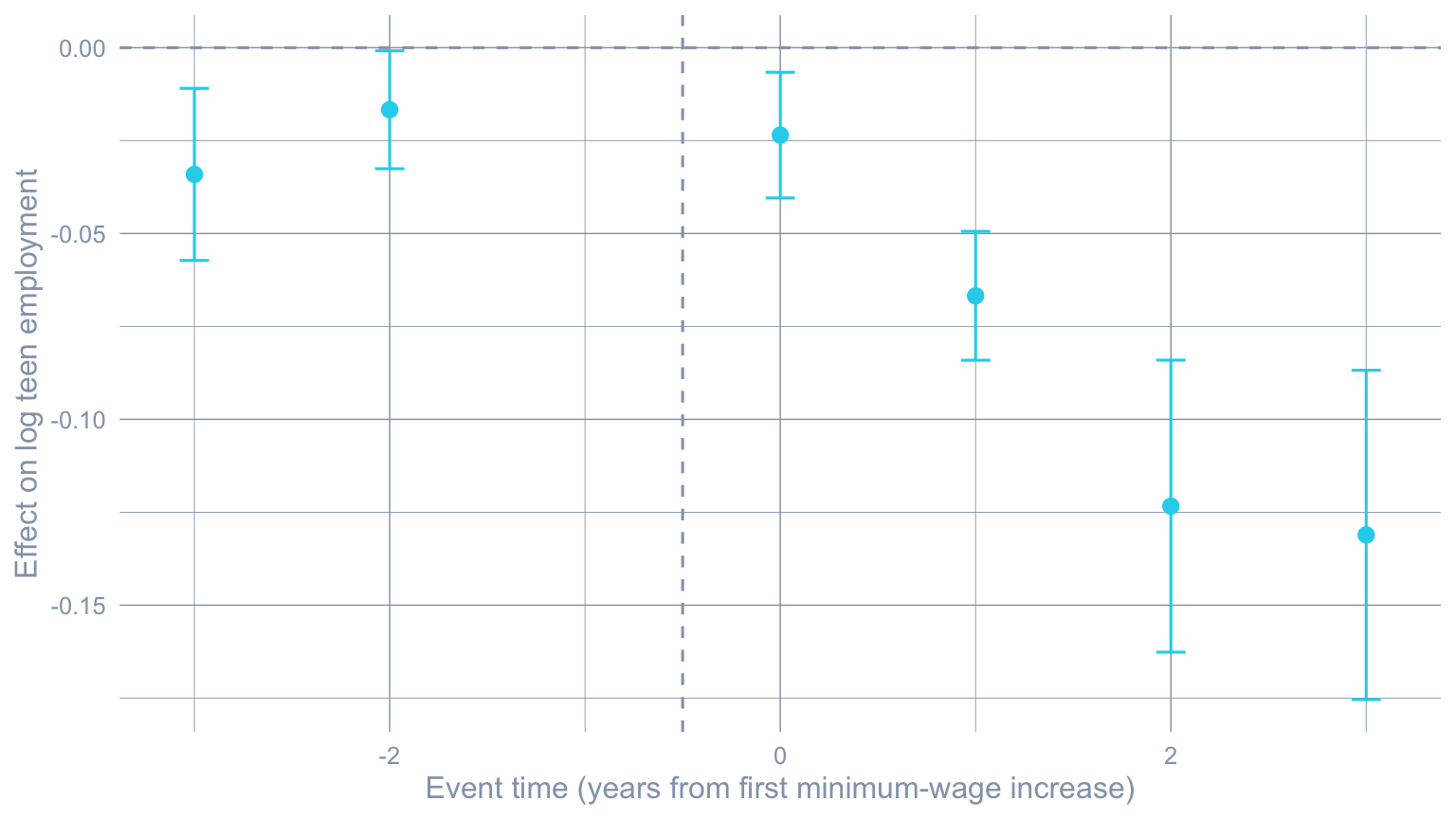
#| label: fig-sunab
#| fig-cap: "Sun-Abraham event study. Pre-treatment leads (negative event time) trend slightly below zero; post-treatment effects accumulate from -0.025 on impact to roughly -0.13 by event-time +3."
#| fig-width: 8
#| fig-height: 4.5
sa_res <- fixest::feols(lemp ~ sunab(G, year) | id + year,
                        data = data2, cluster = "id")

sa_df <- broom::tidy(sa_res, conf.int = TRUE) |>
  filter(stringr::str_detect(term, "^year::")) |>
  mutate(event_time = as.integer(stringr::str_remove(term, "^year::")))

ggplot(sa_df, aes(x = event_time, y = estimate)) +
  geom_hline(yintercept = 0, color = "#94a3b8", linetype = "dashed") +
  geom_vline(xintercept = -0.5, color = "#94a3b8", linetype = "dashed") +
  geom_point(color = "#22d3ee", size = 2.5) +
  geom_errorbar(aes(ymin = conf.low, ymax = conf.high),
                color = "#22d3ee", width = 0.15) +
  labs(x = "Event time (years from first minimum-wage increase)",
       y = "Effect on log teen employment")
```
A clean event study should show **flat pre-treatment leads near zero**,
then post-treatment effects that look credible. The Sun-Abraham
picture is mixed: a clearly negative on-impact effect that grows over
time, but pre-trends that are not perfectly flat. This is the
parallel-trends concern we will quantify with HonestDiD in section 7.
### TWFE weight decomposition
The second diagnostic asks: among the underlying group-time
comparisons that TWFE silently aggregates, **what weights does it
use?** @goodmanbacon2021difference shows that TWFE weights *can* be
negative, especially when an already-treated unit is being used as a
control for a later-treated one. `twfeweights::twfe_weights()` and
`twfeweights::attO_weights()` give us the weights TWFE actually
applies and the weights an unbiased aggregator (the @callaway2021difference
overall ATT) would apply for comparison.
```{r}
#| label: tbl-twfe-weight-summary
#| tbl-cap: "TWFE weight diagnostic. Negative or pre-treatment weights are a red flag — they mean TWFE is silently subtracting effects you would not want it to subtract."
attgt_for_weights <- did::att_gt(
  yname = "lemp", idname = "id", gname = "G", tname = "year",
  data = data2, control_group = "nevertreated",
  base_period = "universal"
)

tw <- twfeweights::twfe_weights(attgt_for_weights)
wO <- twfeweights::attO_weights(attgt_for_weights)

tw_df <- tibble(
  twfe_weight = tw$weights_df$weight,
  attO_weight = wO$weights_df$weight,
  post        = as.integer(as.character(tw$weights_df$post))
)

summary_tbl <- tibble(
  `Weight source` = c("TWFE",
                      "TWFE (pre-treatment cells)",
                      "TWFE (post-treatment cells)",
                      "ATT-O (Callaway-Sant'Anna)"),
  `Min`        = c(min(tw_df$twfe_weight),
                   min(tw_df$twfe_weight[tw_df$post == 0]),
                   min(tw_df$twfe_weight[tw_df$post == 1]),
                   min(tw_df$attO_weight)),
  `Max`        = c(max(tw_df$twfe_weight),
                   max(tw_df$twfe_weight[tw_df$post == 0]),
                   max(tw_df$twfe_weight[tw_df$post == 1]),
                   max(tw_df$attO_weight)),
  `Sum`        = c(sum(tw_df$twfe_weight),
                   sum(tw_df$twfe_weight[tw_df$post == 0]),
                   sum(tw_df$twfe_weight[tw_df$post == 1]),
                   sum(tw_df$attO_weight))
)
gt_pretty(summary_tbl, decimals = 3)
```
```{r}
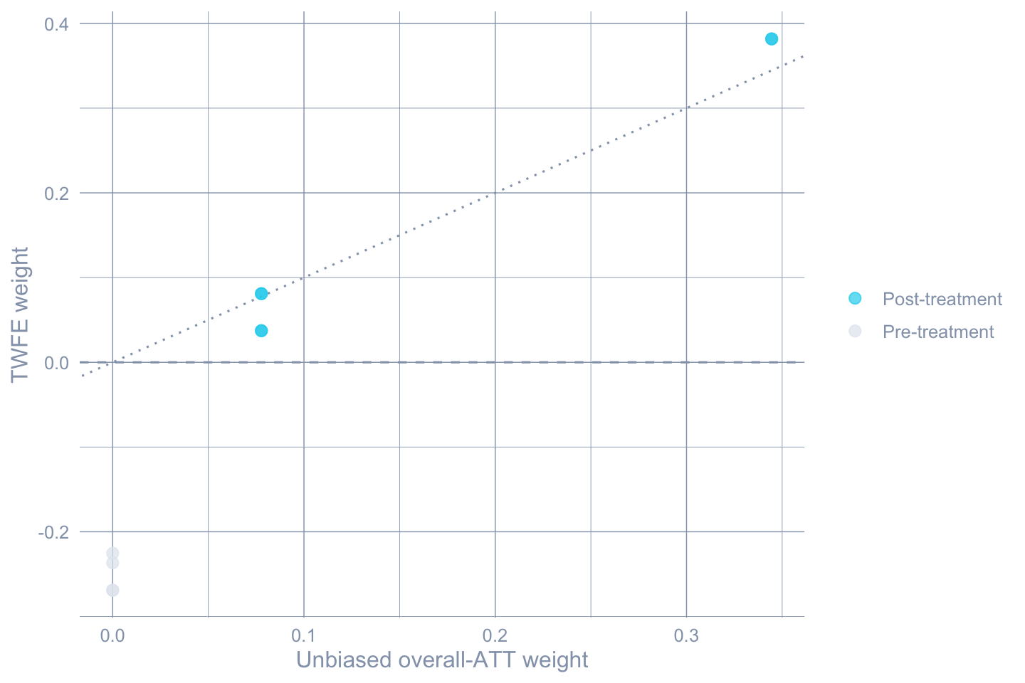
#| label: fig-twfe-weights
#| fig-cap: "TWFE vs. Callaway-Sant'Anna overall-ATT weights for the same set of group-time cells. TWFE puts non-trivial mass on pre-treatment cells (negative weights, dashed line) and weights some post-treatment cells very differently from the unbiased target."
#| fig-width: 7.5
#| fig-height: 5
tw_plot <- tw_df |>
  mutate(period = ifelse(post == 1, "Post-treatment", "Pre-treatment"))

ggplot(tw_plot, aes(x = attO_weight, y = twfe_weight, color = period)) +
  geom_hline(yintercept = 0, color = "#94a3b8", linetype = "dashed") +
  geom_abline(slope = 1, intercept = 0,
              color = "#94a3b8", linetype = "dotted") +
  geom_point(size = 2.5, alpha = 0.7) +
  scale_color_manual(values = c("Pre-treatment"  = "#e2e8f0",
                                "Post-treatment" = "#22d3ee")) +
  labs(x = "Unbiased overall-ATT weight",
       y = "TWFE weight", color = NULL)
```
The pre-treatment cells get weight from TWFE but zero weight from the
unbiased ATT-O aggregator — this is the mechanism behind
Goodman-Bacon's "contamination" diagnosis. The dotted 45-degree line
would mark perfect agreement.
## Group-time ATTs: the Callaway-Sant'Anna approach
The fix is to estimate the *primitive* objects directly. For each
cohort $g$ (a year a group of counties was first treated) and each
calendar year $t$, define
$$ATT(g, t) = \mathbb{E}\!\left[Y_{it}(g) - Y_{it}(\infty) \mid G_i = g\right],$$
the average effect on cohort $g$ in year $t$ relative to its own
never-treated potential outcome. `did::att_gt()` estimates each of
these from a clean 2×2 DiD using only cohort $g$ and an appropriate
comparison group (here, the never-treated $G = 0$), so no
contamination from already-treated units sneaks in.
```{r}
#| label: tbl-attgt
#| tbl-cap: "Group-time average treatment effects $ATT(g, t)$ for the minimum-wage panel. Cohorts 2004 and 2006, each year 2003 through 2007. Pre-treatment cells should hover near zero if parallel trends holds; post-treatment cells are the effects we want."
attgt <- did::att_gt(yname = "lemp", idname = "id", gname = "G",
                     tname = "year", data = data2,
                     control_group = "nevertreated",
                     base_period = "universal")

attgt_df <- tibble(
  Cohort       = attgt$group,
  Year         = attgt$t,
  `ATT(g,t)`   = attgt$att,
  SE           = as.numeric(attgt$se)
) |>
  mutate(`Treated?` = ifelse(Year >= Cohort, "post", "pre")) |>
  arrange(Cohort, Year)

gt_pretty(attgt_df, decimals = 4)
```
### Aggregation: overall ATT and event study
The 8 cells in @tbl-attgt are the primitives. They are not the
headline. Aggregating them produces summaries that are valid in the
presence of staggered adoption.
The **overall ATT** weights each post-treatment $ATT(g, t)$ by the
size of cohort $g$, then averages within cohort and over cohorts. It
answers: *across treated counties and across the time they had been
treated for, what is the average effect?*
```{r}
#| label: tbl-cs-overall
#| tbl-cap: "Callaway-Sant'Anna overall ATT (sample-weighted aggregation across cohorts). This is the staggered-DiD analogue of chapter 4's single DiD coefficient."
attO <- did::aggte(attgt, type = "group")

tibble(
  Estimator             = "Callaway-Sant'Anna overall ATT",
  `Estimate`            = attO$overall.att,
  `SE`                  = attO$overall.se,
  `CI lower`            = attO$overall.att - 1.96 * attO$overall.se,
  `CI upper`            = attO$overall.att + 1.96 * attO$overall.se
) |> gt_pretty(decimals = 4)
```
The overall ATT is roughly $-0.057$ — almost 50 percent larger in
magnitude than the TWFE coefficient. The two estimands answer
different questions, but the size of the gap is exactly the
contamination problem in operation.
The **event-study aggregation** averages $ATT(g, t)$ within each
event time $e = t - g$, giving a curve of dynamic effects since
treatment.
```{r}
#| label: tbl-cs-event
#| tbl-cap: "Callaway-Sant'Anna event-study aggregation. Event time -1 is the omitted reference period under the universal base."
attes <- did::aggte(attgt, type = "dynamic")

tibble(
  `Event time` = attes$egt,
  `ATT(e)`     = attes$att.egt,
  SE           = attes$se.egt,
  `CI lower`   = attes$att.egt - 1.96 * attes$se.egt,
  `CI upper`   = attes$att.egt + 1.96 * attes$se.egt
) |> gt_pretty(decimals = 4)
```
```{r}
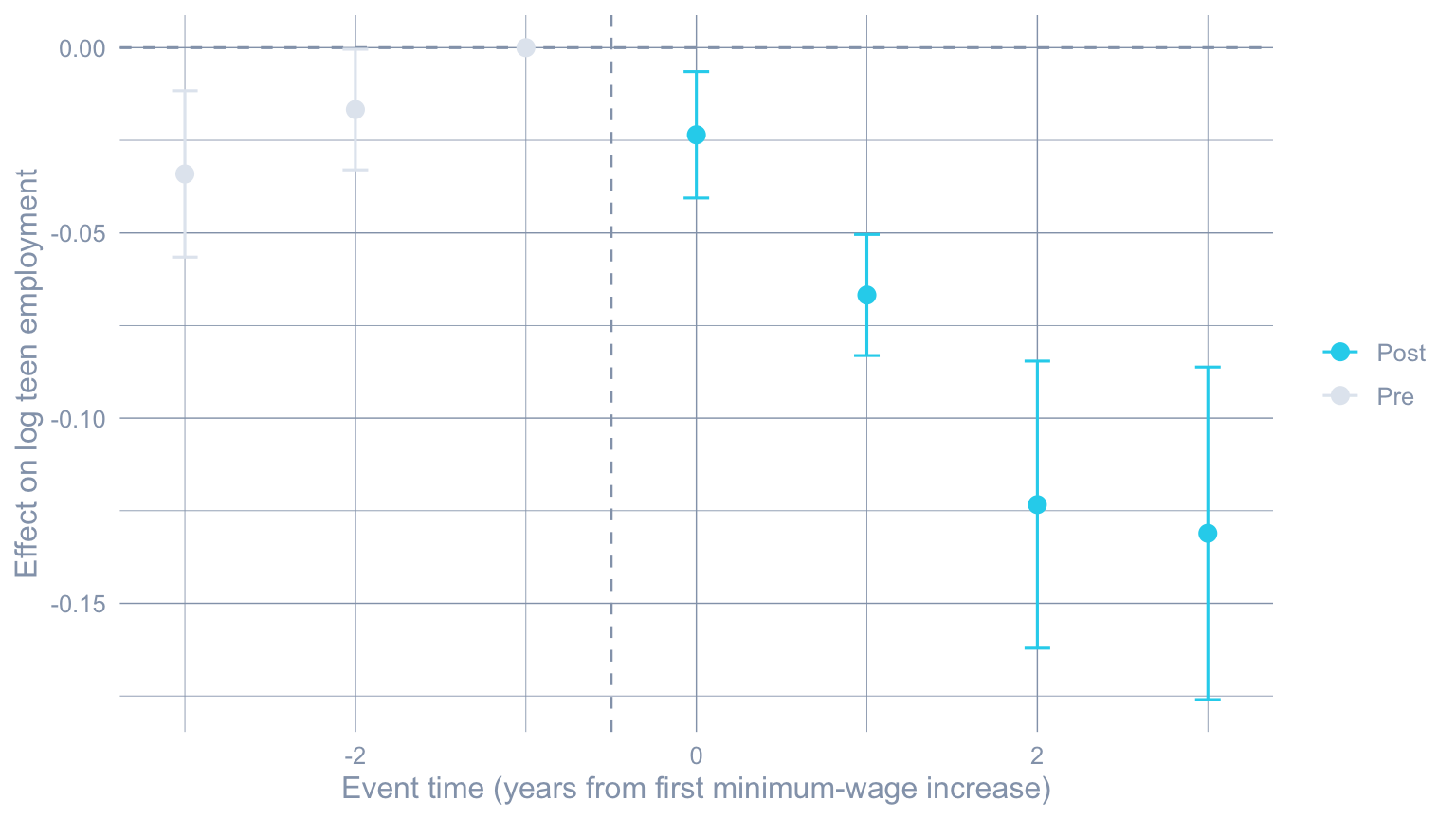
#| label: fig-cs-event
#| fig-cap: "Callaway-Sant'Anna event study. The on-impact effect is small; effects accumulate to roughly -0.13 log points by event-time +3 (three years post-treatment)."
#| fig-width: 8
#| fig-height: 4.5
cs_es_df <- tibble(
  egt   = attes$egt,
  est   = attes$att.egt,
  se    = attes$se.egt,
  phase = ifelse(attes$egt < 0, "Pre", "Post")
)

ggplot(cs_es_df, aes(x = egt, y = est, color = phase)) +
  geom_hline(yintercept = 0, color = "#94a3b8", linetype = "dashed") +
  geom_vline(xintercept = -0.5, color = "#94a3b8", linetype = "dashed") +
  geom_point(size = 2.8) +
  geom_errorbar(aes(ymin = est - 1.96 * se, ymax = est + 1.96 * se),
                width = 0.15) +
  scale_color_manual(values = c("Pre"  = "#e2e8f0",
                                "Post" = "#22d3ee")) +
  labs(x = "Event time (years from first minimum-wage increase)",
       y = "Effect on log teen employment", color = NULL)
```
## Conditional parallel trends
Plain DiD assumes parallel trends *unconditionally*. Conditional DiD
allows trends to be parallel only after adjusting for observed
covariates that shape the trajectory. In this dataset, log county
population and log average county pay are obvious candidates: counties
with bigger populations or higher-paying jobs may move on different
underlying trajectories whether or not they raise the minimum wage.
`did::att_gt()` accepts `xformla = ~lpop + lavg_pay` plus a choice of
estimator: **regression adjustment** (impute the counterfactual mean
from the never-treated), **inverse probability weighting** (reweight
never-treated counties to look like treated ones), or **doubly
robust** (the @callaway2021difference default, which is consistent
if either the outcome model *or* the propensity score is correctly
specified).
```{r}
#| label: tbl-conditional
#| tbl-cap: "Overall ATT under four identification assumptions: unconditional parallel trends, regression adjustment, inverse probability weighting, and doubly robust. The four point estimates land within roughly one SE of each other, which is reassuring."
#| message: false
#| warning: false
cs_reg <- did::att_gt(yname="lemp", tname="year", idname="id", gname="G",
                      xformla = ~lpop + lavg_pay,
                      control_group = "nevertreated",
                      base_period = "universal",
                      est_method = "reg", data = data2)
attO_reg <- did::aggte(cs_reg, type = "group")

cs_ipw <- did::att_gt(yname="lemp", tname="year", idname="id", gname="G",
                      xformla = ~lpop + lavg_pay,
                      control_group = "nevertreated",
                      base_period = "universal",
                      est_method = "ipw", data = data2)
attO_ipw <- did::aggte(cs_ipw, type = "group")

cs_dr  <- did::att_gt(yname="lemp", tname="year", idname="id", gname="G",
                      xformla = ~lpop + lavg_pay,
                      control_group = "nevertreated",
                      base_period = "universal",
                      est_method = "dr", data = data2)
attO_dr  <- did::aggte(cs_dr, type = "group")

tibble(
  Identification = c("Unconditional parallel trends",
                     "Conditional · regression adjustment",
                     "Conditional · IPW",
                     "Conditional · doubly robust"),
  Estimate = c(attO$overall.att, attO_reg$overall.att,
               attO_ipw$overall.att, attO_dr$overall.att),
  SE       = c(attO$overall.se,  attO_reg$overall.se,
               attO_ipw$overall.se,  attO_dr$overall.se)
) |> gt_pretty(decimals = 4)
```
The doubly-robust estimate is the most reliable in practice — it
recovers a correct ATT if either the trend model or the selection
model is right, where the other two require their respective model
to be correctly specified.
## Robustness knobs
Three knobs are worth turning to gauge how fragile the headline
estimate is to design choices.
```{r}
#| label: tbl-robustness
#| tbl-cap: "Overall ATT under three robustness perturbations: shifting from a universal to a varying base period, switching the control group from never-treated to not-yet-treated, and allowing one year of anticipation."
#| message: false
#| warning: false
cs_var <- did::att_gt(yname="lemp", tname="year", idname="id", gname="G",
                      xformla = ~lpop + lavg_pay,
                      control_group = "nevertreated",
                      base_period = "varying",
                      est_method = "dr", data = data2)
attO_var <- did::aggte(cs_var, type = "group")

cs_nyt <- did::att_gt(yname="lemp", tname="year", idname="id", gname="G",
                      xformla = ~lpop + lavg_pay,
                      control_group = "notyettreated",
                      base_period = "universal",
                      est_method = "dr", data = data2)
attO_nyt <- did::aggte(cs_nyt, type = "group")

cs_ant <- did::att_gt(yname="lemp", tname="year", idname="id", gname="G",
                      xformla = ~lpop + lavg_pay,
                      control_group = "nevertreated",
                      base_period = "universal",
                      est_method = "dr",
                      anticipation = 1, data = data2)
attO_ant <- did::aggte(cs_ant, type = "group")

tibble(
  Specification = c("Doubly robust (baseline)",
                    "Varying base period",
                    "Not-yet-treated controls",
                    "Anticipation = 1 year"),
  Estimate = c(attO_dr$overall.att, attO_var$overall.att,
               attO_nyt$overall.att, attO_ant$overall.att),
  SE       = c(attO_dr$overall.se,  attO_var$overall.se,
               attO_nyt$overall.se,  attO_ant$overall.se)
) |> gt_pretty(decimals = 4)
```
None of the robustness checks moves the estimate by more than its own
standard error. That is the strongest internal evidence we have that
the design is identifying a stable effect.
## Sensitivity to parallel-trends violations
The robustness table only varies *design* choices; it does not
quantify *how much* parallel trends would have to be violated to
overturn the conclusion. @rambachan2023more provide exactly that
quantification. The `HonestDiD` package, paired with a small bridge
function in `R/honest_did.R`, lets us bound the post-treatment effect
under the assumption that any unobserved pre-trend violation is at
most $\bar M$ times the largest *observed* pre-trend violation.
```{r}
#| label: tbl-honest
#| tbl-cap: "Robust confidence intervals for the on-impact effect $ATT(e = 0)$ under the relative-magnitude restriction. As $\\bar M$ grows, the CI widens; we report the breakdown point — the $\\bar M$ at which the CI first contains zero."
#| message: false
#| warning: false
attgt_hd <- did::att_gt(yname="lemp", idname="id", gname="G",
                        tname="year", data=data2,
                        control_group="nevertreated",
                        base_period="universal")
cs_es_hd <- did::aggte(attgt_hd, type="dynamic")

hd_rm <- honest_did(es      = cs_es_hd,
                    e       = 0,
                    type    = "relative_magnitude",
                    method  = "C-LF",
                    Mbarvec = seq(0, 2, by = 0.5))

hd_rm |>
  transmute(`$\\bar M$` = Mbar,
            `CI lower`  = lb,
            `CI upper`  = ub,
            `Contains 0?` = ifelse(lb <= 0 & 0 <= ub, "yes", "no")) |>
  gt_pretty(decimals = 4)
```
```{r}
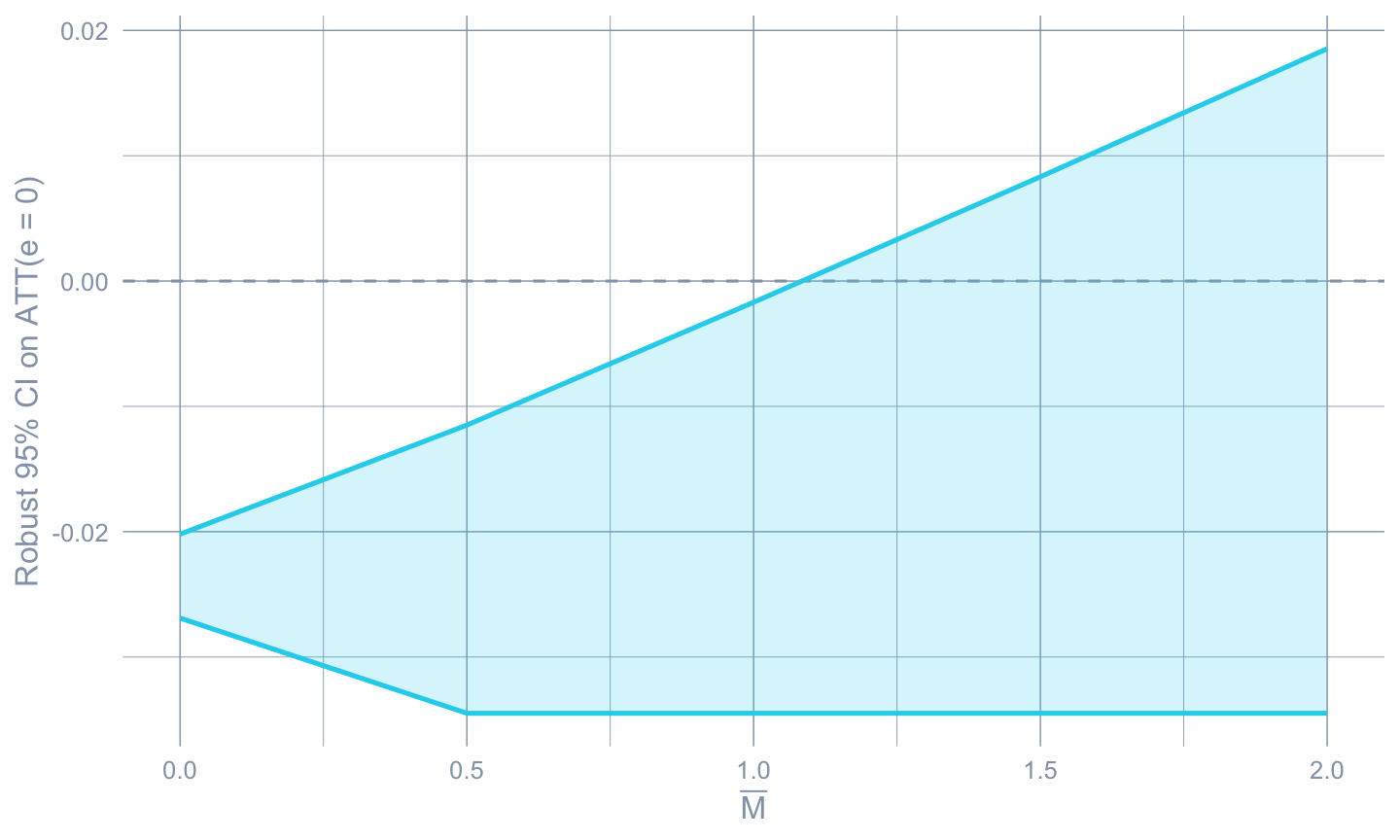
#| label: fig-honest
#| fig-cap: "HonestDiD sensitivity: as $\\bar M$ grows, the robust 95 percent CI on the on-impact effect widens until it crosses zero. The breakdown $\\bar M$ is roughly 1; effects of the magnitude observed in the data survive any pre-trend violation up to that size."
#| fig-width: 7.5
#| fig-height: 4.5
ggplot(hd_rm, aes(x = Mbar)) +
  geom_hline(yintercept = 0, color = "#94a3b8", linetype = "dashed") +
  geom_ribbon(aes(ymin = lb, ymax = ub),
              fill = "#22d3ee", alpha = 0.2) +
  geom_line(aes(y = lb), color = "#22d3ee", linewidth = 0.9) +
  geom_line(aes(y = ub), color = "#22d3ee", linewidth = 0.9) +
  labs(x = expression(bar(M)),
       y = "Robust 95% CI on ATT(e = 0)")
```
The breakdown point is around $\bar M \approx 1$ — meaning the
conclusion that minimum-wage increases reduce on-impact teen
employment survives any unobserved pre-trend violation up to roughly
the *largest observed pre-trend in the data*. That is a strong
robustness result.
## Heterogeneous treatment doses
State minimum wages were not raised by the same amount. Some states
went to $5.50/h, others to $7.25/h. A natural refinement is to
**normalize** each treated state's effect by the size of the wage
increase — an "ATT per dollar above the federal floor".
We follow the source post in expanding the working sample to include
the 2007 cohort (gives us more treated states and more variation in
the dose) and applying `DRDID::drdid_panel()` cell by cell on the
cohort-by-period contrasts, then dividing by the wage delta.
```{r}
#| label: dose-compute
#| message: false
#| warning: false
data3 <- mw |>
  filter(year >= 2003)
treated_state_list <- unique(subset(data3, G != 0)$state_name)

attlist <- list()
for (state in treated_state_list) {
  g <- unique(subset(data3, state_name == state)$G)
  for (period in 2004:2007) {
    if (period < g) next  # only post-treatment cells

    treat_idx_post  <- data3$state_name == state & data3$year == period
    treat_idx_base  <- data3$state_name == state & data3$year == g - 1
    if (sum(treat_idx_post) == 0 || sum(treat_idx_base) == 0) next

    ctrl_idx_post  <- data3$G == 0 & data3$year == period
    ctrl_idx_base  <- data3$G == 0 & data3$year == g - 1

    Y1 <- c(data3$lemp[treat_idx_post], data3$lemp[ctrl_idx_post])
    Y0 <- c(data3$lemp[treat_idx_base], data3$lemp[ctrl_idx_base])
    D  <- c(rep(1, sum(treat_idx_post)), rep(0, sum(ctrl_idx_post)))

    out <- DRDID::drdid_panel(y1 = Y1, y0 = Y0, D = D, covariates = NULL)
    dose <- unique(data3$state_mw[treat_idx_post]) - 5.15

    attlist[[paste(state, period, sep = "_")]] <- tibble(
      state         = state,
      cohort        = g,
      event_time    = period - g,
      att           = out$ATT,
      se            = out$se,
      dose          = dose,
      att_per_dollar = out$ATT / dose
    )
  }
}

dose_df <- bind_rows(attlist)
dose_summary <- dose_df |>
  group_by(event_time) |>
  summarise(att_per_dollar_mean = mean(att_per_dollar),
            att_per_dollar_sd   = sd(att_per_dollar),
            n                   = n(),
            .groups = "drop")
```
```{r}
#| label: tbl-dose
#| tbl-cap: "ATT per dollar of minimum-wage increase, averaged over treated states within each post-treatment event time. Effects grow with time since treatment."
dose_summary |>
  rename(`Event time`       = event_time,
         `ATT per $ (mean)` = att_per_dollar_mean,
         `ATT per $ (SD)`   = att_per_dollar_sd,
         `# states`         = n) |>
  gt_pretty(decimals = 4)
```
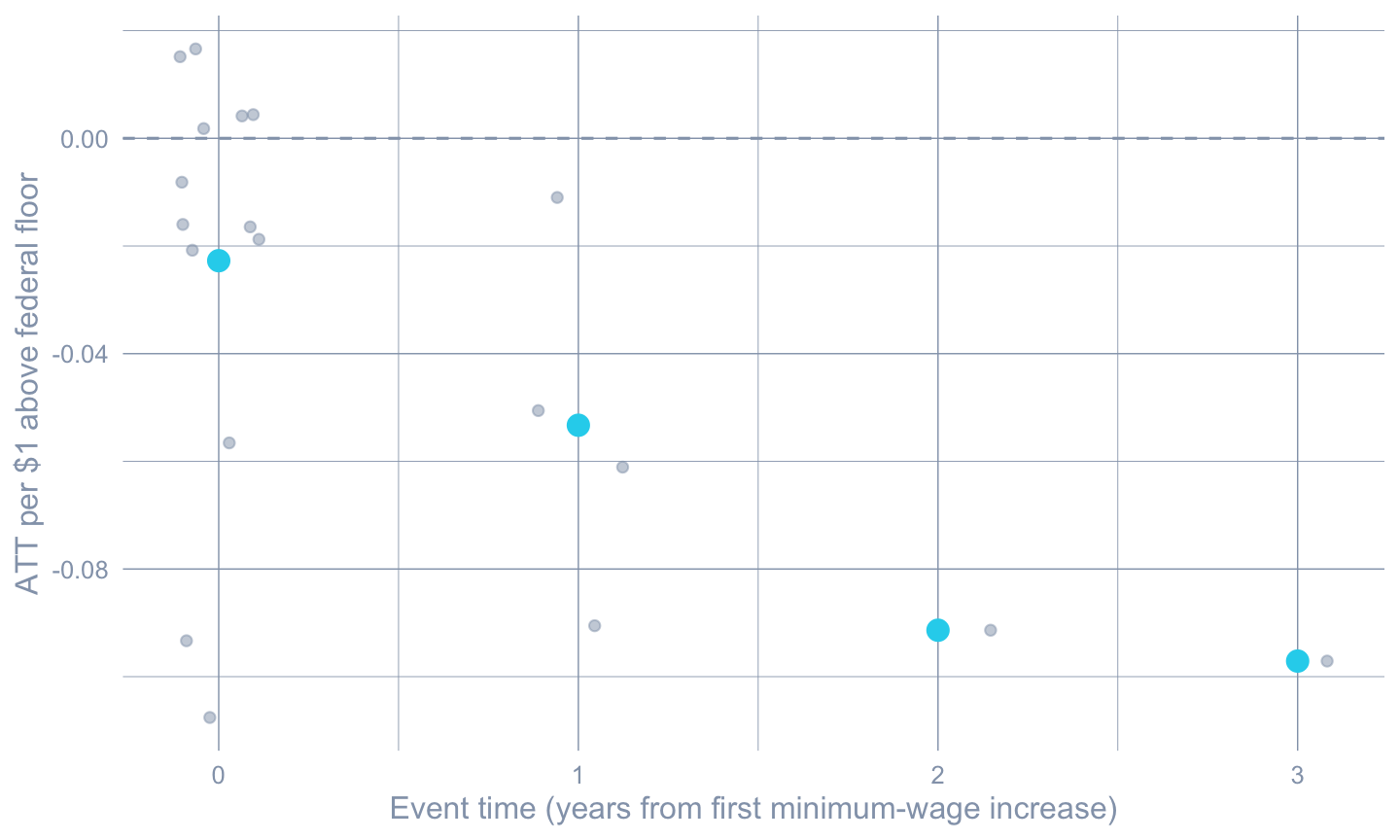
```{r}
#| label: fig-dose
#| fig-cap: "ATT per dollar of minimum-wage increase by event time. Each grey point is a (state, event-time) cell; cyan points are the cross-state means at each event time."
#| fig-width: 7.5
#| fig-height: 4.5
ggplot(dose_df, aes(x = event_time, y = att_per_dollar)) +
  geom_hline(yintercept = 0, color = "#94a3b8", linetype = "dashed") +
  geom_jitter(width = 0.15, height = 0, alpha = 0.5, color = "#94a3b8") +
  stat_summary(fun = mean, geom = "point",
               color = "#22d3ee", size = 3.5) +
  labs(x = "Event time (years from first minimum-wage increase)",
       y = "ATT per $1 above federal floor")
```
## Lagged outcomes: an alternative identifying assumption
So far every estimator relied on **parallel trends** (conditional or
unconditional). A different identifying assumption, popular in labor
economics, is that *conditional on the lagged outcome*, treatment
assignment is as good as random — the so-called **lagged-outcomes** or
**unconfoundedness on past Y** strategy. The `pte` package implements
this in the same group-time-aggregation framework as `did`.
```{r}
#| label: tbl-pte
#| tbl-cap: "Event-study estimates under the lagged-outcomes identifying assumption (pte::pte_default). The conditioning is on lagged log teen employment rather than on the parallel-trends assumption."
#| message: false
#| warning: false
data2_lo <- data2 |>
  mutate(G2 = G)

lo_res <- pte::pte_default(yname = "lemp", tname = "year", idname = "id",
                           gname = "G2", data = as.data.frame(data2_lo),
                           d_outcome = FALSE, lagged_outcome_cov = TRUE)

tibble(
  `Event time` = lo_res$event_study$egt,
  `ATT(e)`     = lo_res$event_study$att.egt,
  SE           = lo_res$event_study$se.egt
) |> gt_pretty(decimals = 4)
```
The lagged-outcomes estimate of the overall negative effect is
qualitatively similar to the parallel-trends-based estimates. Two
very different identifying assumptions point to the same substantive
conclusion — which is the strongest possible evidence the design
generates.
## Recap
::: {.callout-note appearance="simple"}
**The methods reconciled.** TWFE on this dataset returned
$\hat\beta = -0.038$. The Callaway-Sant'Anna overall ATT is
$-0.057$. The doubly-robust conditional ATT is $-0.065$. The
event-study trajectory is $\approx -0.024$ on impact, dropping to
$\approx -0.13$ by event-time $+3$. HonestDiD sensitivity puts the
breakdown $\bar M$ near 1.0. The lagged-outcomes estimator agrees in
sign and magnitude. Five very different estimators tell the same
story: *minimum-wage increases reduced teen employment in these
counties, and the effect grew over time*.
The gap between the TWFE estimate and the modern aggregators is the
contamination problem of @goodmanbacon2021difference made concrete.
TWFE absorbs $\sim 36$ percent of its weight into pre-treatment cells
and post-treatment cells with negative weights — both of which the
unbiased Callaway-Sant'Anna aggregator avoids.
:::
## Common pitfall
Running TWFE on staggered data and reporting the coefficient as if
it were a clean ATT. The bias is mechanical — already-treated units
get used as controls for later-treated units, and treatment-effect
heterogeneity over time then leaks into the coefficient with
unintended signs. **What to do instead.** Estimate the
$\{ATT(g, t)\}$ primitives directly with `did::att_gt()`, look at
the cells, and only then aggregate with `aggte()` using a target
that matches the question you actually want to answer. If you must
run TWFE for a referee, run `twfeweights::twfe_weights()` and
report the share of weight on pre-treatment cells.
## Further reading
The Callaway-Sant'Anna framework, the Goodman-Bacon decomposition,
and the Sun-Abraham interaction-weighted estimator are the three
modern reference points for staggered DiD
[@callaway2021difference; @goodmanbacon2021difference;
@sun2021estimating]. The `did` package vignettes
(<https://bcallaway11.github.io/did/>) are the canonical
implementation reference. For sensitivity analysis, the
@rambachan2023more paper plus the `HonestDiD` package documentation
cover both the smoothness and relative-magnitude bounds.
@dechaisemartin2020twoway is the parallel critique of TWFE from the
`DIDmultiplegt` perspective. @callaway2022handbook is a textbook-level
synthesis.
For a longer R walkthrough that this chapter is adapted from, see
the companion post at
<https://cmg777.github.io/post/r_did/>.
## Exercises
1. Re-estimate the overall ATT using `control_group = "notyettreated"`
instead of `"nevertreated"`. Does the answer change? Explain why
the standard error usually *shrinks* under this alternative.
2. Use `did::aggte(attgt, type = "calendar")` to aggregate by
*calendar year* rather than event time. Which calendar year shows
the largest treatment effect, and what substantive story does that
suggest?
3. Run `HonestDiD` with `type = "smoothness"` instead of
`"relative_magnitude"`, supplying `Mvec = seq(0, 0.05, by = 0.01)`.
What does the breakdown $M$ say about the credibility of the
parallel-trends assumption in this dataset?