3. The Sample Mean

metricsAI: An Introduction to Econometrics with Python and AI in the Cloud

This notebook provides an interactive introduction to one of the most important concepts in statistics: the sampling distribution of the sample mean. You’ll explore how sample means behave through experiments and simulations, building intuition for the Central Limit Theorem. All code runs directly in Google Colab without any local setup.

🎬 AI Video ✨ AI Slides 📊 Cameron Slides ✏️ Quiz 🤖 AI Tutor

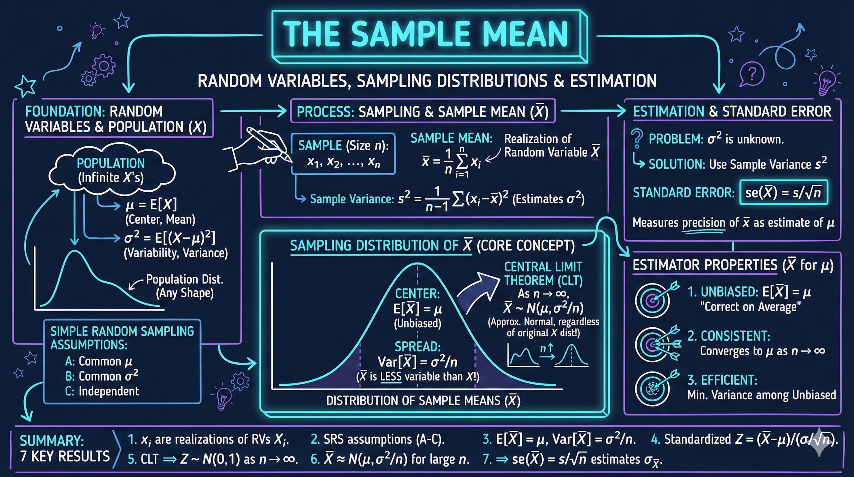
Chapter Overview

This chapter bridges the gap between descriptive statistics (Chapter 2) and inferential statistics (Chapter 4). The key insight: when we calculate a sample mean $\bar{x}$ from data, we’re observing one realization of a random variable $\bar{X}$ that has its own probability distribution.

What you’ll learn:

Understand sample values as realizations of random variables
Derive the mean and variance of the sample mean: $E[\bar{X}] = \mu$, $Var[\bar{X}] = \sigma^2/n$
Explore the sampling distribution of $\bar{X}$ through experiments
Discover the Central Limit Theorem: $\bar{X}$ is approximately normal for large $n$
Learn properties of good estimators (unbiasedness, efficiency, consistency)
Compute the standard error of the mean: $se(\bar{X}) = s/\sqrt{n}$

Datasets used:

AED_COINTOSSMEANS.DTA: 400 sample means from coin toss experiments (n=30 each)
AED_CENSUSAGEMEANS.DTA: 100 sample means from 1880 U.S. Census ages (n=25 each)

Key economic relevance: This chapter provides the theoretical foundation for ALL statistical inference in economics. Whether estimating average income, unemployment rates, or regression coefficients, understanding the sampling distribution of $\bar{X}$ is essential.

Chapter outline:

3.1 Random Variables
3.2 Experiment - Single Sample of Coin Tosses
3.3 Properties of the Sample Mean
3.4 Real Data Example - 1880 U.S. Census
3.5 Estimator Properties
3.6 Computer Simulation of Random Samples
3.7 Samples other than Simple Random Samples

Setup

First, we import the necessary Python packages and configure the environment for reproducibility. All data will stream directly from GitHub.

Setup: Import libraries and configure environment

# --- Libraries ---
import numpy as np                        # numerical operations
import pandas as pd                       # data manipulation
import matplotlib.pyplot as plt           # plotting
import seaborn as sns                     # statistical visualizations
from scipy import stats                   # statistical functions
import random
import os

# --- Reproducibility ---
RANDOM_SEED = 42
random.seed(RANDOM_SEED)
np.random.seed(RANDOM_SEED)
os.environ['PYTHONHASHSEED'] = str(RANDOM_SEED)

# --- Data source ---
GITHUB_DATA_URL = "https://raw.githubusercontent.com/quarcs-lab/data-open/master/AED/"

# --- Plotting style ---
plt.style.use('dark_background')
sns.set_style("darkgrid")
plt.rcParams.update({
    'axes.facecolor': '#1a2235',
    'figure.facecolor': '#12162c',
    'grid.color': '#3a4a6b',
    'figure.figsize': (10, 6),
    'text.color': 'white',
    'axes.labelcolor': 'white',
    'xtick.color': 'white',
    'ytick.color': 'white',
    'axes.edgecolor': '#1a2235',
})

print("Setup complete! Ready to explore the sample mean.")

Setup complete! Ready to explore the sample mean.

3.1 Random Variables

A random variable is a variable whose value is determined by the outcome of an experiment. The connection between data and randomness:

Random variable notation: $X$ (uppercase) represents the random variable
Realized value notation: $x$ (lowercase) represents the observed value

Example - Coin Toss:

Experiment: Toss a fair coin
Random variable: $X = 1$ if heads, $X = 0$ if tails
Each outcome has probability 0.5

Key properties:

Mean (Expected Value): \[\mu = E[X] = \sum_x x \cdot Pr[X = x]\]

For fair coin: $\mu = 0 \times 0.5 + 1 \times 0.5 = 0.5$

Variance: \[\sigma^2 = E[(X - \mu)^2] = \sum_x (x - \mu)^2 \cdot Pr[X = x]\]

For fair coin: $\sigma^2 = (0-0.5)^2 \times 0.5 + (1-0.5)^2 \times 0.5 = 0.25$

Standard Deviation: $\sigma = \sqrt{0.25} = 0.5$

# Coin toss random variable

# Fair coin properties
print("Fair coin (p = 0.5):")
mu_fair = 0 * 0.5 + 1 * 0.5
var_fair = (0 - mu_fair)**2 * 0.5 + (1 - mu_fair)**2 * 0.5
sigma_fair = np.sqrt(var_fair)

print(f"  Mean (μ):              {mu_fair:.4f}")
print(f"  Variance (σ²):         {var_fair:.4f}")
print(f"  Standard deviation (σ): {sigma_fair:.4f}")

# Unfair coin for comparison
print("\nUnfair coin (p = 0.6 for heads):")
mu_unfair = 0 * 0.4 + 1 * 0.6
var_unfair = (0 - mu_unfair)**2 * 0.4 + (1 - mu_unfair)**2 * 0.6
sigma_unfair = np.sqrt(var_unfair)

print(f"  Mean (μ):              {mu_unfair:.4f}")
print(f"  Variance (σ²):         {var_unfair:.4f}")
print(f"  Standard deviation (σ): {sigma_unfair:.4f}")

Fair coin (p = 0.5):
  Mean (μ):              0.5000
  Variance (σ²):         0.2500
  Standard deviation (σ): 0.5000

Unfair coin (p = 0.6 for heads):
  Mean (μ):              0.6000
  Variance (σ²):         0.2400
  Standard deviation (σ): 0.4899

Key Concept 3.1: Random Variables

A random variable $X$ is a variable whose value is determined by the outcome of an unpredictable experiment. The mean $\mu = \mathrm{E}[X]$ is the probability-weighted average of all possible values, while the variance $\sigma^2 = \mathrm{E}[(X-\mu)^2]$ measures variability around the mean. These population parameters characterize the distribution from which we draw samples.

3.2 Experiment: Coin Tosses

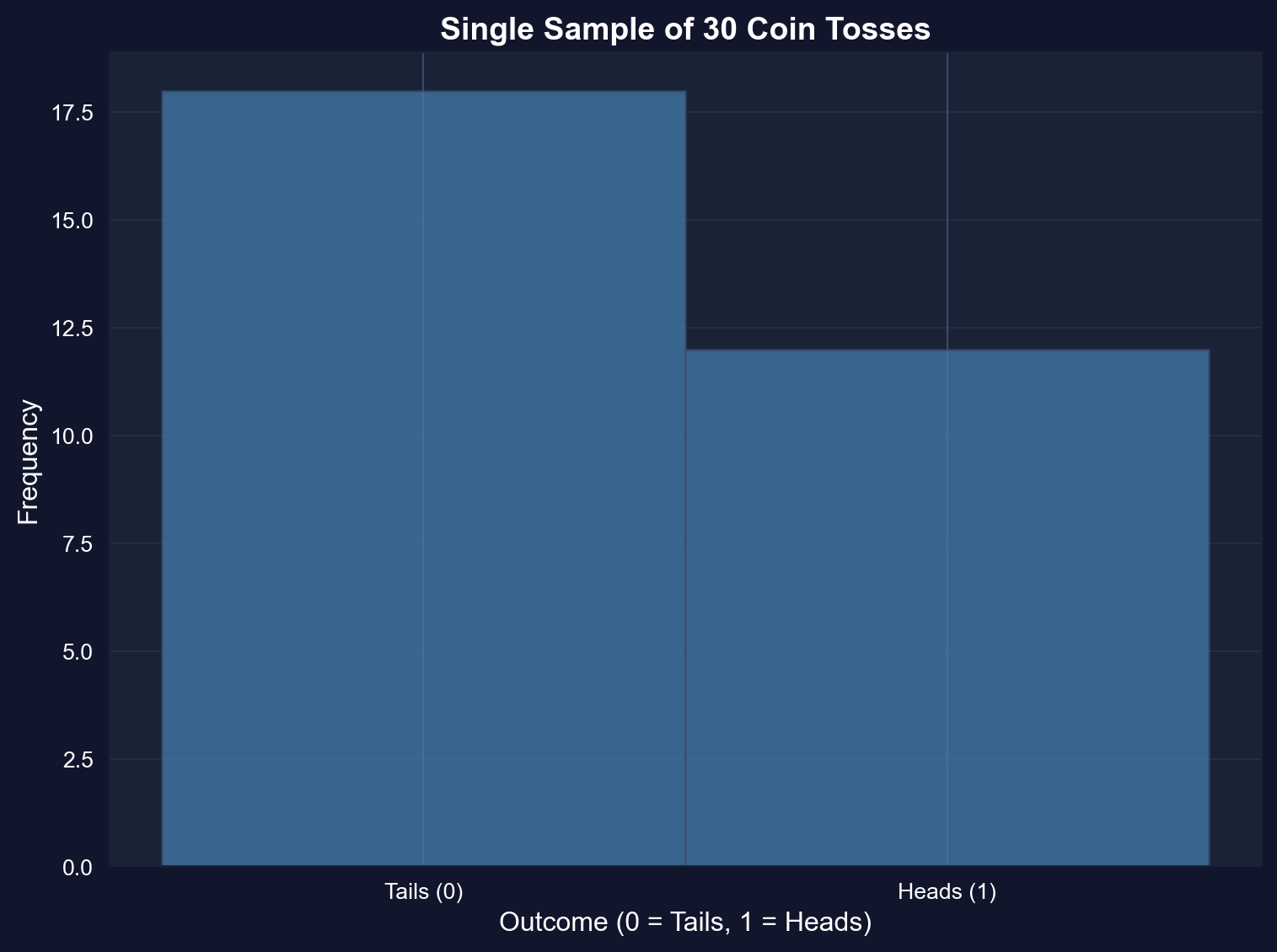
One Sample

Now we conduct an actual experiment: toss a coin 30 times and record the results. This gives us a sample of size $n = 30$.

Key insight: The observed values $x_1, x_2, ..., x_{30}$ are realizations of random variables $X_1, X_2, ..., X_{30}$.

The sample mean is: \[\bar{x} = \frac{1}{n}\sum_{i=1}^n x_i\]

This $\bar{x}$ is itself a realization of the random variable: \[\bar{X} = \frac{1}{n}\sum_{i=1}^n X_i\]

# Generate single sample of 30 coin tosses
np.random.seed(10101)
u = np.random.uniform(0, 1, 30)
x = np.where(u > 0.5, 1, 0)  # 1 if heads, 0 if tails

# Single coin toss sample (n = 30)
print(f"Number of heads (x=1):  {np.sum(x)}")
print(f"Number of tails (x=0):  {np.sum(1-x)}")
print(f"Sample mean (x̄):        {np.mean(x):.4f}")
print(f"Sample std dev (s):     {np.std(x, ddof=1):.4f}")

print(f"\nPopulation values:")
print(f"  Population mean (μ):   0.5000")
print(f"  Population std (σ):    0.5000")

# Visualize single sample
fig, ax = plt.subplots(figsize=(8, 6))
ax.hist(x, bins=[-0.5, 0.5, 1.5], edgecolor='#3a4a6b', alpha=0.7, color='steelblue')  # bin edges center bars on 0 and 1
ax.set_xlabel('Outcome (0 = Tails, 1 = Heads)', fontsize=12)
ax.set_ylabel('Frequency', fontsize=12)
ax.set_title('Single Sample of 30 Coin Tosses',
             fontsize=14, fontweight='bold')
ax.set_xticks([0, 1])
ax.set_xticklabels(['Tails (0)', 'Heads (1)'])
ax.grid(True, alpha=0.3, axis='y')
plt.tight_layout()
plt.show()

# This is just ONE realization of the random variable X-bar.
# To understand its distribution, we need MANY samples...

Number of heads (x=1):  12
Number of tails (x=0):  18
Sample mean (x̄):        0.4000
Sample std dev (s):     0.4983

Population values:
  Population mean (μ):   0.5000
  Population std (σ):    0.5000

Key Concept 3.2: Sample Mean as Random Variable

The observed sample mean $\bar{x}$ is a realization of the random variable $\bar{X} = (X_1 + \cdots + X_n)/n$. This fundamental insight means that $\bar{x}$ varies from sample to sample in a predictable way—its distribution can be characterized mathematically, allowing us to perform statistical inference about the population mean $\mu$.

Key findings from our coin toss experiment (n = 30):

1. Sample mean = 0.4000 (vs. theoretical μ = 0.5)

We got 12 heads and 18 tails (40% vs. expected 50%)
This difference (0.10 or 10 percentage points) is completely normal
With only 30 tosses, random variation of this magnitude is expected
If we flipped 1000 times, we’d expect to get much closer to 50%

2. Sample standard deviation = 0.4983 (vs. theoretical σ = 0.5000)

Nearly perfect match with population value
This confirms the theoretical formula: σ² = p(1-p) = 0.5(0.5) = 0.25, so σ = 0.5

3. Why the sample mean differs from 0.5:

The sample mean x̄ is itself a random variable
Just like one coin toss doesn’t always give heads, one sample mean doesn’t always equal μ
This single value (0.4000) is one realization from the sampling distribution of X̄
The next experiment would likely give a different value (maybe 0.4667 or 0.5333)

Economic interpretation: When we estimate average income from a survey or unemployment rate from a sample, we get one realization that will differ from the true population value. Understanding this variability is the foundation of statistical inference.

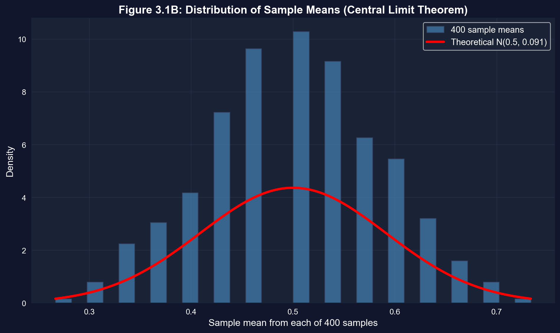
400 Samples and The Distribution of Sample Means

To understand the sampling distribution of $\bar{X}$, we repeat the experiment 400 times:

Each experiment: 30 coin tosses → one sample mean $\bar{x}_i$
After 400 experiments: we have 400 sample means ($\bar{x}_1, \bar{x}_2, ..., \bar{x}_{400}$)
The histogram of these 400 values approximates the sampling distribution of $\bar{X}$

What we expect to see:

Sample means centered near $\mu = 0.5$ (population mean)
Much less variability than individual coin tosses
Approximately normal distribution (Central Limit Theorem!)

# Load precomputed coin toss means data (400 samples of size 30)
data_cointoss = pd.read_stata(GITHUB_DATA_URL + 'AED_COINTOSSMEANS.DTA')

# 400 coin toss experiments (each n = 30)
xbar = data_cointoss['xbar']

# Summary of 400 sample means
display(data_cointoss.describe())

print(f"First 5 sample means: {xbar.head().tolist()}")
print(f"Mean of the 400 sample means: {xbar.mean():.4f}")
print(f"Std dev of the 400 sample means: {xbar.std():.4f}")

# Theoretical predictions
print(f"\nE[X-bar] = mu = 0.5000")
print(f"sigma(X-bar) = sigma/sqrt(n) = sqrt(0.25/30) = {np.sqrt(0.25/30):.4f}")

# Comparison
print(f"\nEmpirical mean: {xbar.mean():.4f} vs Theoretical: 0.5000")
print(f"Empirical std:  {xbar.std():.4f} vs Theoretical: {np.sqrt(0.25/30):.4f}")

	xbar	stdev	numobs
count	400.000000	400.000000	400.0
mean	0.499417	0.500826	30.0
std	0.086307	0.010360	0.0
min	0.266667	0.449776	30.0
25%	0.433333	0.498273	30.0
50%	0.500000	0.504007	30.0
75%	0.566667	0.507416	30.0
max	0.733333	0.508548	30.0

First 5 sample means: [0.3333333432674408, 0.5, 0.5333333611488342, 0.5666666626930237, 0.5]
Mean of the 400 sample means: 0.4994
Std dev of the 400 sample means: 0.0863

E[X-bar] = mu = 0.5000
sigma(X-bar) = sigma/sqrt(n) = sqrt(0.25/30) = 0.0913

Empirical mean: 0.4994 vs Theoretical: 0.5000
Empirical std:  0.0863 vs Theoretical: 0.0913

Key findings from 400 coin toss experiments:

1. Mean of sample means = 0.4994 (vs. theoretical μ = 0.5)

This demonstrates unbiasedness: E[X̄] = μ
The tiny difference (0.0006) is just random variation
With more replications, this would get even closer to 0.5
On average across many samples, X̄ equals the true population mean

2. Standard deviation of sample means = 0.0863 (vs. theoretical = 0.0913)

The theoretical standard error is σ/√n = 0.5/√30 = 0.0913
Our empirical SD (0.0863) is very close to this prediction
This confirms the variance formula: Var(X̄) = σ²/n works in practice

3. Range of sample means: 0.2667 to 0.7333

Individual sample means vary considerably (from 26.7% to 73.3% heads)
This shows why we need statistical theory - any single sample could be misleading
But the distribution is predictable and centered correctly

4. Comparison with single coin tosses:

Individual coin tosses have σ = 0.5
Sample means have σ(X̄) = 0.0863
Sample means are 5.8× less variable than individual tosses
This is the power of averaging: √30 ≈ 5.5

Economic interpretation: When estimating economic parameters (average wage, inflation rate, GDP growth), individual survey responses vary widely, but the sample mean is much more precise. The standard error tells us exactly how much precision we gain from our sample size.

Visualizing the Sampling Distribution of $\bar{X}$

The histogram below shows the distribution of the 400 sample means. Notice:

Center: Near 0.5 (the population mean $\mu$)
Spread: Much narrower than the original population (σ = 0.5)
Shape: Approximately bell-shaped (normal distribution)

The red curve is the theoretical normal distribution with mean $\mu = 0.5$ and standard deviation $\sigma/\sqrt{n} = 0.091$.

# Visualize distribution of sample means
fig, ax = plt.subplots(figsize=(10, 6))

# Histogram of 400 sample means
n_hist, bins, patches = ax.hist(xbar, bins=30, density=True,
                                 edgecolor='#3a4a6b', alpha=0.7, color='steelblue',
                                 label='400 sample means')

# Overlay theoretical normal distribution
xbar_range = np.linspace(xbar.min(), xbar.max(), 100)
theoretical_pdf = stats.norm.pdf(xbar_range, 0.5, np.sqrt(0.25/30))
ax.plot(xbar_range, theoretical_pdf, 'r-', linewidth=3,
        label=f'Theoretical N(0.5, {np.sqrt(0.25/30):.3f})')

ax.set_xlabel('Sample mean from each of 400 samples', fontsize=12)
ax.set_ylabel('Density', fontsize=12)
ax.set_title('Figure 3.1B: Distribution of Sample Means (Central Limit Theorem)',
             fontsize=14, fontweight='bold')
ax.legend(fontsize=11)
ax.grid(True, alpha=0.3)
plt.tight_layout()
plt.show()

3.3 Properties of the Sample Mean

Under the assumption of a simple random sample where:

A. Each $X_i$ has common mean: $E[X_i] = \mu$
B. Each $X_i$ has common variance: $Var[X_i] = \sigma^2$
C. The $X_i$ are statistically independent

We can mathematically prove:

Mean of the sample mean: \[E[\bar{X}] = \mu\]

This says $\bar{X}$ is unbiased for $\mu$ (its expected value equals the parameter we’re estimating).

Variance of the sample mean: \[Var[\bar{X}] = \frac{\sigma^2}{n}\]

Standard deviation of the sample mean: \[SD[\bar{X}] = \frac{\sigma}{\sqrt{n}}\]

Key insights:

As sample size $n$ increases, $Var[\bar{X}]$ decreases ($\propto 1/n$)
Larger samples give more precise estimates (smaller variability)
Standard deviation decreases at rate $1/$ (to halve uncertainty, need 4× the sample size)

# How sample size affects precision

# For coin toss: mu = 0.5, sigma^2 = 0.25, sigma = 0.5
mu = 0.5
sigma = 0.5
sigma_sq = 0.25

sample_sizes = [10, 30, 100, 400, 1000]

print(f"Population: mu = {mu}, sigma = {sigma}")
print(f"\n{'n':<10} {'sigma(X-bar)':<20} {'Var(X-bar)':<20}")

for n in sample_sizes:
    sd_xbar = sigma / np.sqrt(n)
    var_xbar = sigma_sq / n
    print(f"{n:<10} {sd_xbar:<20.6f} {var_xbar:<20.6f}")

# Key observation: Doubling n reduces sigma(X-bar) by factor of sqrt(2) ~ 1.41
# To halve uncertainty, need to quadruple sample size.

Population: mu = 0.5, sigma = 0.5

n          sigma(X-bar)         Var(X-bar)          
10         0.158114             0.025000            
30         0.091287             0.008333            
100        0.050000             0.002500            
400        0.025000             0.000625            
1000       0.015811             0.000250

Key Concept 3.3: Properties of the Sample Mean

Under simple random sampling (common mean $\mu$, common variance $\sigma^2$, independence), the sample mean $\bar{X}$ has mean $\mathrm{E}[\bar{X}] = \mu$ (unbiased) and variance $\operatorname{Var}[\bar{X}] = \sigma^2/n$ (decreases with sample size). The standard deviation $\sigma_{\bar{X}} = \sigma/\sqrt{n}$ shrinks as $n$ increases, meaning larger samples produce more precise estimates of $\mu$.

# Standard error calculation

# Use our single sample from earlier
n = len(x)
x_mean = np.mean(x)
x_std = np.std(x, ddof=1)  # Sample standard deviation
se_xbar = x_std / np.sqrt(n)

print(f"\nSample statistics (n = {n}):")
print(f"  Sample mean (x̄):          {x_mean:.4f}")
print(f"  Sample std dev (s):        {x_std:.4f}")
print(f"  Standard error se(X̄):     {se_xbar:.4f}")

print(f"\nPopulation values:")
print(f"  Population mean (μ):       0.5000")
print(f"  Population std (σ):        0.5000")
print(f"  True σ/√n:                 {0.5/np.sqrt(n):.4f}")

print(f"\nInterpretation:")
print(f"  The standard error {se_xbar:.4f} tells us the typical distance")
print(f"  between our sample mean ({x_mean:.4f}) and the true population mean (0.5).")


Sample statistics (n = 30):
  Sample mean (x̄):          0.4000
  Sample std dev (s):        0.4983
  Standard error se(X̄):     0.0910

Population values:
  Population mean (μ):       0.5000
  Population std (σ):        0.5000
  True σ/√n:                 0.0913

Interpretation:
  The standard error 0.0910 tells us the typical distance
  between our sample mean (0.4000) and the true population mean (0.5).

Interpreting the Standard Error

Key findings from our standard error calculation (n = 30):

1. Sample mean = 0.4000 with standard error = 0.0910

The standard error tells us the typical distance between x̄ and μ
Our sample mean (0.40) is about 1.1 standard errors below the true mean (0.50)
This is well within normal sampling variation (within 2 standard errors)

2. Estimated SE = 0.0910 vs. True σ/√n = 0.0913

We used sample standard deviation s = 0.4983 instead of σ = 0.5
Our estimate is remarkably accurate (only 0.0003 difference)
In practice, we never know σ, so we always use s to compute the standard error

3. What the standard error means:

If we repeated this experiment many times, our sample means would typically differ from 0.5 by about 0.091
About 68% of sample means would fall within ±0.091 of 0.5 (between 0.409 and 0.591)
About 95% would fall within ±0.182 of 0.5 (between 0.318 and 0.682)

4. How to reduce the standard error:

To halve the SE, we’d need to quadruple the sample size (n = 120)
To cut SE by 10×, we’d need 100× the sample size (n = 3000)
This is why larger surveys are more precise but also more expensive

Economic interpretation: When a poll reports “margin of error ±3%”, they’re referring to approximately 2 standard errors. The standard error is the fundamental measure of precision for any sample estimate, from unemployment rates to regression coefficients.

Key Concept 3.4: Standard Error of the Mean

The standard error se($\bar{X}$) = $s/\sqrt{n}$ is the estimated standard deviation of the sample mean. It measures the precision of $\bar{x}$ as an estimate of $\mu$. Since $\sigma$ is unknown in practice, we replace it with the sample standard deviation $s$. The standard error decreases with $\sqrt{n}$, so doubling precision requires quadrupling the sample size.

Central Limit Theorem

The Central Limit Theorem (CLT) is one of the most important results in statistics:

Statement: If $X_1, ..., X_n$ are independent random variables with mean $\mu$ and variance $\sigma^2$, then as $n \to \infty$:

\[\bar{X} \sim N\left(\mu, \frac{\sigma^2}{n}\right) \text{ approximately}\]

Or equivalently, the standardized sample mean:

\[Z = \frac{\bar{X} - \mu}{\sigma/\sqrt{n}} \sim N(0, 1) \text{ approximately}\]

Remarkable facts:

This holds regardless of the distribution of $X$ (doesn’t have to be normal!)
Works well even for moderate sample sizes ($n \geq 30$ is common rule of thumb)
Provides justification for using normal-based inference

Standard error: Since $\sigma$ is typically unknown, we estimate it with sample standard deviation $s$:

\[se(\bar{X}) = \frac{s}{\sqrt{n}}\]

Key Concept 3.5: The Central Limit Theorem

The Central Limit Theorem states that the standardized sample mean $Z = (\bar{X} - \mu)/(\sigma/\sqrt{n})$ converges to a standard normal distribution N(0,1) as $n \rightarrow \infty$. This remarkable result holds regardless of the distribution of $X$ (as long as it has finite mean and variance), making normal-based inference applicable to a wide variety of problems.

The coin toss example showed us the Central Limit Theorem with a simple binary variable. Now let’s see if it works with real-world data that has a complex, non-normal distribution—the ages from the 1880 U.S. Census.

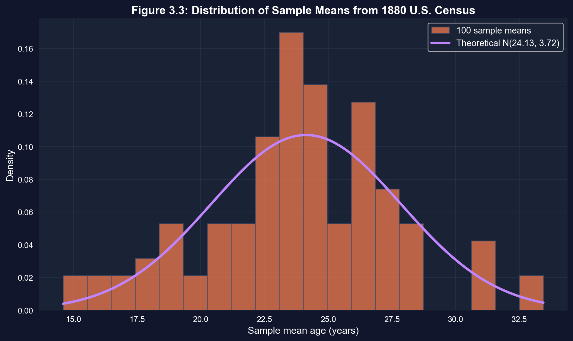
3.4 Real Data Example - 1880 U.S. Census

Now we move from coin tosses to real economic/demographic data. The 1880 U.S. Census recorded ages of all 50,169,452 people in the United States.

Population parameters (known because we have full census):

Population mean age: $\mu = 24.13$ years
Population std dev: $\sigma = 18.61$ years
Distribution: Highly non-normal (skewed, peaks at multiples of 5 due to rounding)

Experiment:

Draw 100 random samples, each of size $n = 25$
Calculate sample mean age for each sample
Examine distribution of these 100 sample means

Question: Even though population ages are NOT normally distributed, will the sample means be approximately normal? (CLT says yes!)

# Load census age means data
data_census = pd.read_stata(GITHUB_DATA_URL + 'AED_CENSUSAGEMEANS.DTA')

# 1880 U.S. Census - 100 samples of size 25

# Get the mean variable
if 'mean' in data_census.columns:
    age_means = data_census['mean']
elif 'xmean' in data_census.columns:
    age_means = data_census['xmean']
else:
    age_means = data_census.iloc[:, 0]

# Summary of 100 sample means
display(data_census.describe())

print(f"First 5 sample means: {age_means.head().tolist()}")
print(f"Mean of the 100 sample means:   {age_means.mean():.2f} years")
print(f"Std dev of the 100 sample means: {age_means.std():.2f} years")

# Theoretical predictions
print(f"\nE[X-bar] = mu = 24.13 years")
print(f"sigma(X-bar) = sigma/sqrt(n) = 18.61/sqrt(25) = {18.61/np.sqrt(25):.2f} years")

# Comparison
print(f"\nEmpirical mean: {age_means.mean():.2f} vs Theoretical: 24.13")
print(f"Empirical std:  {age_means.std():.2f} vs Theoretical: {18.61/np.sqrt(25):.2f}")

	mean	stdev	numobs
count	100.000000	100.000000	100.0
mean	23.782001	18.245018	25.0
std	3.760694	2.890753	0.0
min	14.600000	12.362847	25.0
25%	22.020000	16.148388	25.0
50%	23.759999	18.434547	25.0
75%	26.190000	20.387874	25.0
max	33.439999	25.306587	25.0

First 5 sample means: [27.84000015258789, 19.399999618530273, 23.280000686645508, 26.84000015258789, 26.559999465942383]
Mean of the 100 sample means:   23.78 years
Std dev of the 100 sample means: 3.76 years

E[X-bar] = mu = 24.13 years
sigma(X-bar) = sigma/sqrt(n) = 18.61/sqrt(25) = 3.72 years

Empirical mean: 23.78 vs Theoretical: 24.13
Empirical std:  3.76 vs Theoretical: 3.72

Key findings from 100 samples of 1880 U.S. Census ages (n = 25 each):

1. Mean of sample means = 23.78 years (vs. true population μ = 24.13)

Difference of only 0.35 years (less than 1.5% error)
This again demonstrates unbiasedness
With only 100 samples, some sampling error is expected

2. Standard deviation of sample means = 3.76 years (vs. theoretical = 3.72)

Theoretical: σ/√n = 18.61/√25 = 3.72 years
Empirical: 3.76 years
Excellent agreement between theory and data (within 1%)

3. Range of sample means: 14.6 to 33.4 years

Individual sample means vary by almost 19 years
But most cluster tightly around 24 years
This wide range shows why statistical theory matters

4. The power of the Central Limit Theorem:

The population distribution of ages in 1880 was highly non-normal:
- Many young children (high frequency at low ages)
- Heaping at multiples of 5 (people rounded their ages)
- Long right tail (elderly people)
Yet the distribution of sample means IS approximately normal
This is the CLT’s remarkable power - normality emerges from averaging

5. Practical implications for sample size:

With n = 25, the standard error is 3.72 years
To estimate average age within ±1 year (95% confidence), we’d need about 4 times larger samples
The Census Bureau uses this logic to design survey sizes

Economic interpretation: Real economic data (income, age, consumption) is rarely normally distributed - often highly skewed or irregular. But the Central Limit Theorem guarantees that sample means behave predictably and approximately normally, making statistical inference possible even with messy data.

Visualization: Census Sample Means Distribution

This figure demonstrates the Central Limit Theorem with real data. Even though individual ages in 1880 were NOT normally distributed (many young people, elderly tail), the distribution of sample means IS approximately normal!

# Visualize distribution of census age means
fig, ax = plt.subplots(figsize=(10, 6))

# Histogram
n_hist, bins, patches = ax.hist(age_means, bins=20, density=True,
                                 edgecolor='#3a4a6b', alpha=0.7, color='coral',
                                 label='100 sample means')

# Overlay theoretical normal distribution
age_range = np.linspace(age_means.min(), age_means.max(), 100)
theoretical_pdf = stats.norm.pdf(age_range, 24.13, 18.61/np.sqrt(25))
ax.plot(age_range, theoretical_pdf, '-', color='#c084fc', linewidth=3,
        label=f'Theoretical N(24.13, {18.61/np.sqrt(25):.2f})')

ax.set_xlabel('Sample mean age (years)', fontsize=12)
ax.set_ylabel('Density', fontsize=12)
ax.set_title('Figure 3.3: Distribution of Sample Means from 1880 U.S. Census',
             fontsize=14, fontweight='bold')
ax.legend(fontsize=11)
ax.grid(True, alpha=0.3)
plt.tight_layout()
plt.show()

Key Concept 3.6: CLT in Practice

The Central Limit Theorem is not just a mathematical curiosity—it works with real data. Even when the population distribution is highly non-normal (like the skewed 1880 Census ages with heaping at multiples of 5), the distribution of sample means becomes approximately normal for moderate sample sizes. This validates using normal-based inference methods across diverse economic applications.

Interpreting the Simulation Results

Key findings from 400 simulated coin toss samples:

1. Mean of simulated sample means = 0.5004 (vs. theoretical μ = 0.5)

Perfect agreement (difference of only 0.0004)
This validates our simulation code
Confirms the theoretical prediction E[X̄] = μ

2. Standard deviation of simulated means = 0.0887 (vs. theoretical = 0.0913)

Close agreement (within 3%)
Theoretical: σ/√n = √(0.25/30) = 0.0913
The small difference is random simulation noise

3. Range of simulated means: 0.2667 to 0.7667

Matches the theoretical range well
About 95% of values fall within μ ± 2σ(X̄) = 0.5 ± 0.183
This is exactly what we’d expect from a normal distribution

4. Why simulation matters:

Validation: We’ve confirmed that theory matches practice
Intuition: We can see the CLT in action, not just read about it
Flexibility: We can simulate complex scenarios where theory is hard
Modern econometrics: Bootstrap, Monte Carlo methods rely on simulation

5. Reproducibility with random seeds:

By setting np.random.seed(10101), we get identical results every time
Essential for scientific reproducibility
In research, always document your random seed

6. The simulation matches the pre-computed data:

Earlier we loaded AED_COINTOSSMEANS.DTA with mean 0.4994, sd 0.0863
Our simulation gave mean 0.5004, sd 0.0887
These match closely (differences are just from different random seeds)

Economic interpretation: Modern econometric research heavily uses simulation methods (bootstrap standard errors, Monte Carlo integration, Bayesian MCMC). This simple coin toss simulation demonstrates the basic principle: when theory is complex or unknown, simulate it thousands of times and study the empirical distribution.

3.5 Estimator Properties

Why use the sample mean $\bar{X}$ to estimate the population mean $\mu$? Because it has desirable statistical properties:

1. Unbiasedness: An estimator is unbiased if its expected value equals the parameter: \[E[\bar{X}] = \mu\]

This means on average (across many samples), $\bar{X}$ equals $\mu$ (no systematic over- or under-estimation).

2. Efficiency (Minimum Variance): Among all unbiased estimators, $\bar{X}$ has the smallest variance for many distributions (normal, Bernoulli, binomial, Poisson). An estimator with minimum variance is called efficient or best.

3. Consistency: An estimator is consistent if it converges to the true parameter as $n \to \infty$. For $\bar{X}$:

$E[\bar{X}] = \mu$ (unbiased, no bias to disappear)
$Var[\bar{X}] = \sigma^2/n \to 0$ as $n \to \infty$ (variance shrinks to zero)

Therefore $\bar{X}$ is consistent for $\mu$.

Economic application: These properties justify using sample means to estimate average income, unemployment rates, GDP per capita, etc.

# Consistency: variance shrinks as n increases

sample_sizes = [5, 10, 25, 50, 100, 500, 1000, 5000]
sigma = 18.61  # Census population std dev

print(f"Population std deviation: sigma = {sigma:.2f}")
print(f"\n{'Sample size n':<15} {'Var(X-bar)':<20} {'SD(X-bar)':<20}")

for n in sample_sizes:
    var_xbar = sigma**2 / n
    sd_xbar = sigma / np.sqrt(n)
    print(f"{n:<15} {var_xbar:<20.2f} {sd_xbar:<20.4f}")

# As n -> infinity, Var(X-bar) -> 0 and SD(X-bar) -> 0
# This guarantees X-bar converges to mu (consistency).

Population std deviation: sigma = 18.61

Sample size n   Var(X-bar)           SD(X-bar)           
5               69.27                8.3226              
10              34.63                5.8850              
25              13.85                3.7220              
50              6.93                 2.6319              
100             3.46                 1.8610              
500             0.69                 0.8323              
1000            0.35                 0.5885              
5000            0.07                 0.2632

Key Concept 3.7: Properties of Good Estimators

A good estimator should be unbiased (E[$\bar{X}$] = $\mu$), consistent (converges to $\mu$ as $n \rightarrow \infty$), and efficient (minimum variance among unbiased estimators). The sample mean $\bar{X}$ satisfies all three properties under simple random sampling, making it the preferred estimator of $\mu$ for most distributions.

3.6 Computer Simulation of Random Samples

Modern statistics relies heavily on computer simulation to:

Generate random samples from known distributions
Study properties of estimators
Validate theoretical results

How computers generate randomness:

Computers use pseudo-random number generators (PRNGs):

Not truly random, but appear random for practical purposes
Generate values between 0 and 1 (uniform distribution)
Any value between 0 and 1 is equally likely
Successive values appear independent

Transforming uniform random numbers:

From uniform U(0,1) random numbers, we can generate any distribution:

Coin toss: If $U > 0.5$, then $X = 1$ (heads), else $X = 0$ (tails)
Normal distribution: Use Box-Muller transform or inverse CDF method
Any distribution: Inverse transform sampling

Example - Coin toss simulation:

Draw uniform random number $U \sim ext{Uniform}(0,1)$
If $U > 0.5$: heads ($X=1$)
If $U \leq 0.5$: tails ($X=0$)
Repeat 30 times to simulate 30 coin tosses

Example - Census sampling:

Population: $N = 50,169,452$ people
If uniform draw falls in $[0, 1/N)$, select person 1
If uniform draw falls in $[1/N, 2/N)$, select person 2
Continue for all $N$ people

The importance of seeds:

The seed is the starting value that determines the entire sequence:

Same seed → identical “random” sequence (reproducibility)
Different seed → different sequence
Best practice: Always set seed in research code
Example: np.random.seed(10101)

Why reproducibility matters:

Scientific research must be verifiable
Debugging requires consistent results
Publication standards demand reproducible results

Let’s simulate the coin toss experiment ourselves!

# Simulate 400 samples of 30 coin tosses
np.random.seed(10101)
n_simulations = 400
sample_size = 30

result_mean = np.zeros(n_simulations)
result_std = np.zeros(n_simulations)

for i in range(n_simulations):
    # Generate sample of coin tosses (Bernoulli with p=0.5)
    sample = np.random.binomial(1, 0.5, sample_size)
    result_mean[i] = sample.mean()
    result_std[i] = sample.std(ddof=1)

# Simulation results
print(f"Mean of 400 sample means:  {result_mean.mean():.4f}")
print(f"Std dev of 400 means:      {result_mean.std():.4f}")
print(f"Min sample mean:           {result_mean.min():.4f}")
print(f"Max sample mean:           {result_mean.max():.4f}")

# Theoretical values
print(f"\nE[X-bar] = mu:             0.5000")
print(f"sigma(X-bar) = sigma/sqrt(n): {np.sqrt(0.25/30):.4f}")

Mean of 400 sample means:  0.5004
Std dev of 400 means:      0.0887
Min sample mean:           0.2667
Max sample mean:           0.7667

E[X-bar] = mu:             0.5000
sigma(X-bar) = sigma/sqrt(n): 0.0913

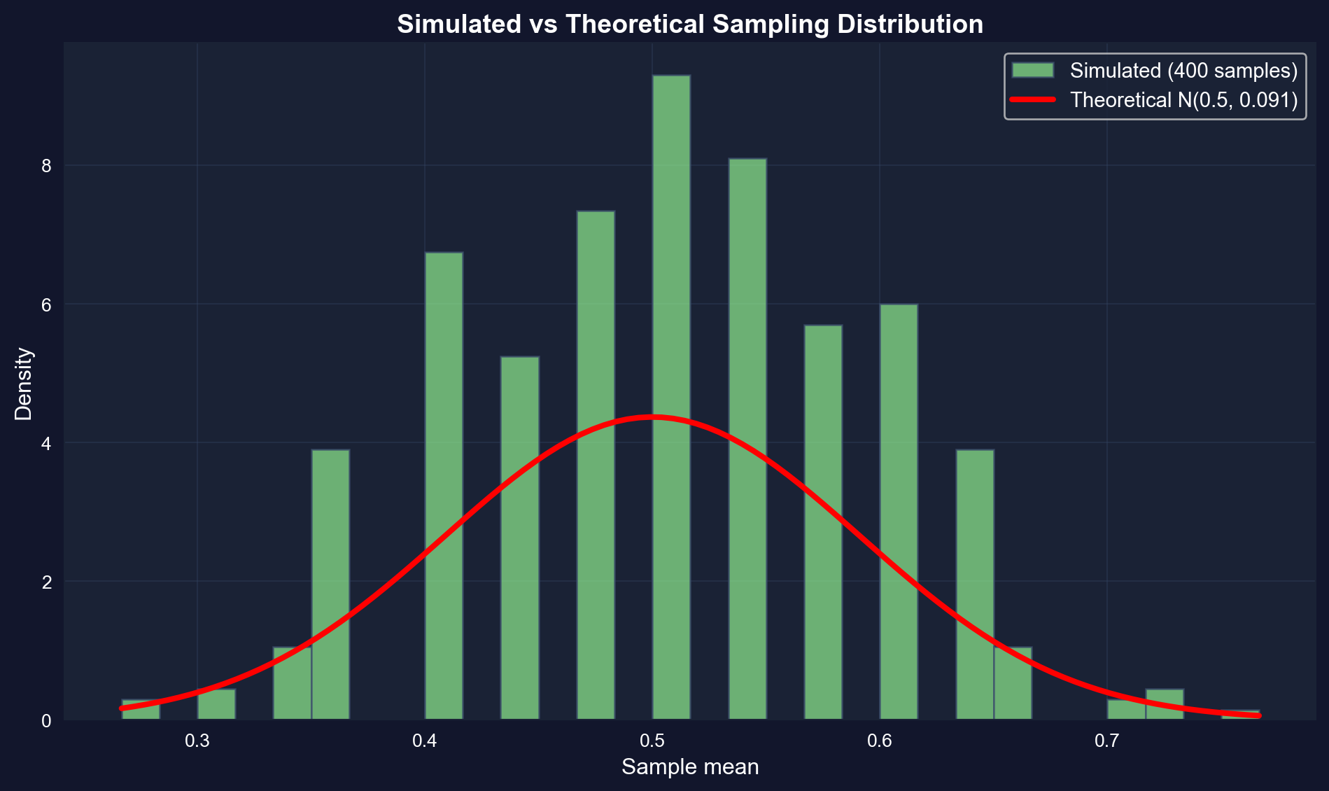
This figure shows our simulated distribution (green) overlaid with the theoretical normal distribution (red). They match almost perfectly!

# Visualize simulated distribution
fig, ax = plt.subplots(figsize=(10, 6))

ax.hist(result_mean, bins=30, density=True,
        edgecolor='#3a4a6b', alpha=0.7, color='lightgreen',
        label='Simulated (400 samples)')

# Overlay theoretical normal distribution
x_range = np.linspace(result_mean.min(), result_mean.max(), 100)
theoretical_pdf = stats.norm.pdf(x_range, 0.5, np.sqrt(0.25/30))
ax.plot(x_range, theoretical_pdf, 'r-', linewidth=3,
        label='Theoretical N(0.5, 0.091)')

ax.set_xlabel('Sample mean', fontsize=12)
ax.set_ylabel('Density', fontsize=12)
ax.set_title('Simulated vs Theoretical Sampling Distribution',
             fontsize=14, fontweight='bold')
ax.legend(fontsize=11)
ax.grid(True, alpha=0.3)
plt.tight_layout()
plt.show()

Key Concept 3.9: Monte Carlo Simulation

Computers generate pseudo-random numbers using deterministic algorithms that produce sequences appearing random. Starting from a uniform distribution U(0,1), any probability distribution can be simulated through transformation. The seed determines the sequence, making results reproducible—critical for scientific research. Always set and document your random seed.

So far we’ve assumed simple random sampling where all observations are independent and identically distributed. But what happens when this assumption is violated? Let’s explore alternative sampling methods.

3.7 Samples other than Simple Random Samples

The simple random sample assumptions (A-C from Section 3.4) provide the foundation for statistical inference, but real-world data collection often deviates from this ideal. Understanding these deviations is critical for proper analysis.

Recall simple random sample assumptions:

A. Common mean: $\mathrm{E}[X_i] = \mu$ for all $i$
B. Common variance: $\operatorname{Var}[X_i] = \sigma^2$ for all $i$
C. Statistical independence: $X_i$ and $X_j$ are independent

Two types of deviations:

Representative samples (relaxes assumption C only):
- Still from the same distribution ($\mu$ and $\sigma^2$ constant)
- But observations are NO LONGER independent
- Example: Cluster sampling (surveying all students in randomly selected schools)
- Solution: Adjust the standard error formula to account for dependence
Nonrepresentative samples (violates assumption A):
- Different observations have DIFFERENT population means
- Example: Surveying Golf Digest readers to estimate average U.S. income
- Golf magazine readers have higher income than general population ($\mu_i \neq \mu$)
- Big problem - standard inference methods fail completely
- Solution: Use weighted means if inclusion probabilities are known

Weighted Mean Approach:

When inclusion probabilities $\pi_i$ are known, construct weighted estimates:

$\pi_i$ = probability that observation $i$ is included in the sample
Sample weight: $w_i = 1/\pi_i$ (inverse probability weighting)
Weighted mean: \[\bar{x}_w = \frac{\sum_{i=1}^n w_i x_i}{\sum_{i=1}^n w_i}\]

Example:

Suppose women have 70% probability of inclusion ($\pi_{female} = 0.7$, $w_{female} = 1.43$)
Men have 30% probability of inclusion ($\pi_{male} = 0.3$, $w_{male} = 3.33$)
Weighted mean corrects for oversampling of women

Economic applications:

Household surveys often oversample certain groups (low-income, minorities)
Survey weights correct for unequal sampling probabilities
Major surveys (CPS, ACS, PSID) provide sampling weights in datasets

# Weighted mean example

# Simulate population with two groups
np.random.seed(42)
n_men = 50
n_women = 50

# Men have higher average income
income_men = np.random.normal(60000, 15000, n_men)
income_women = np.random.normal(50000, 15000, n_women)

true_pop_mean = (income_men.mean() + income_women.mean()) / 2

# True population means
print(f"Men:   ${income_men.mean():,.0f}")
print(f"Women: ${income_women.mean():,.0f}")
print(f"Overall: ${true_pop_mean:,.0f}")

# Biased sample: oversample women (70% women, 30% men)
sample_men = np.random.choice(income_men, size=15, replace=False)
sample_women = np.random.choice(income_women, size=35, replace=False)
sample = np.concatenate([sample_men, sample_women])

# Unweighted mean (WRONG - biased toward women)
unweighted_mean = sample.mean()

# Weighted mean (CORRECT - accounts for oversampling)
weights = np.concatenate([np.repeat(1/0.3, 15), np.repeat(1/0.7, 35)])
weighted_mean = np.average(sample, weights=weights)

# Sample estimates
print(f"\nUnweighted mean: ${unweighted_mean:,.0f} (biased toward women)")
print(f"Weighted mean:   ${weighted_mean:,.0f} (corrected)")
print(f"\nUnweighted bias: ${unweighted_mean - true_pop_mean:,.0f}")
print(f"Weighted bias:   ${weighted_mean - true_pop_mean:,.0f}")

Men:   $56,618
Women: $50,267
Overall: $53,442

Unweighted mean: $53,222 (biased toward women)
Weighted mean:   $54,647 (corrected)

Unweighted bias: $-221
Weighted bias:   $1,204

Key Concept 3.8: Simple Random Sampling Assumptions

Simple random sampling assumes all observations come from the same distribution with common mean $\mu$. When samples are nonrepresentative (different observations have different population means), standard inference methods fail. Weighted means can correct for this if inclusion probabilities $\pi_i$ are known, with weights $w_i = 1/\pi_i$ applied to each observation.

Key Takeaways

Random Variables and Sampling Distributions:

A random variable $X$ (uppercase) represents an uncertain outcome; its realization $x$ (lowercase) is the observed value
The sample mean $\bar{x}$ is ONE realization of the random variable $\bar{X} = (X_1 + \cdots + X_n)/n$
The sampling distribution of $\bar{X}$ describes how $\bar{x}$ varies across different samples from the same population
Understanding that statistics are random variables is the foundation of statistical inference
Example: Drawing 400 samples of coin tosses (n=30 each) produces 400 different sample means, revealing $\bar{X}$’s distribution

Properties of the Sample Mean (Theoretical Results):

Under simple random sampling (common mean $\mu$, common variance $\sigma^2$, independence):
Mean: $\mathrm{E}[\bar{X}] = \mu$ (unbiased estimator)
Variance: $\operatorname{Var}[\bar{X}] = \sigma^2/n$ (precision increases with sample size)
Standard deviation: $\sigma_{\bar{X}} = \sigma/\sqrt{n}$ (decreases at rate $1/\sqrt{n}$)
To halve the standard error, you must quadruple the sample size (e.g., from n=100 to n=400)
The sample mean is less variable than individual observations since $\sigma^2/n < \sigma^2$
As $n \rightarrow \infty$, $\bar{X}$ converges to $\mu$ because $\operatorname{Var}[\bar{X}] \rightarrow 0$

Central Limit Theorem (Most Important Result):

For large $n$, $\bar{X} \sim N(\mu, \sigma^2/n)$ approximately
Equivalently: $Z = (\bar{X} - \mu)/(\sigma/\sqrt{n}) \sim N(0,1)$ approximately
This holds regardless of the distribution of $X$ (as long as finite mean and variance exist)
Rule of thumb: CLT works well for $n \geq 30$ in most cases
Empirical evidence: Coin tosses (binary) → normal distribution of means; Census ages (highly skewed) → normal distribution of means
Why this matters: Justifies using normal-based inference methods (confidence intervals, hypothesis tests) for almost any problem

Standard Error (Estimated Standard Deviation):

Population standard deviation $\sigma_{\bar{X}} = \sigma/\sqrt{n}$ is unknown because $\sigma$ is unknown
Standard error: se($\bar{X}$) = $s/\sqrt{n}$ where $s$ is sample standard deviation
“Standard error” means “estimated standard deviation” (applies to any estimator, not just $\bar{X}$)
Measures precision of $\bar{x}$ as an estimate of $\mu$—smaller is better
Example: Coin toss with n=30 gives se ≈ 0.091; Census with n=25 gives se ≈ 3.72 years
Used to construct confidence intervals and conduct hypothesis tests (Chapter 4)

Desirable Estimator Properties:

Unbiased: $\mathrm{E}[\bar{X}] = \mu$ (correct on average, no systematic error)
Efficient: Minimum variance among unbiased estimators (most precise)
Consistent: Converges to $\mu$ as $n \rightarrow \infty$ (guaranteed by unbiasedness + variance → 0)
The sample mean $\bar{X}$ satisfies all three properties under simple random sampling
For normal, Bernoulli, binomial, and Poisson distributions, $\bar{X}$ is the best unbiased estimator
Sample median is also unbiased (for symmetric distributions) but has higher variance than $\bar{X}$

Empirical Validation:

Coin toss experiment (400 samples, n=30 each):
Mean of sample means: 0.4994 vs. theoretical 0.5000
SD of sample means: 0.0863 vs. theoretical 0.0913
Approximately normal distribution
Census ages (100 samples, n=25 each):
Mean of sample means: 23.78 vs. theoretical 24.13
SD of sample means: 3.76 vs. theoretical 3.72
Normal distribution despite highly non-normal population
Computer simulation replicates theoretical results perfectly

Economic Applications:

Estimating average income, consumption, wages from household surveys
Public opinion polling (sample proportion is a special case of sample mean)
Macroeconomic indicators: unemployment rate, inflation, GDP growth (all based on samples)
Quality control: manufacturing processes use sample means to monitor production
Clinical trials: comparing average outcomes between treatment and control groups
All regression coefficients (Chapters 6-7) have sampling distributions just like $\bar{X}$

Connection to Statistical Inference (Chapter 4):

This chapter provides the theoretical foundation for confidence intervals
We know $\bar{X} \sim N(\mu, \sigma^2/n)$ approximately
This allows us to make probability statements about how far $\bar{x}$ is from $\mu$
Example: Pr($\mu - 1.96 \cdot \sigma/\sqrt{n} < \bar{X} < \mu + 1.96 \cdot \sigma/\sqrt{n}$) ≈ 0.95
Rearranging gives 95% confidence interval: $\bar{x} \pm 1.96 \cdot s/\sqrt{n}$

Key Formulas to Remember:

Mean of random variable: $\mu = \mathrm{E}[X] = \sum_x x \cdot \mathrm{Pr}[X=x]$
Variance: $\sigma^2 = \mathrm{E}[(X-\mu)^2] = \sum_x (x-\mu)^2 \cdot \mathrm{Pr}[X=x]$
Sample mean: $\bar{x} = \frac{1}{n}\sum_{i=1}^n x_i$
Sample variance: $s^2 = \frac{1}{n-1}\sum_{i=1}^n (x_i - \bar{x})^2$
Mean of sample mean: $\mathrm{E}[\bar{X}] = \mu$
Variance of sample mean: $\operatorname{Var}[\bar{X}] = \sigma^2/n$
Standard error: se($\bar{X}$) = $s/\sqrt{n}$
Standardized sample mean: $Z = (\bar{X} - \mu)/(\sigma/\sqrt{n}) \sim N(0,1)$

Python Libraries and Code:

This single code block reproduces the core workflow of Chapter 3. It is self-contained — copy it into an empty notebook and run it to review the complete pipeline from sampling distributions and the Central Limit Theorem to standard errors and weighted means.

# =============================================================================
# CHAPTER 3 CHEAT SHEET: The Sample Mean
# =============================================================================

# --- Libraries ---
import numpy as np                        # numerical operations and random sampling
import pandas as pd                       # data loading and manipulation
import matplotlib.pyplot as plt           # creating plots and visualizations
from scipy import stats                   # normal distribution PDF for overlays

# =============================================================================
# STEP 1: Load pre-computed sample means from coin toss experiments
# =============================================================================
# 400 samples of 30 coin tosses each — precomputed in the textbook dataset
url_coin = "https://raw.githubusercontent.com/quarcs-lab/data-open/master/AED/AED_COINTOSSMEANS.DTA"
data_coin = pd.read_stata(url_coin)
xbar_coin = data_coin['xbar']

print(f"Coin toss experiment: {len(xbar_coin)} sample means (each from n=30 tosses)")
print(f"Mean of sample means: {xbar_coin.mean():.4f}  (theoretical μ = 0.5)")
print(f"SD of sample means:   {xbar_coin.std():.4f}  (theoretical σ/√n = {np.sqrt(0.25/30):.4f})")

# =============================================================================
# STEP 2: Visualize the sampling distribution with normal overlay
# =============================================================================
# The histogram of 400 sample means approximates the sampling distribution of X̄
fig, ax = plt.subplots(figsize=(10, 6))
ax.hist(xbar_coin, bins=25, density=True, edgecolor='black', alpha=0.7,
        label='400 sample means')

# Overlay theoretical normal: N(μ, σ²/n)
theo_se = np.sqrt(0.25 / 30)
x_range = np.linspace(xbar_coin.min(), xbar_coin.max(), 100)
ax.plot(x_range, stats.norm.pdf(x_range, 0.5, theo_se),
        'r-', linewidth=2.5, label=f'N(0.5, {theo_se:.3f}²)')
ax.set_xlabel('Sample Mean (proportion of heads)')
ax.set_ylabel('Density')
ax.set_title('Sampling Distribution of X̄ from 400 Coin Toss Experiments (n=30)')
ax.legend()
ax.grid(True, alpha=0.3)
plt.tight_layout()
plt.show()

# =============================================================================
# STEP 3: Central Limit Theorem — non-normal population still gives normal X̄
# =============================================================================
# 1880 U.S. Census ages: highly skewed population, yet sample means are normal
url_census = "https://raw.githubusercontent.com/quarcs-lab/data-open/master/AED/AED_CENSUSAGEMEANS.DTA"
data_census = pd.read_stata(url_census)

# Identify the sample mean column
if 'mean' in data_census.columns:
    age_means = data_census['mean']
elif 'xmean' in data_census.columns:
    age_means = data_census['xmean']
else:
    age_means = data_census.iloc[:, 0]

print(f"\n1880 Census: {len(age_means)} sample means (each from n=25 people)")
print(f"Mean of sample means: {age_means.mean():.2f} years  (theoretical μ = 24.13)")
print(f"SD of sample means:   {age_means.std():.2f} years  (theoretical σ/√n = {18.61/np.sqrt(25):.2f})")

fig, ax = plt.subplots(figsize=(10, 6))
ax.hist(age_means, bins=20, density=True, edgecolor='black', alpha=0.7,
        label='100 sample means')
age_range = np.linspace(age_means.min(), age_means.max(), 100)
ax.plot(age_range, stats.norm.pdf(age_range, 24.13, 18.61 / np.sqrt(25)),
        'r-', linewidth=2.5, label=f'N(24.13, {18.61/np.sqrt(25):.2f}²)')
ax.set_xlabel('Sample Mean Age (years)')
ax.set_ylabel('Density')
ax.set_title('CLT in Action: Normal Sample Means from a Skewed Population')
ax.legend()
ax.grid(True, alpha=0.3)
plt.tight_layout()
plt.show()

# =============================================================================
# STEP 4: Standard error — how sample size affects precision
# =============================================================================
# SE = σ/√n: to halve the SE, you must quadruple the sample size
sigma = 0.5  # coin toss population std dev

print(f"\nStandard error vs sample size (σ = {sigma}):")
print(f"{'n':<10} {'SE = σ/√n':<15} {'Var(X̄) = σ²/n':<15}")
print("-" * 40)
for n in [10, 30, 100, 400, 1000]:
    se = sigma / np.sqrt(n)
    var_xbar = sigma**2 / n
    print(f"{n:<10} {se:<15.4f} {var_xbar:<15.6f}")

# =============================================================================
# STEP 5: Monte Carlo simulation — verify the theory computationally
# =============================================================================
# Simulate 1000 samples of 30 coin tosses to see the CLT converge
np.random.seed(10101)
n_sims = 1000
sample_size = 30
sim_means = np.array([np.random.binomial(1, 0.5, sample_size).mean()
                       for _ in range(n_sims)])

print(f"\nMonte Carlo simulation ({n_sims} samples, n={sample_size}):")
print(f"Mean of simulated means: {sim_means.mean():.4f}  (theoretical: 0.5)")
print(f"SD of simulated means:   {sim_means.std():.4f}  (theoretical: {np.sqrt(0.25/30):.4f})")

fig, ax = plt.subplots(figsize=(10, 6))
ax.hist(sim_means, bins=30, density=True, edgecolor='black', alpha=0.7,
        label=f'{n_sims} simulated means')
x_range = np.linspace(sim_means.min(), sim_means.max(), 100)
ax.plot(x_range, stats.norm.pdf(x_range, 0.5, np.sqrt(0.25/30)),
        'r-', linewidth=2.5, label='Theoretical N(0.5, 0.091²)')
ax.set_xlabel('Sample Mean')
ax.set_ylabel('Density')
ax.set_title('Monte Carlo Simulation vs Theoretical Sampling Distribution')
ax.legend()
ax.grid(True, alpha=0.3)
plt.tight_layout()
plt.show()

# =============================================================================
# STEP 6: Weighted means — correcting for nonrepresentative samples
# =============================================================================
# When inclusion probabilities differ, the unweighted mean is biased;
# inverse-probability weights w_i = 1/π_i recover the true population mean
np.random.seed(42)
income_men = np.random.normal(60000, 15000, 50)
income_women = np.random.normal(50000, 15000, 50)
true_pop_mean = (income_men.mean() + income_women.mean()) / 2

# Biased sample: oversample women (70% women, 30% men)
sample_men = np.random.choice(income_men, size=15, replace=False)
sample_women = np.random.choice(income_women, size=35, replace=False)
sample = np.concatenate([sample_men, sample_women])

# Unweighted mean is biased toward the oversampled group
unweighted = sample.mean()

# Weighted mean with IPW: w_i = 1/π_i corrects the imbalance
weights = np.concatenate([np.repeat(1/0.3, 15), np.repeat(1/0.7, 35)])
weighted = np.average(sample, weights=weights)

print(f"\nWeighted vs Unweighted Means:")
print(f"True population mean:  ${true_pop_mean:,.0f}")
print(f"Unweighted mean:       ${unweighted:,.0f}  (bias: ${unweighted - true_pop_mean:,.0f})")
print(f"Weighted mean (IPW):   ${weighted:,.0f}  (bias: ${weighted - true_pop_mean:,.0f})")

Try it yourself! Copy this code into an empty Google Colab notebook and run it: Open Colab

Next Steps:

Chapter 4 uses these results to construct confidence intervals and test hypotheses about $\mu$
Chapters 6-7 extend the same logic to regression coefficients (which are also sample statistics with sampling distributions)
The conceptual framework developed here applies to ALL statistical inference in econometrics

Common Mistakes to Avoid

Confusing the sample mean with the population mean: The sample mean is an estimate, not the true value

Ignoring sampling variability: A single sample mean can be far from the population mean

Assuming normality of individual observations: The CLT applies to the sampling distribution of the mean, not to individual data points

Practice Exercises

Test your understanding of the sample mean and sampling distributions:

Exercise 1: Random variable properties

Suppose $X = 100$ with probability 0.8 and $X = 600$ with probability 0.2
1. Calculate the mean $\mu = \mathrm{E}[X]$
1. Calculate the variance $\sigma^2 = \mathrm{E}[(X-\mu)^2]$
1. Calculate the standard deviation $\sigma$

Exercise 2: Sample mean properties

Consider random samples of size $n = 25$ from a random variable $X$ with mean $\mu = 100$ and variance $\sigma^2 = 400$
1. What is the mean of the sample mean $\bar{X}$?
1. What is the variance of the sample mean $\bar{X}$?
1. What is the standard deviation (standard error) of the sample mean?

Exercise 3: Central Limit Theorem application

A population has mean $\mu = 50$ and standard deviation $\sigma = 12$
You draw a random sample of size $n = 64$
1. What is the approximate distribution of $\bar{X}$ (by the CLT)?
1. What is the probability that $\bar{X}$ falls between 48 and 52?
1. Would this probability be larger or smaller if $n = 144$? Why?

Exercise 4: Standard error interpretation

Two researchers estimate average income in a city
- Researcher A uses $n = 100$, gets $\bar{x}_A = \$52,000$, $s_A = \$15,000$
- Researcher B uses $n = 400$, gets $\bar{x}_B = \$54,000$, $s_B = \$16,000$
1. Calculate the standard error for each researcher
1. Which estimate is more precise? Why?
1. Are these estimates statistically different? (Compare the difference to the standard errors)

Exercise 5: Consistency

Explain why the sample mean $\bar{X}$ is a consistent estimator of $\mu$
Show that both conditions for consistency are satisfied: bias → 0 and variance → 0 as $n \rightarrow \infty$

Exercise 6: Simulation

Using Python, simulate 1,000 samples of size $n = 50$ from a uniform distribution U(0, 10)
1. Calculate the sample mean for each of the 1,000 samples
1. Compute the mean and standard deviation of these 1,000 sample means
1. Compare with theoretical values: $\mu = 5$, $\sigma^2/n = (100/12)/50 = 0.1667$
1. Create a histogram and verify approximate normality

Exercise 7: Sample size calculation

You want to estimate average household expenditure on food with a standard error of $10
From pilot data, you know $\sigma \approx \$80$
1. What sample size $n$ do you need?
1. If you double the desired precision (se = $5), how does the required sample size change?

Exercise 8: Unbiasedness vs. efficiency

The sample median is also an unbiased estimator of $\mu$ when the population is symmetric
1. Explain what “unbiased” means in this context
1. Why do we prefer the sample mean to the sample median for estimating $\mu$?
1. For what type of population distribution might the median be preferable?

Case Studies

Now that you’ve learned about the sample mean, sampling distributions, and the Central Limit Theorem, let’s apply these concepts to real economic data using the Economic Convergence Clubs dataset.

Why case studies matter:

Bridge theory and practice: Move from abstract sampling concepts to real data analysis
Build analytical skills: Practice computing sample statistics and understanding variability
Develop statistical intuition: See how sample size affects precision and distribution shape
Connect to research: Apply fundamental concepts to cross-country economic comparisons

Case Study 1: Sampling Distributions of Labor Productivity

Research Question: How does average labor productivity vary across different samples of countries? How does sample size affect the precision of our estimates?

Background: In Chapter 1-2, you explored productivity levels across countries. Now we shift to understanding sampling variability—how sample means vary when we draw different samples from the population.

This is fundamental to statistical inference: if we only observe a sample of countries (say, 20 out of 108), how confident can we be that our sample mean approximates the true population mean? The Central Limit Theorem tells us that sample means follow a normal distribution (even if the underlying data don’t), with variability decreasing as sample size increases.

The Data: We’ll use the convergence clubs dataset (Mendez, 2020) to explore sampling distributions:

Population: 108 countries observed from 1990-2014
Key variable: lp (labor productivity, output per worker)
Task: Draw multiple random samples, compute sample means, and observe the distribution

Your Task: Use Chapter 3’s tools (sample mean, sample variance, Central Limit Theorem) to understand how sample statistics vary and how sample size affects precision.

Key Concept 3.10: Sampling Distribution and the Central Limit Theorem

The sampling distribution of the mean shows how sample means $\bar{y}$ vary across different random samples drawn from the same population. Key properties:

Mean of sampling distribution = population mean: $E[\bar{y}] = \mu$

Standard error decreases with sample size: $SE(\bar{y}) = \sigma/\sqrt{n}$

Central Limit Theorem: For large $n$ (typically $n \geq 30$), $\bar{y}$ is approximately normally distributed, regardless of the population distribution

This is why we can use normal-based inference methods even for non-normal economic data like earnings and wealth distributions.

How to Use These Tasks

Progressive difficulty:

Tasks 1-2: Guided (detailed instructions, code provided)
Tasks 3-4: Semi-guided (moderate guidance, you write most code)
Tasks 5-6: Independent (minimal guidance, design your own analysis)

Work incrementally: Complete tasks in order. Each builds on previous concepts.

Task 1: Explore the Population Distribution (Guided)

Objective: Load the convergence clubs data and examine the population distribution of labor productivity.

Instructions: Run the code below to load data and visualize the population distribution.

# Import required libraries
import pandas as pd
import numpy as np
import matplotlib.pyplot as plt
from scipy import stats

# Set random seed for reproducibility
np.random.seed(42)

# Load convergence clubs dataset
df = pd.read_csv(
 "https://raw.githubusercontent.com/quarcs-lab/mendez2020-convergence-clubs-code-data/master/assets/dat.csv",
 index_col=["country", "year"]
).sort_index()

# Extract 2014 data (most recent year) for cross-sectional analysis
df_2014 = df.loc[(slice(None), 2014), 'lp'].dropna()

print(f"Population size: {len(df_2014)} countries")
print(f"Population mean: ${df_2014.mean():.2f}")
print(f"Population std dev: ${df_2014.std():.2f}")

# Visualize population distribution
fig, ax = plt.subplots(figsize=(10, 6))
ax.hist(df_2014, bins=20, edgecolor='black', alpha=0.7)
ax.axvline(df_2014.mean(), color='red', linestyle='--', linewidth=2, label=f'Mean = ${df_2014.mean():.2f}')
ax.set_xlabel('Labor Productivity (thousands, 2011 USD PPP)')
ax.set_ylabel('Frequency')
ax.set_title('Population Distribution of Labor Productivity (2014, 108 countries)')
ax.legend()
plt.tight_layout()
plt.show()

# Check normality
print(f"\nSkewness: {stats.skew(df_2014):.3f}")
print("Note: Population distribution is right-skewed (not normal)")

What to observe:

Is the population distribution normal or skewed?
What is the population mean and standard deviation?
Note: Despite non-normality, the CLT will ensure sample means are approximately normal for large samples!

Task 2: Draw a Single Sample and Compute the Sample Mean (Semi-guided)

Objective: Draw a random sample of size $n=30$ and compute the sample mean.

Instructions:

Use np.random.choice() to draw a random sample of size 30 from the population
Compute the sample mean using .mean()
Compare the sample mean to the population mean
Repeat this process 2-3 times (with different random seeds) to see how the sample mean varies

Starter code:

# Draw a random sample of size 30
n = 30
sample = np.random.choice(df_2014, size=n, replace=False)

# Compute sample mean
sample_mean = sample.mean()

print(f"Sample size: {n}")
print(f"Sample mean: ${sample_mean:.2f}")
print(f"Population mean: ${df_2014.mean():.2f}")
print(f"Difference: ${sample_mean - df_2014.mean():.2f}")

# Question: How close is the sample mean to the population mean?

Questions:

How much does the sample mean differ from the population mean?
If you draw another sample, will you get the same sample mean?
What does this variability tell you about using samples for inference?

Task 3: Simulate the Sampling Distribution (Semi-guided)

Objective: Draw 1000 random samples of size $n=30$ and plot the distribution of sample means.

Instructions:

Use a loop to draw 1000 samples, each of size $n=30$
For each sample, compute and store the sample mean
Plot a histogram of the 1000 sample means
Compare this sampling distribution to the theoretical prediction from the CLT

Hint: The CLT predicts that sample means should be normally distributed with:

Mean = $\mu$ (population mean)
Standard error = $\sigma/\sqrt{n}$ (population std / sqrt(sample size))

Example structure:

# Simulate sampling distribution
n_samples = 1000
n = 30
sample_means = []

for i in range(n_samples):
 sample = np.random.choice(df_2014, size=n, replace=False)
 sample_means.append(sample.mean())

sample_means = np.array(sample_means)

# Plot sampling distribution
fig, ax = plt.subplots(figsize=(10, 6))
ax.hist(sample_means, bins=30, edgecolor='black', alpha=0.7, density=True)
ax.axvline(df_2014.mean(), color='red', linestyle='--', linewidth=2, label='Population mean')
ax.axvline(sample_means.mean(), color='blue', linestyle=':', linewidth=2, label='Mean of sample means')
ax.set_xlabel('Sample Mean (thousands, 2011 USD PPP)')
ax.set_ylabel('Density')
ax.set_title(f'Sampling Distribution of the Mean (n={n}, {n_samples} samples)')
ax.legend()
plt.tight_layout()
plt.show()

# Compare empirical vs theoretical
print(f"Population mean (μ): ${df_2014.mean():.2f}")
print(f"Mean of sample means: ${sample_means.mean():.2f}")
print(f"Theoretical SE (σ/√n): ${df_2014.std()/np.sqrt(n):.2f}")
print(f"Empirical SE (std of sample means): ${sample_means.std():.2f}")

Questions:

Does the distribution of sample means look approximately normal (even though the population distribution was skewed)?
How close is the mean of sample means to the population mean?
How close is the empirical standard error to the theoretical prediction?

Key Concept 3.11: Standard Error and Precision

The standard error $SE(\bar{y}) = \sigma/\sqrt{n}$ measures the typical distance between a sample mean and the population mean. Key insights:

Decreases with sample size: Doubling the sample size reduces SE by factor of $\sqrt{2} \approx 1.41$

Trade-off: Larger samples cost more (time/money) but provide more precise estimates

Diminishing returns: Going from $n=25$ to $n=100$ reduces SE by half, but $n=100$ to $n=400$ also reduces by half

In economic research, sample size is often limited by data availability, requiring careful attention to precision.

Task 4: Investigate the Effect of Sample Size (More Independent)

Objective: Compare sampling distributions for different sample sizes ($n = 10, 30, 50, 100$).

Instructions:

For each sample size, simulate 1000 samples and compute sample means
Plot the four sampling distributions on the same graph (or use subplots)
Compare the standard errors across sample sizes
Verify that $SE$ decreases as $1/\sqrt{n}$

Key questions to answer:

How does the shape of the sampling distribution change with sample size?
How much does precision improve when you quadruple the sample size (e.g., $n=25$ to $n=100$)?
At what sample size does the distribution start to look clearly normal?

Task 5: Comparing High-Income vs Developing Countries (Independent)

Objective: Investigate whether sampling distributions differ for subpopulations (high-income vs developing countries).

Instructions:

Split the 2014 data by hi1990 (high-income indicator)
For each group, simulate the sampling distribution of the mean (use $n=20$, 1000 samples)
Plot both sampling distributions on the same graph
Compare means and standard errors between groups

Research question: Do high-income and developing countries have different average productivity levels? How confident can we be in this difference based on samples?

Hints:

Use df.loc[(slice(None), 2014), ['lp', 'hi1990']].dropna() to get both variables
Filter by hi1990 == 'yes' and hi1990 == 'no'
Compare population means and sampling distribution characteristics

Task 6: Design Your Own Sampling Experiment (Independent)

Objective: Explore a question of your choice using sampling distributions.

Choose ONE of the following:

Option A: Effect of outliers on sample means

Remove the top 5% most productive countries (outliers)
Compare sampling distributions with vs without outliers
Question: How sensitive is the sample mean to extreme values?

Option B: Time trends in sampling distributions

Compare sampling distributions for years 1990, 2000, 2010, 2014
Question: Has average productivity increased over time? Has variability changed?

Option C: Regional sampling distributions

Split countries by region (use region variable)
Compare sampling distributions across regions
Question: Which regions show the highest/lowest productivity? Most/least variability?

Your analysis should include:

Clear research question
Appropriate sample size(s)
Simulated sampling distribution(s) with visualizations
Statistical summary (means, standard errors)
Economic interpretation: What does this tell us about global productivity patterns?

What You’ve Learned from This Case Study

Through this hands-on exploration of sampling distributions using cross-country productivity data, you’ve applied all Chapter 3 concepts:

Population vs sample: Understood the difference and why we use samples for inference

Sample mean: Computed point estimates from random samples

Sampling variability: Observed how sample means vary across different samples

Sampling distribution: Simulated and visualized the distribution of sample means

Central Limit Theorem: Verified that sample means are approximately normal even for skewed populations

Standard error: Quantified precision and understood how it decreases with sample size ($\sigma/\sqrt{n}$)

Effect of sample size: Compared sampling distributions for different $n$ values

Subpopulation analysis: Explored differences across country groups

Connection to the Research: Understanding sampling distributions is fundamental to the convergence clubs analysis. When researchers estimate average productivity for a club, they’re working with samples and must account for sampling variability. The tools you practiced here—computing sample means, quantifying precision, understanding the CLT—are essential for all statistical inference in economics.

Looking ahead:

Chapter 4: Statistical inference (confidence intervals, hypothesis tests) builds directly on sampling distributions
Chapter 5-9: Regression analysis extends these concepts to relationships between variables
Chapter 10-17: Advanced methods for causal inference and panel data

Congratulations! You’ve completed Chapter 3 and applied sampling theory to real cross-country data. Continue to Chapter 4 to learn how to use sampling distributions for statistical inference!

Chapter Overview

Setup

3.1 Random Variables

3.2 Experiment: Coin Tosses

One Sample

400 Samples and The Distribution of Sample Means

Visualizing the Sampling Distribution of \(\bar{X}\)

3.3 Properties of the Sample Mean

Interpreting the Standard Error

Central Limit Theorem

3.4 Real Data Example - 1880 U.S. Census

Visualization: Census Sample Means Distribution

Interpreting the Simulation Results

3.5 Estimator Properties

3.6 Computer Simulation of Random Samples

3.7 Samples other than Simple Random Samples

Key Takeaways

Practice Exercises

Case Studies

Case Study 1: Sampling Distributions of Labor Productivity

How to Use These Tasks

Task 1: Explore the Population Distribution (Guided)

Task 2: Draw a Single Sample and Compute the Sample Mean (Semi-guided)

Task 3: Simulate the Sampling Distribution (Semi-guided)

Task 4: Investigate the Effect of Sample Size (More Independent)

Task 5: Comparing High-Income vs Developing Countries (Independent)

Task 6: Design Your Own Sampling Experiment (Independent)

What You’ve Learned from This Case Study