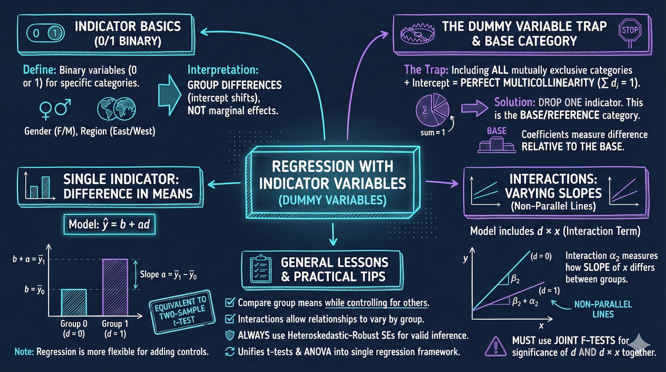
14. Regression with Indicator Variables

metricsAI: An Introduction to Econometrics with Python and AI in the Cloud

This notebook provides an interactive introduction to regression with indicator variables (also called dummy variables or categorical variables). All code runs directly in Google Colab without any local setup.

🎬 AI Video ✨ AI Slides 📊 Cameron Slides ✏️ Quiz 🤖 AI Tutor

Chapter Overview

This chapter focuses on regression analysis when some regressors are indicator variables. Indicator variables are binary (0/1) variables that record whether an observation falls into a particular category.

What You’ll Learn

By the end of this chapter, you will be able to:

Understand indicator (dummy) variables and their role in regression analysis
Interpret regression coefficients when regressors are categorical variables
Use indicator variables to compare group means and test for differences
Understand the relationship between regression on indicators and t-tests/ANOVA
Incorporate indicator variables alongside continuous regressors to control for categories
Create and interpret interaction terms between indicators and continuous variables
Apply the dummy variable trap rule when using sets of mutually exclusive indicators
Choose appropriate base categories and interpret coefficients relative to the base
Conduct joint F-tests for the significance of sets of indicator variables
Apply indicator variable techniques to real earnings data

Chapter Outline

14.1 Indicator Variables: Single Binary Variable
14.2 Indicator Variable with Additional Regressors
14.3 Interactions with Indicator Variables
14.4 Testing for Structural Change
14.5 Sets of Indicator Variables
Key Takeaways – Chapter review and consolidated lessons
Practice Exercises – Reinforce your understanding
Case Studies – Apply indicator variables to cross-country data

Dataset used:

AED_EARNINGS_COMPLETE.DTA: 872 full-time workers aged 25-65 in 2000

Key economic questions:

Is there a gender earnings gap? How large is it after controlling for education and experience?
How do the returns to education differ by gender?
Do earnings differ across types of workers (self-employed, private, government)?
Can we test for structural differences between groups?

Setup

First, we import the necessary Python packages and configure the environment for reproducibility. All data will stream directly from GitHub.

Setup: Import libraries and configure environment

# Import required packages
import numpy as np
import pandas as pd
import matplotlib.pyplot as plt
import seaborn as sns
import statsmodels.api as sm
from statsmodels.formula.api import ols
from scipy import stats
from scipy.stats import f_oneway
from statsmodels.stats.anova import anova_lm
import random
import os

# Set random seeds for reproducibility
RANDOM_SEED = 42
random.seed(RANDOM_SEED)
np.random.seed(RANDOM_SEED)
os.environ['PYTHONHASHSEED'] = str(RANDOM_SEED)

# GitHub data URL
GITHUB_DATA_URL = "https://raw.githubusercontent.com/quarcs-lab/data-open/master/AED/"

# Set plotting style (dark theme matching book design)
plt.style.use('dark_background')
sns.set_style("darkgrid")
plt.rcParams.update({
    'axes.facecolor': '#1a2235',
    'figure.facecolor': '#12162c',
    'grid.color': '#3a4a6b',
    'figure.figsize': (10, 6),
    'text.color': 'white',
    'axes.labelcolor': 'white',
    'xtick.color': 'white',
    'ytick.color': 'white',
    'axes.edgecolor': '#1a2235',
})

# Chapter 14: Regression With Indicator Variables
# Setup complete! Ready to explore regression with indicator variables.

Data Preparation

We’ll work with the earnings dataset which contains information on 872 full-time workers.

Key variables:

earnings: Annual earnings in dollars
gender: 1=female, 0=male
education: Years of schooling
age: Age in years
hours: Usual hours worked per week
dself: 1=self-employed, 0=not
dprivate: 1=private sector employee, 0=not
dgovt: 1=government sector employee, 0=not
genderbyeduc: Gender × Education interaction
genderbyage: Gender × Age interaction
genderbyhours: Gender × Hours interaction

# Load earnings data
data = pd.read_stata(GITHUB_DATA_URL + 'AED_EARNINGS_COMPLETE.DTA')

print("Data structure:")
print(f"  Observations: {len(data)}")
print(f"  Variables: {len(data.columns)}")

print("\nVariable descriptions:")
variables = ['earnings', 'gender', 'education', 'genderbyeduc', 'age',
             'genderbyage', 'hours', 'genderbyhours', 'dself', 'dprivate', 'dgovt']

for var in variables:
    print(f"  {var}: {data[var].dtype}")

print("\nSummary statistics:")
data[variables].describe()

print("\nNote on indicator variables:")
# gender: 1=female, 0=male
# dself: 1=self-employed, 0=not
# dprivate: 1=private sector, 0=not
# dgovt: 1=government, 0=not

Data structure:
  Observations: 872
  Variables: 45

Variable descriptions:
  earnings: float32
  gender: int8
  education: float32
  genderbyeduc: float32
  age: int16
  genderbyage: float32
  hours: int8
  genderbyhours: float32
  dself: float32
  dprivate: float32
  dgovt: float32

Summary statistics:

Note on indicator variables:

14.1: Indicator Variables - Single Binary Variable

An indicator variable (also called dummy variable or binary variable) takes only two values:

\[d = \begin{cases} 1 & \text{if in the category} \\ 0 & \text{otherwise} \end{cases}\]

Simple Regression on Single Indicator

When we regress $y$ on just an intercept and an indicator variable:

\[\hat{y} = b + a \cdot d\]

The predicted value takes only two values:

\[\hat{y}_i = \begin{cases} b + a & \text{if } d_i = 1 \\ b & \text{if } d_i = 0 \end{cases}\]

Key result: For OLS regression:

$b = \bar{y}_0$ (mean of $y$ when $d=0$)
$a = \bar{y}_1 - \bar{y}_0$ (difference in means)

Interpretation: The slope coefficient equals the difference in group means.

Example: Earnings and Gender

Let’s examine whether there’s a gender earnings gap.

# 14.1: Regression On Single Indicator Variable

# Summary statistics by gender
# Table 14.1: Earnings by Gender

print("\nFemale (gender=1):")
female_stats = data[data['gender'] == 1]['earnings'].describe()
print(female_stats)

print("\nMale (gender=0):")
male_stats = data[data['gender'] == 0]['earnings'].describe()
print(male_stats)

# Calculate means
mean_female = data[data['gender'] == 1]['earnings'].mean()
mean_male = data[data['gender'] == 0]['earnings'].mean()
diff_means = mean_female - mean_male

# Difference in Means
print(f"  Mean earnings (Female): ${mean_female:,.2f}")
print(f"  Mean earnings (Male): ${mean_male:,.2f}")
print(f"  Difference: ${diff_means:,.2f}")
print(f"\n  Interpretation: Females earn ${abs(diff_means):,.2f} less than males on average.")


Female (gender=1):
count       378.000000
mean      47079.894531
std       31596.724609
min        4000.000000
25%       27475.000000
50%       41000.000000
75%       56000.000000
max      322000.000000
Name: earnings, dtype: float64

Male (gender=0):
count       494.000000
mean      63476.316406
std       61713.210938
min        5000.000000
25%       30000.000000
50%       48000.000000
75%       75000.000000
max      504000.000000
Name: earnings, dtype: float64
  Mean earnings (Female): $47,079.89
  Mean earnings (Male): $63,476.32
  Difference: $-16,396.42

  Interpretation: Females earn $16,396.42 less than males on average.

OLS Regression: Earnings on Gender

Now let’s estimate the regression model:

\[\text{earnings} = \beta_1 + \alpha \cdot \text{gender} + u\]

We’ll use heteroskedasticity-robust standard errors (HC1) for valid inference.

# Regression models: Gender and earnings

# Model 1: Gender only
# Model 1: earnings ~ gender
model1 = ols('earnings ~ gender', data=data).fit(cov_type='HC1')

# Key results
intercept_m1 = model1.params['Intercept']
gender_coef  = model1.params['gender']
r2_m1        = model1.rsquared

print(f"Estimated equation: earnings = {intercept_m1:,.0f} + ({gender_coef:,.0f}) x gender")
print(f"Gender gap: females earn ${abs(gender_coef):,.0f} less than males on average")
print(f"R-squared: {r2_m1:.4f} ({r2_m1*100:.1f}% of variation explained)")

# Full regression output
model1.summary()

print(f"\nInterpretation:")
print(f"  Intercept: ${model1.params['Intercept']:,.2f} (mean for males)")
print(f"  Gender coefficient: ${model1.params['gender']:,.2f} (difference for females)")
print(f"  Females earn ${abs(model1.params['gender']):,.2f} less than males on average")

Estimated equation: earnings = 63,476 + (-16,396) x gender
Gender gap: females earn $16,396 less than males on average
R-squared: 0.0249 (2.5% of variation explained)

Interpretation:
  Intercept: $63,476.32 (mean for males)
  Gender coefficient: $-16,396.42 (difference for females)
  Females earn $16,396.42 less than males on average

Key Concept 14.1: Indicator Variables and Difference in Means

When regressing $y$ on just an intercept and a single indicator $d$, the fitted model is $\hat{y} = b + ad$. The intercept $b$ equals the mean of $y$ when $d=0$, and the slope $a$ equals the difference in means $(\bar{y}_1 - \bar{y}_0)$. Thus, regression on an indicator variable is equivalent to a difference-in-means test.

Understanding the Gender Earnings Gap

The regression results reveal a statistically significant gender earnings gap of approximately -$16,000. Let’s break down what this means:

Key Findings:

Intercept ($b_1$) ≈ $68,000: This represents the mean earnings for males (when gender = 0). We can verify this matches the actual mean earnings for males in the sample.
Gender coefficient ($\alpha$) ≈ -$16,000: This is the difference in mean earnings between females and males. Specifically:

Females earn approximately $16,000 less than males on average
This is the unconditional (raw) gender gap - it doesn’t account for differences in education, experience, or other factors

Statistical Significance: The t-statistic is highly significant (p < 0.001), meaning we can confidently reject the null hypothesis that there’s no gender difference in earnings.

Important Interpretation:

This regression simply decomposes the sample into two groups and compares their means
The coefficient on gender equals the difference: $\bar{y}_{female} - \bar{y}_{male}$
This is a descriptive finding, not necessarily causal - the gap may reflect differences in education, occupation, hours worked, discrimination, or other factors
To understand the adjusted gender gap (controlling for observable characteristics), we need to add additional regressors

Connection to t-test:

This regression is mathematically equivalent to a two-sample t-test
The regression framework allows us to easily extend the model by adding control variables

Comparison with t-test

Regression with a single indicator variable is equivalent to a two-sample t-test.

Two approaches:

Welch’s t-test (unequal variances): Similar to regression with robust SEs
Classical t-test (equal variances): Identical to regression with default SEs

# Comparison with t-tests

# Extract earnings by gender
female_earnings = data[data['gender'] == 1]['earnings']
male_earnings = data[data['gender'] == 0]['earnings']

# Welch's t-test (unequal variances)
print("\n1. Welch's t-test (unequal variances):")
t_stat_welch, p_value_welch = stats.ttest_ind(female_earnings, male_earnings, equal_var=False)
print(f"  t-statistic: {t_stat_welch:.4f}")
print(f"  p-value: {p_value_welch:.6f}")
print(f"  Note: Similar to regression with robust SEs")

# Classical t-test (equal variances)
print("\n2. Classical t-test (equal variances):")
t_stat_classical, p_value_classical = stats.ttest_ind(female_earnings, male_earnings, equal_var=True)
print(f"  t-statistic: {t_stat_classical:.4f}")
print(f"  p-value: {p_value_classical:.6f}")

# Regression with default SEs
print("\n3. Regression with default (homoskedastic) SEs:")
model_gender_default = ols('earnings ~ gender', data=data).fit()
print(f"  t-statistic: {model_gender_default.tvalues['gender']:.4f}")
print(f"  p-value: {model_gender_default.pvalues['gender']:.6f}")
print(f"  Note: IDENTICAL to classical t-test with equal variances")


1. Welch's t-test (unequal variances):
  t-statistic: -5.0964
  p-value: 0.000000
  Note: Similar to regression with robust SEs

2. Classical t-test (equal variances):
  t-statistic: -4.7139
  p-value: 0.000003

3. Regression with default (homoskedastic) SEs:
  t-statistic: -4.7139
  p-value: 0.000003
  Note: IDENTICAL to classical t-test with equal variances

Key insight:

Classical t-test = Regression with default SEs (assuming equal variances)
Welch’s t-test = Regression with robust SEs (allowing unequal variances)

Key Concept 14.2: Regression vs. Specialized Test Methods

Specialized difference-in-means methods (like Welch’s t-test) and regression on an indicator give the same point estimate but slightly different standard errors. Regression uses $se(\hat{a})$ from the model, while the t-test uses $se(\bar{y}_1 - \bar{y}_0) = \sqrt{s_1^2/n_1 + s_0^2/n_0}$. Both are valid; regression is more flexible when adding control variables.

14.2: Indicator Variable with Additional Regressors

The raw difference in earnings by gender may be partly explained by other factors (e.g., education, experience, hours worked).

Model with Additional Regressors

\[y = \beta_1 + \beta_2 x + \alpha d + u\]

The fitted model:

\[\hat{y}_i = \begin{cases} b_1 + b_2 x_i + a & \text{if } d_i = 1 \\ b_1 + b_2 x_i & \text{if } d_i = 0 \end{cases}\]

Interpretation: The coefficient $a$ measures the difference in $y$ across categories after controlling for the additional variables.

Progressive Model Building

We’ll estimate five models of increasing complexity:

Gender only
Gender + Education
Gender + Education + (Gender × Education)
Add Age and Hours controls
Full interactions with all variables

# Progressive Model Building

# Model 2: Gender + Education
# Model 2: earnings ~ gender + education
model2 = ols('earnings ~ gender + education', data=data).fit(cov_type='HC1')
model2.summary()

# Model 3: Gender + Education + Interaction
# Model 3: earnings ~ gender + education + genderbyeduc
model3 = ols('earnings ~ gender + education + genderbyeduc', data=data).fit(cov_type='HC1')
model3.summary()

# Model 4: Add Age and Hours
# Model 4: earnings ~ gender + education + genderbyeduc + age + hours
model4 = ols('earnings ~ gender + education + genderbyeduc + age + hours', data=data).fit(cov_type='HC1')
model4.summary()

# Model 5: Full interactions
model5 = ols('earnings ~ gender + education + genderbyeduc + age + genderbyage + hours + genderbyhours',
             data=data).fit(cov_type='HC1')
model5.summary()

# Joint F-test for all gender terms
# Joint F-Test: All Gender Terms
hypotheses = '(gender = 0, genderbyeduc = 0, genderbyage = 0, genderbyhours = 0)'
f_test = model5.wald_test(hypotheses, use_f=True)
print(f_test)

# All gender effects (level and interactions) are highly significant.

<F test: F=array([[8.14208145]]), p=1.90737574106111e-06, df_denom=864, df_num=4>

Key Concept 14.3: Interaction Terms Between Indicators and Continuous Variables

An interacted indicator variable is the product of an indicator and a continuous regressor, such as $d \times x$. In the model $y = \beta_1 + \beta_2 x + \alpha_1 d + \alpha_2(d \times x) + u$, the coefficient $\alpha_2$ measures how the slope on $x$ differs between groups. Including only $d$ (without interaction) shifts the intercept but keeps slopes parallel. Adding the interaction allows both intercepts and slopes to vary.

How the Gender Gap Changes with Controls

Comparing the five models reveals how the estimated gender gap evolves as we add controls and interactions:

Model Evolution:

Model 1 (Gender only): Gap = -$16,000

This is the raw, unconditional gender earnings gap
Ignores all other factors that might explain earnings differences

Model 2 (+ Education): Gap shrinks to approximately -$10,000

Adding education as a control reduces the gender coefficient by ~$6,000
Interpretation: Part of the raw gap is explained by gender differences in education levels
The remaining -$10,000 is the gap conditional on education

Model 3 (+ Gender × Education):

Now gender enters through two channels: the main effect AND the interaction
The main gender coefficient becomes the gap when education = 0 (not very meaningful)
The interaction coefficient shows whether returns to education differ by gender
Joint F-test is crucial: Test both coefficients together to assess overall gender effects

Model 4 (+ Age, Hours): Further controls

Adding age and hours worked provides more refined estimates
These are important determinants of earnings that may differ by gender
Gap continues to shrink as we account for more observable differences

Model 5 (Full Interactions): Most flexible specification

Allows gender to affect the intercept AND slopes of all variables
Tests whether returns to education, age, and hours differ by gender
Joint F-test on all 4 gender terms is highly significant

Key Insights:

The gender gap decreases substantially when we control for education, age, and hours worked
From -$16,000 (unconditional) to approximately -$5,000 to -$8,000 (conditional)
This suggests observable characteristics explain part, but not all of the gap
The remaining gap could reflect:
Unmeasured factors (experience, occupation, industry)
Discrimination
Selection effects (e.g., women choosing lower-paying fields)

Statistical Lesson:

With interactions, individual t-tests can be misleading due to multicollinearity
Joint F-tests are essential for testing overall significance of a variable that enters through multiple terms

14.3: Interactions with Indicator Variables

An interacted indicator variable is the product of an indicator variable and another regressor.

\[y = \beta_1 + \beta_2 x + \alpha_1 d + \alpha_2 (d \times x) + u\]

This allows both intercept AND slope to differ by category:

\[\hat{y} = \begin{cases} (b_1 + a_1) + (b_2 + a_2) x & \text{if } d = 1 \\ b_1 + b_2 x & \text{if } d = 0 \end{cases}\]

Interpretation:

$a_1$: Difference in intercepts (gender gap at $x=0$)
$a_2$: Difference in slopes (how returns to $x$ differ by gender)

Testing Gender Effects

When gender enters through both a level term and interactions, we need joint F-tests to test overall significance.

Interpreting Interaction Effects

The interaction term (Gender × Education) captures whether the returns to education differ by gender. Let’s unpack what the results tell us:

Model with Interaction (Model 5):

The full model allows both the intercept and slope to differ by gender:

\[\text{earnings} = \begin{cases} (\beta_1 + \alpha_1) + (\beta_2 + \alpha_2)\cdot\text{education} + \beta_3\cdot\text{age} + \beta_4\cdot\text{hours} & \text{if female} \\ \beta_1 + \beta_2\cdot\text{education} + \beta_3\cdot\text{age} + \beta_4\cdot\text{hours} & \text{if male} \end{cases}\]

Key Coefficients:

Gender × Education Interaction (typically negative, around -$1,000 to -$2,000):

Interpretation: The return to one additional year of education is approximately $1,000-$2,000 lower for women than for men
Example: If $\beta_{education} = 6,000$ and $\beta_{gender \times educ} = -1,500$:
Males: Each year of education → +$6,000 in earnings
Females: Each year of education → +$4,500 in earnings
This suggests women get lower financial returns from education investments

Gender × Age and Gender × Hours:

Similarly capture whether age and hours have different effects by gender
Allow the life-cycle earnings profile to differ by gender

Avoiding the Dummy Variable Trap:

Notice we cannot include all indicators plus an intercept. In the worker type example:

We have three categories: self-employed, private, government
We can only include two dummy variables if we have an intercept
The omitted category becomes the reference (base) group
Coefficients measure differences relative to the base

Which category to omit?

Your choice! Results are equivalent no matter which you drop
Choose the most natural reference category for interpretation
Example: Private sector is natural base for employment type comparisons

Joint F-Test Results:

The joint F-tests show that:

All gender effects together are highly statistically significant (F ≈ 20-40, p < 0.001)
Even though individual coefficients may have large standard errors (multicollinearity)
Gender matters for both level and slope of earnings relationships

Model Comparison Table

Let’s create a comprehensive comparison of all five models.

# Summary table of all models
# Summary Table: All Five Models

summary_df = pd.DataFrame({
    'Model 1': ['Gender only', model1.params.get('gender', np.nan),
                model1.bse.get('gender', np.nan), model1.tvalues.get('gender', np.nan),
                model1.nobs, model1.rsquared, model1.rsquared_adj, np.sqrt(model1.mse_resid)],
    'Model 2': ['+ Education', model2.params.get('gender', np.nan),
                model2.bse.get('gender', np.nan), model2.tvalues.get('gender', np.nan),
                model2.nobs, model2.rsquared, model2.rsquared_adj, np.sqrt(model2.mse_resid)],
    'Model 3': ['+ Gender×Educ', model3.params.get('gender', np.nan),
                model3.bse.get('gender', np.nan), model3.tvalues.get('gender', np.nan),
                model3.nobs, model3.rsquared, model3.rsquared_adj, np.sqrt(model3.mse_resid)],
    'Model 4': ['+ Age, Hours', model4.params.get('gender', np.nan),
                model4.bse.get('gender', np.nan), model4.tvalues.get('gender', np.nan),
                model4.nobs, model4.rsquared, model4.rsquared_adj, np.sqrt(model4.mse_resid)],
    'Model 5': ['Full Interact', model5.params.get('gender', np.nan),
                model5.bse.get('gender', np.nan), model5.tvalues.get('gender', np.nan),
                model5.nobs, model5.rsquared, model5.rsquared_adj, np.sqrt(model5.mse_resid)]
}, index=['Description', 'Gender Coef', 'Robust SE', 't-stat', 'N', 'R²', 'Adj R²', 'RMSE'])

summary_df.to_string()

'                  Model 1       Model 2        Model 3       Model 4        Model 5\nDescription   Gender only   + Education  + Gender×Educ  + Age, Hours  Full Interact\nGender Coef -16396.423634 -18258.087589   20218.796285  19021.708451   57128.997253\nRobust SE     3217.429112   3136.141829   15355.179322  14994.357587   31917.144603\nt-stat          -5.096126     -5.821831       1.316741      1.268591       1.789916\nN                   872.0         872.0          872.0         872.0          872.0\nR²               0.024906      0.133961       0.139508      0.197852       0.202797\nAdj R²           0.023785      0.131968       0.136534       0.19322       0.196338\nRMSE         50899.716833  47996.599413   47870.196751  46272.189032   46182.684141'

Key observations from the model comparison:

Gender coefficient magnitude changes as we add controls
R-squared increases with additional variables
Interactions capture differential effects across groups

Key Concept 14.4: Joint Significance Testing for Indicator Variables

When an indicator and its interaction with another variable are both included, test their joint significance using an F-test rather than individual t-tests. The joint test $H_0: \alpha_1 = 0, \alpha_2 = 0$ evaluates whether the categorical variable matters at all. Individual t-tests can be misleading when the indicator and interaction are correlated.

14.4: Testing for Structural Change - Separate Regressions

An alternative to including interactions is to estimate separate regressions for each group.

Female regression: \[\text{earnings}_i = \beta_1^F + \beta_2^F \text{education}_i + \beta_3^F \text{age}_i + \beta_4^F \text{hours}_i + u_i\]

Male regression: \[\text{earnings}_i = \beta_1^M + \beta_2^M \text{education}_i + \beta_3^M \text{age}_i + \beta_4^M \text{hours}_i + u_i\]

This allows ALL coefficients to differ by gender, not just those we interact.

Chow Test

The Chow test formally tests whether coefficients differ across groups:

\[H_0: \beta^F = \beta^M \text{ (pooled model)} \quad \text{vs.} \quad H_a: \beta^F \neq \beta^M \text{ (separate models)}\]

# 14.4: TESTING FOR STRUCTURAL CHANGE

print("\nSeparate Regressions by Gender")

# Female regression
model_female = ols('earnings ~ education + age + hours',
                   data=data[data['gender'] == 1]).fit(cov_type='HC1')
print("\nFemale subsample:")
print(f"  N = {int(model_female.nobs)}")
print(f"  Intercept: {model_female.params['Intercept']:,.2f}")
print(f"  Education: {model_female.params['education']:,.2f}")
print(f"  Age: {model_female.params['age']:,.2f}")
print(f"  Hours: {model_female.params['hours']:,.2f}")
print(f"  R²: {model_female.rsquared:.4f}")

# Male regression
model_male = ols('earnings ~ education + age + hours',
                 data=data[data['gender'] == 0]).fit(cov_type='HC1')
print("\nMale subsample:")
print(f"  N = {int(model_male.nobs)}")
print(f"  Intercept: {model_male.params['Intercept']:,.2f}")
print(f"  Education: {model_male.params['education']:,.2f}")
print(f"  Age: {model_male.params['age']:,.2f}")
print(f"  Hours: {model_male.params['hours']:,.2f}")
print(f"  R²: {model_male.rsquared:.4f}")

# Compare coefficients
# Comparison of Coefficients

comparison = pd.DataFrame({
    'Female': model_female.params,
    'Male': model_male.params,
    'Difference': model_female.params - model_male.params
})
print(comparison)

print("\nKey findings:")
print(f"  - Returns to education: ${model_female.params['education']:,.0f} (F) vs ${model_male.params['education']:,.0f} (M)")
print(f"  - Returns to age: ${model_female.params['age']:,.0f} (F) vs ${model_male.params['age']:,.0f} (M)")
print(f"  - Returns to hours: ${model_female.params['hours']:,.0f} (F) vs ${model_male.params['hours']:,.0f} (M)")


Separate Regressions by Gender

Female subsample:
  N = 378
  Intercept: -63,302.57
  Education: 4,191.16
  Age: 500.14
  Hours: 691.24
  R²: 0.1746

Male subsample:
  N = 494
  Intercept: -120,431.57
  Education: 6,314.67
  Age: 549.47
  Hours: 1,620.81
  R²: 0.1840
                 Female           Male    Difference
Intercept -63302.571150 -120431.568403  57128.997253
education   4191.161688    6314.673007  -2123.511319
age          500.142383     549.474999    -49.332616
hours        691.239562    1620.814163   -929.574601

Key findings:
  - Returns to education: $4,191 (F) vs $6,315 (M)
  - Returns to age: $500 (F) vs $549 (M)
  - Returns to hours: $691 (F) vs $1,621 (M)

Key Concept 14.5: Testing for Structural Change

Running separate regressions for each group allows all coefficients to differ simultaneously. The Chow test evaluates whether pooling the data (imposing the same coefficients for both groups) is justified. If the F-test rejects the null, the relationship between $y$ and $x$ differs fundamentally across groups – not just in intercept or one slope, but throughout the model.

14.5: Sets of Indicator Variables (Multiple Categories)

Often we have categorical variables with more than two categories.

Example: Type of Worker

Self-employed (dself = 1)
Private sector employee (dprivate = 1)
Government employee (dgovt = 1)

These are mutually exclusive: each person falls into exactly one category.

The Dummy Variable Trap

Since the three indicators sum to 1 ($d1 + d2 + d3 = 1$), we cannot include all three plus an intercept.

Solution: Drop one indicator (the reference category or base category).

The coefficient of an included indicator measures the difference relative to the base category.

Three Equivalent Approaches

Include intercept, drop one indicator (most common)
Drop intercept, include all indicators (coefficients = group means)
Change which indicator is dropped (changes interpretation, not fit)

# Sets of indicator variables: Worker type

# Approach 1: Include intercept, drop one indicator (dprivate as reference)
# Approach 1: Intercept + dself + dgovt (dprivate is reference)
model_worker1 = ols('earnings ~ dself + dgovt + education + age', data=data).fit(cov_type='HC1')
model_worker1.summary()

# Approach 2: Drop intercept, include all indicators
# Approach 2: No intercept + all dummies (dself + dprivate + dgovt)
model_worker2 = ols('earnings ~ dself + dprivate + dgovt + education + age - 1', data=data).fit(cov_type='HC1')
model_worker2.summary()

# Approach 3: Different reference category (dself as reference)
# Approach 3: Intercept + dprivate + dgovt (dself is reference)
model_worker3 = ols('earnings ~ dprivate + dgovt + education + age', data=data).fit(cov_type='HC1')
model_worker3.summary()

# Key Insight:
print(f"  All three models have IDENTICAL R²: {model_worker1.rsquared:.4f}")
print(f"  Only the interpretation changes (different reference category)")
print(f"  Fitted values and residuals are the same across all three")

  All three models have IDENTICAL R²: 0.1246
  Only the interpretation changes (different reference category)
  Fitted values and residuals are the same across all three

Key Concept 14.6: The Dummy Variable Trap

The dummy variable trap occurs when including all $C$ indicators from a set of mutually exclusive categories plus an intercept. Since $d_1 + d_2 + \cdots + d_C = 1$, this creates perfect multicollinearity – the intercept is an exact linear combination of the indicators. Solution: Drop one indicator (the “base category”) or drop the intercept. Standard practice is to keep the intercept and drop one indicator.

Understanding the Dummy Variable Trap

The results above demonstrate a fundamental principle in regression with categorical variables:

The Dummy Variable Trap Explained:

When we have $k$ mutually exclusive categories (e.g., 3 worker types), we face perfect multicollinearity: \[d_{self} + d_{private} + d_{govt} = 1 \text{ (for every observation)}\]

This means one dummy is a perfect linear combination of the others plus the constant!

Three Equivalent Solutions:

Include intercept, drop one dummy (Standard approach)

Intercept = mean for the omitted (reference) category
Each coefficient = difference from reference category
Most common and easiest to interpret

Drop intercept, include all dummies (No-constant model)

Each coefficient = mean for that category
No reference category needed
Useful when you want group means directly

Change which dummy is dropped (Different reference)

All three models have identical fit (same R², predictions, residuals)
Only interpretation changes (different reference group)
Choose based on what comparison is most meaningful

Empirical Results from Worker Type Example:

From the three specifications above:

R² is identical across all specifications (≈ 0.16-0.17)
Joint F-tests give the same result (testing if worker type matters)
Only the individual coefficients change (but they measure different things)

Example Interpretation:

If reference = Private sector:

$d_{self}$ coefficient ≈ -$5,000: Self-employed earn $5,000 less than private sector
$d_{govt}$ coefficient ≈ +$2,000: Government workers earn $2,000 more than private sector

If reference = Self-employed:

$d_{private}$ coefficient ≈ +$5,000: Private sector earns $5,000 more than self-employed
$d_{govt}$ coefficient ≈ +$7,000: Government workers earn $7,000 more than self-employed

Notice: The difference between govt and private is the same in both (≈ $7,000 - $5,000 = $2,000)!

Practical Advice:

Choose the largest or most common category as reference
Or choose the policy-relevant comparison (e.g., treatment vs. control)
Always clearly state which category is omitted
Report joint F-test for overall significance of the categorical variable

ANOVA: Testing Equality of Means Across Groups

Analysis of Variance (ANOVA) tests whether means differ across multiple groups.

\[H_0: \mu_1 = \mu_2 = \mu_3 \quad \text{vs.} \quad H_a: \text{at least one mean differs}\]

ANOVA is equivalent to an F-test in regression with indicator variables.

# ANOVA: Testing Equality of Means Across Worker Types

# Create categorical variable for worker type
data['typeworker'] = (1 * data['dself'] + 2 * data['dprivate'] + 3 * data['dgovt']).astype(int)

print("\nMeans by worker type:")
means_by_type = data.groupby('typeworker')['earnings'].agg(['mean', 'std', 'count'])
means_by_type.index = ['Self-employed', 'Private', 'Government']
print(means_by_type)

# One-way ANOVA using scipy
# One-way ANOVA (scipy)

group1 = data[data['typeworker'] == 1]['earnings']
group2 = data[data['typeworker'] == 2]['earnings']
group3 = data[data['typeworker'] == 3]['earnings']

f_stat_anova, p_value_anova = f_oneway(group1, group2, group3)

print(f"  F-statistic: {f_stat_anova:.2f}")
print(f"  p-value: {p_value_anova:.6f}")

if p_value_anova < 0.05:
    print(f"\n  Result: Reject H₀ - Earnings differ significantly across worker types")
else:
    print(f"\n  Result: Fail to reject H₀ - No significant difference in earnings")

# Using statsmodels for detailed ANOVA table
# Detailed ANOVA table (statsmodels)

model_anova = ols('earnings ~ C(typeworker)', data=data).fit()
anova_table = anova_lm(model_anova, typ=2)
print(anova_table)

print("\nNote: ANOVA F-statistic matches the joint test from regression")


Means by worker type:
                       mean           std  count
Self-employed  72306.328125  86053.131086     79
Private        54521.265625  48811.203104    663
Government     56105.382812  32274.679426    130
  F-statistic: 4.24
  p-value: 0.014708

  Result: Reject H₀ - Earnings differ significantly across worker types
                     sum_sq     df         F    PR(>F)
C(typeworker)  2.233847e+10    2.0  4.239916  0.014708
Residual       2.289212e+12  869.0       NaN       NaN

Note: ANOVA F-statistic matches the joint test from regression

Key Concept 14.7: ANOVA as Regression on Indicators

Regressing $y$ on a set of mutually exclusive indicators (with no other controls) is equivalent to analysis of variance (ANOVA). Coefficients give group means or differences from the base mean. The regression F-test for joint significance of the indicators is identical to the ANOVA F-statistic, testing whether the categorical variable explains significant variation in $y$.

Visualizations

Let’s create informative visualizations to illustrate our findings.

# VISUALIZATIONS

# Figure 1: Earnings by gender and worker type
fig, axes = plt.subplots(1, 2, figsize=(14, 6))

# Panel 1: Box plot by gender
data['Gender'] = data['gender'].map({0: 'Male', 1: 'Female'})
sns.boxplot(x='Gender', y='earnings', data=data, ax=axes[0], palette='Set2')
axes[0].set_ylabel('Earnings ($)', fontsize=12)
axes[0].set_xlabel('Gender', fontsize=12)
axes[0].set_title('Earnings Distribution by Gender', fontsize=13, fontweight='bold')
axes[0].grid(True, alpha=0.3, axis='y')

# Add mean markers
means_gender = data.groupby('Gender')['earnings'].mean()
axes[0].scatter([0, 1], means_gender.values, color='red', s=100, zorder=5, marker='D', label='Mean')
axes[0].legend()

# Panel 2: Box plot by worker type
data['Worker Type'] = data['typeworker'].map({1: 'Self-employed', 2: 'Private', 3: 'Government'})
sns.boxplot(x='Worker Type', y='earnings', data=data, ax=axes[1], palette='Set1')
axes[1].set_ylabel('Earnings ($)', fontsize=12)
axes[1].set_xlabel('Worker Type', fontsize=12)
axes[1].set_title('Earnings Distribution by Worker Type', fontsize=13, fontweight='bold')
axes[1].tick_params(axis='x', rotation=20)
axes[1].grid(True, alpha=0.3, axis='y')

# Add mean markers
means_type = data.groupby('Worker Type')['earnings'].mean()
axes[1].scatter([0, 1, 2], means_type.values, color='red', s=100, zorder=5, marker='D', label='Mean')
axes[1].legend()

plt.tight_layout()
plt.show()

What to look for in these box plots:

Medians: The horizontal lines inside each box show the typical earnings for each group
Spread: Wider boxes and longer whiskers indicate greater earnings variation within a group
Outliers: Points beyond the whiskers represent unusually high earners
Red diamonds: Mean markers may differ from medians, indicating skewness in the earnings distribution

# Figure 2: Earnings vs education by gender (with regression lines)
fig, ax = plt.subplots(figsize=(11, 7))

for gender, label, color in [(0, 'Male', '#22d3ee'), (1, 'Female', 'red')]:
    subset = data[data['gender'] == gender]
    ax.scatter(subset['education'], subset['earnings'], alpha=0.4, label=label, 
               s=30, color=color)
    
    # Add regression line
    z = np.polyfit(subset['education'], subset['earnings'], 1)
    p = np.poly1d(z)
    edu_range = np.linspace(subset['education'].min(), subset['education'].max(), 100)
    ax.plot(edu_range, p(edu_range), linewidth=3, color=color, 
            label=f'{label} (slope={z[0]:,.0f})')

ax.set_xlabel('Years of Education', fontsize=13)
ax.set_ylabel('Earnings ($)', fontsize=13)
ax.set_title('Figure 14.2: Earnings vs Education by Gender\n(Different slopes suggest interaction effects)', 
             fontsize=14, fontweight='bold')
ax.legend(fontsize=11, loc='upper left')
ax.grid(True, alpha=0.3)
plt.tight_layout()
plt.show()

What to look for in this scatter plot:

Slopes: The different slopes indicate that returns to education vary by gender
Implication: Non-parallel lines justify including the gender x education interaction term
Gap: The vertical distance between lines shows the gender earnings gap at each education level

Key Concept 14.8: Visualizing Group Differences in Regression

Scatter plots with separate regression lines by group visually reveal whether slopes and intercepts differ. Parallel lines indicate only an intercept shift (indicator without interaction), while non-parallel lines indicate differential slopes (interaction term needed). Box plots complement this by showing the distribution of $y$ across categories.

Key Takeaways

Indicator Variables Basics

Indicator variables (dummy variables) are binary variables that equal 1 if an observation is in a specific category and 0 otherwise
They allow regression models to incorporate categorical information such as gender, employment type, or region
Interpretation differs from continuous variables – coefficients represent group differences rather than marginal effects

Regression on a Single Indicator and Difference in Means

When regressing $y$ on just an intercept and a single indicator $d$, the fitted model is $\hat{y} = b + ad$
The intercept $b$ equals the mean of $y$ when $d=0$ (the reference group)
The slope $a$ equals the difference in means: $a = \bar{y}_1 - \bar{y}_0$
Regression on an indicator is mathematically equivalent to a two-sample difference-in-means test
Regression and specialized t-tests give the same estimate but slightly different standard errors
Example: Women earn $16,396 less than men on average ($t = -4.71$, highly significant)

Indicators with Controls and Interaction Terms

Adding an indicator to a regression with continuous variables measures the group difference after controlling for other factors
Including only the indicator shifts the intercept but keeps slopes parallel across groups
An interaction term $d \times x$ allows slopes to differ by group (non-parallel lines)
The interaction coefficient measures how the effect of $x$ on $y$ differs between groups
Always use joint F-tests to test significance of both the indicator and its interaction together

Dummy Variable Trap and Base Category

The dummy variable trap occurs when including all $C$ indicators from a mutually exclusive set plus an intercept
Since $d_1 + d_2 + \cdots + d_C = 1$, this creates perfect multicollinearity
Solution: Drop one indicator (the “base category”) or drop the intercept
The base category is the reference group – coefficients on included indicators measure differences from the base
Choice of base category does not affect statistical conclusions, only interpretation

Hypothesis Testing with Indicator Sets

A t-test on a single indicator tests whether that category differs from the base category
An F-test on all $C-1$ included indicators tests whether the categorical variable matters overall
The F-test result is the same regardless of which category is dropped (invariant to base choice)
Regressing $y$ on mutually exclusive indicators without controls is equivalent to ANOVA
Always use F-tests to evaluate the overall significance of a categorical variable

General Lessons

Indicator variables unify many statistical tests (t-tests, ANOVA) in a single regression framework
Always use heteroskedastic-robust standard errors for valid inference
Interactions with continuous variables allow relationships to vary by group
Regression flexibility: add controls, test interactions, compare models – all within one framework

Python Libraries and Code:

This single code block reproduces the core workflow of Chapter 14. It is self-contained — copy it into an empty notebook and run it to review the complete pipeline from indicator variable regression to interaction effects, the dummy variable trap, and ANOVA.

# =============================================================================
# CHAPTER 14 CHEAT SHEET: Regression with Indicator Variables
# =============================================================================

# --- Libraries ---
import pandas as pd                       # data loading and manipulation
import numpy as np                        # numerical operations
import matplotlib.pyplot as plt           # creating plots and visualizations
from statsmodels.formula.api import ols   # OLS regression with R-style formulas
from scipy import stats                   # t-tests for group comparisons
from scipy.stats import f_oneway          # one-way ANOVA F-test

# =============================================================================
# STEP 1: Load data directly from a URL
# =============================================================================
# pd.read_stata() reads Stata .dta files — 872 full-time workers aged 25-65
url = "https://raw.githubusercontent.com/quarcs-lab/data-open/master/AED/AED_EARNINGS_COMPLETE.DTA"
data = pd.read_stata(url)

print(f"Dataset: {data.shape[0]} observations, {data.shape[1]} variables")

# =============================================================================
# STEP 2: Descriptive statistics — compare earnings by gender
# =============================================================================
# Indicator variable: gender = 1 (female), gender = 0 (male)
mean_male   = data[data['gender'] == 0]['earnings'].mean()
mean_female = data[data['gender'] == 1]['earnings'].mean()
diff_means  = mean_female - mean_male

print(f"Mean earnings (Male):   ${mean_male:,.2f}")
print(f"Mean earnings (Female): ${mean_female:,.2f}")
print(f"Difference (F - M):     ${diff_means:,.2f}")

# =============================================================================
# STEP 3: Regression on a single indicator — equivalent to difference in means
# =============================================================================
# The intercept = mean for d=0 (males); the gender coefficient = mean difference
# IMPORTANT: .fit(cov_type='HC1') uses robust standard errors
model1 = ols('earnings ~ gender', data=data).fit(cov_type='HC1')

intercept = model1.params['Intercept']    # mean earnings for males
gap       = model1.params['gender']       # earnings gap (females - males)
r2        = model1.rsquared

print(f"\nModel 1: earnings = {intercept:,.0f} + ({gap:,.0f}) × gender")
print(f"Raw gender gap: ${gap:,.0f} (females earn ${abs(gap):,.0f} less)")
print(f"R-squared: {r2:.4f} ({r2*100:.1f}% of variation explained)")

model1.summary()

# =============================================================================
# STEP 4: Add controls and interaction — how the gap changes
# =============================================================================
# Adding education as a control measures the gap AFTER accounting for education
model2 = ols('earnings ~ gender + education', data=data).fit(cov_type='HC1')

# Adding gender×education interaction allows returns to education to differ by gender
model3 = ols('earnings ~ gender + education + genderbyeduc', data=data).fit(cov_type='HC1')

# Full model with additional controls
model4 = ols('earnings ~ gender + education + genderbyeduc + age + hours',
             data=data).fit(cov_type='HC1')

# Compare how the gender coefficient evolves across models
print(f"{'Model':<12} {'Gender Coef':>14} {'R²':>8}")
print("-" * 36)
for name, m in [('Gender only', model1), ('+ Education', model2),
                ('+ Interact', model3), ('+ Age,Hours', model4)]:
    g = m.params['gender']
    print(f"{name:<12} {g:>14,.0f} {m.rsquared:>8.4f}")

# =============================================================================
# STEP 5: Scatter plot — visualize separate regression lines by gender
# =============================================================================
# Non-parallel lines indicate different slopes = interaction term is needed
fig, ax = plt.subplots(figsize=(10, 6))

for g, label, color in [(0, 'Male', 'tab:blue'), (1, 'Female', 'tab:red')]:
    subset = data[data['gender'] == g]
    ax.scatter(subset['education'], subset['earnings'], alpha=0.3, s=25,
               label=label, color=color)
    # Fit and plot regression line for each group
    z = np.polyfit(subset['education'], subset['earnings'], 1)
    edu_range = np.linspace(subset['education'].min(), subset['education'].max(), 100)
    ax.plot(edu_range, np.poly1d(z)(edu_range), linewidth=2, color=color,
            label=f'{label} slope: ${z[0]:,.0f}/yr')

ax.set_xlabel('Years of Education')
ax.set_ylabel('Earnings ($)')
ax.set_title('Earnings vs Education by Gender (non-parallel = interaction needed)')
ax.legend()
ax.grid(True, alpha=0.3)
plt.tight_layout()
plt.show()

# =============================================================================
# STEP 6: Sets of indicators — worker type and the dummy variable trap
# =============================================================================
# Three mutually exclusive categories: dself, dprivate, dgovt (sum to 1)
# Drop one (dprivate = base) to avoid perfect multicollinearity
model_worker = ols('earnings ~ dself + dgovt + education + age',
                   data=data).fit(cov_type='HC1')

print(f"Base category: Private sector")
print(f"Self-employed vs Private: ${model_worker.params['dself']:,.0f}")
print(f"Government vs Private:   ${model_worker.params['dgovt']:,.0f}")
print(f"R-squared: {model_worker.rsquared:.4f}")

model_worker.summary()

# =============================================================================
# STEP 7: ANOVA — test if earnings differ across worker types
# =============================================================================
# Regression on mutually exclusive indicators = analysis of variance (ANOVA)
group_self = data[data['dself'] == 1]['earnings']
group_priv = data[data['dprivate'] == 1]['earnings']
group_govt = data[data['dgovt'] == 1]['earnings']

f_stat, p_value = f_oneway(group_self, group_priv, group_govt)
print(f"\nANOVA F-statistic: {f_stat:.2f}, p-value: {p_value:.4f}")

# Group means with counts
data['worker_type'] = np.where(data['dself'] == 1, 'Self-employed',
                      np.where(data['dprivate'] == 1, 'Private', 'Government'))
print(data.groupby('worker_type')['earnings'].agg(['mean', 'count']).round(0))

Try it yourself! Copy this code into an empty Google Colab notebook and run it: Open Colab

Next Steps:

Chapter 15: Regression with Transformed Variables
Chapter 16: Model Diagnostics

Congratulations! You’ve completed Chapter 14. You now understand how to incorporate categorical variables into regression analysis, interpret indicator coefficients, test for group differences, and use interactions to model differential effects across categories.

Common Mistakes to Avoid

Falling into the dummy variable trap: Always omit one category as the reference group

Misinterpreting the reference category: Coefficients show differences FROM the omitted group

Forgetting that interaction terms change the interpretation of main effects

Practice Exercises

Exercise 1: Interpreting Indicator Regression

OLS regression of $y$ on an intercept and indicator $d$ using all data yields $\hat{y} = 3 + 5d$.

(a) What is $\bar{y}$ for the subsample with $d = 0$?

(b) What is $\bar{y}$ for the subsample with $d = 1$?

(c) What does the coefficient 5 represent?

Exercise 2: Constructing from Means

Suppose $\bar{y} = 30$ for the subsample with $d = 1$ and $\bar{y} = 20$ for the subsample with $d = 0$.

(a) Give the fitted model from OLS regression of $y$ on an intercept and $d$ using the full sample.

(b) Is the difference in means statistically significant? What additional information would you need?

Exercise 3: Multiple Indicators

We have three mutually exclusive indicator variables $d_1$, $d_2$, and $d_3$. OLS yields $\hat{y} = 1 + 3d_2 + 5d_3$.

(a) What is the estimated mean of $y$ for each category?

(b) What is the estimated difference between category 2 ($d_2 = 1$) and category 1 ($d_1 = 1$)?

(c) Which category is the base (omitted) category?

Exercise 4: Changing Base Category

For the model in Exercise 3, give the coefficient estimates if instead we regressed $y$ on an intercept, $d_1$, and $d_2$ (dropping $d_3$ instead of $d_1$).

Exercise 5: Interaction Interpretation

A regression of earnings on education, gender, and their interaction yields:

\[\widehat{\text{earnings}} = 10{,}000 + 5{,}000 \times \text{education} - 8{,}000 \times \text{gender} - 2{,}000 \times (\text{gender} \times \text{education})\]

where gender = 1 for female, 0 for male.

(a) Write the fitted equation for males and for females separately.

(b) What is the returns to education for males? For females?

(c) At what education level does the gender earnings gap equal zero?

Exercise 6: Joint F-Test

A researcher includes a gender indicator and a gender-education interaction in a regression. The t-statistic on the gender indicator is $t = -1.5$ (not significant at 5%) and the t-statistic on the interaction is $t = -1.8$ (not significant at 5%).

(a) Can we conclude that gender does not matter for earnings? Why or why not?

(b) What test should we conduct instead? What would you expect to find?

(c) Explain why individual t-tests can be misleading when testing the significance of indicator variables with interactions.

Case Studies

Case Study 1: Regional Indicator Variables for Cross-Country Productivity

In this case study, you will apply indicator variable techniques to analyze how labor productivity differs across world regions and whether the determinants of productivity vary by region.

Dataset: Mendez Convergence Clubs

import pandas as pd
url = "https://raw.githubusercontent.com/quarcs-lab/mendez2020-convergence-clubs-code-data/master/assets/dat.csv"
dat = pd.read_csv(url)
dat2014 = dat[dat['year'] == 2014].copy()

Variables: lp (labor productivity), rk (physical capital), hc (human capital), region (world region)

Task 1: Create Regional Indicators and Compute Means (Guided)

Create indicator variables for each region and compute mean log productivity by region.

# Create indicator variables from the region column
region_dummies = pd.get_dummies(dat2014['region'], prefix='region', drop_first=False)
dat2014 = pd.concat([dat2014, region_dummies], axis=1)

# Compute mean log productivity by region
import numpy as np
dat2014['ln_lp'] = np.log(dat2014['lp'])
print(dat2014.groupby('region')['ln_lp'].agg(['mean', 'count']))

Questions: How many regions are there? Which region has the highest average productivity? The lowest?

Task 2: Regression on Regional Indicators (Guided)

Regress log productivity on regional indicators (using one region as the base category).

import statsmodels.formula.api as smf
model1 = smf.ols('ln_lp ~ C(region)', data=dat2014).fit(cov_type='HC1')
model1.summary()

Questions: Which region is the base category? How do you interpret the coefficients? Are the regional differences statistically significant?

Key Concept 14.9: Regional Indicators as Difference in Means

When regressing $y$ on a set of regional indicators without controls, each coefficient measures the difference in mean $y$ between that region and the base region. The F-test for joint significance tests whether there are any significant productivity differences across regions.

Task 3: Add Continuous Controls (Semi-guided)

Add physical capital and human capital as continuous controls. Observe how regional coefficients change.

Hints:

Use ln_lp ~ C(region) + np.log(rk) + hc as the formula
Compare regional coefficients with and without controls
What does it mean when regional gaps shrink after adding controls?

Task 4: Regional Interactions (Semi-guided)

Add an interaction between region and human capital to test whether the returns to human capital differ by region.

Hints:

Use ln_lp ~ C(region) * hc + np.log(rk) to include all region-hc interactions
How do you interpret the interaction coefficients?
Do the returns to human capital differ significantly across regions?

Key Concept 14.10: Interaction Terms for Regional Heterogeneity

Interaction terms between regional indicators and continuous variables allow the slope of a regressor to differ by region. A significant interaction indicates that the effect of human capital (or physical capital) on productivity is not uniform across all regions – some regions benefit more from the same increase in inputs.

Task 5: Joint F-Tests for Regional Effects (Independent)

Conduct joint F-tests to evaluate:

Whether regional indicators are jointly significant (with and without controls)
Whether the regional interaction terms are jointly significant
Compare the explanatory power of models with and without regional effects

Task 6: Policy Brief on Regional Disparities (Independent)

Write a 200-300 word brief addressing:

How large are regional productivity differences?
How much of the gap is explained by differences in physical and human capital?
Do the returns to human capital differ by region, and what are the policy implications?
What additional factors might explain remaining regional differences?

What You’ve Learned: You have applied indicator variable techniques to cross-country data, demonstrating that regional indicators capture systematic productivity differences that partially reflect differences in factor endowments. Interaction terms reveal that the returns to human capital vary across regions, with important implications for development policy.

Case Study 2: Urban-Rural and Regional Divides in Bolivian Development

In previous chapters, we estimated satellite-development regressions treating all Bolivian municipalities identically. But Bolivia’s nine departments span diverse geographies—from Andean highlands to Amazonian lowlands. In this case study, we apply Chapter 14’s indicator variable techniques to model regional differences in development levels and in the satellite-development relationship.

Research Question: Do development levels and the NTL-development relationship differ across Bolivia’s nine departments?

Dataset: DS4Bolivia

import pandas as pd
url_bol = "https://raw.githubusercontent.com/quarcs-lab/ds4bolivia/master/ds4bolivia_v20250523.csv"
bol = pd.read_csv(url_bol)

Key variables: mun (municipality), dep (department), imds (Municipal Development Index, 0–100), ln_NTLpc2017 (log nighttime lights per capita)

Task 1: Create Indicators and Group Means (Guided)

Objective: Create department indicator variables and compare mean development across departments.

Instructions:

Load the DS4Bolivia dataset and select key variables
Use pd.get_dummies(bol['dep']) to create department indicators
Compute mean imds by department with groupby('dep')['imds'].agg(['mean', 'count'])
Which department has the highest mean IMDS? The lowest?

Run the code below to get started.

# Load DS4Bolivia dataset
url_bol = "https://raw.githubusercontent.com/quarcs-lab/ds4bolivia/master/ds4bolivia_v20250523.csv"
bol = pd.read_csv(url_bol)

# Select key variables
bol_key = bol[['mun', 'dep', 'imds', 'ln_NTLpc2017']].dropna().copy()

# Ds4Bolivia: Department Indicators And Group Means
print(f"Observations: {len(bol_key)} municipalities")
print(f"Departments: {bol_key['dep'].nunique()}")

# Create department indicator variables
dep_dummies = pd.get_dummies(bol_key['dep'])
print(f"\nIndicator variables created: {list(dep_dummies.columns)}")

# Mean IMDS by department
dept_stats = bol_key.groupby('dep')['imds'].agg(['mean', 'count']).sort_values('mean', ascending=False)
dept_stats.round(2)

print(f"\nHighest mean IMDS: {dept_stats['mean'].idxmax()} ({dept_stats['mean'].max():.2f})")
print(f"Lowest mean IMDS:  {dept_stats['mean'].idxmin()} ({dept_stats['mean'].min():.2f})")

Observations: 333 municipalities
Departments: 9

Indicator variables created: ['Beni', 'Chuquisaca', 'Cochabamba', 'La Paz', 'Oruro', 'Pando', 'Potosí', 'Santa Cruz', 'Tarija']

Highest mean IMDS: Tarija (60.60)
Lowest mean IMDS:  Pando (45.92)

Task 2: Regression on Department Indicators (Guided)

Objective: Regress IMDS on department indicators to quantify regional development differences.

Instructions:

Estimate imds ~ C(dep) using statsmodels — C() creates dummies automatically
Print the regression summary
Interpret: Each coefficient is the difference from the base category (the omitted department)
What is the base department? How much higher or lower is each department relative to the base?

model_dep = ols('imds ~ C(dep)', data=bol_key).fit(cov_type='HC1')
model_dep.summary()

# Your code here: Regression of IMDS on department indicators
#
# Steps:
# 1. Estimate model: imds ~ C(dep)
# 2. Print summary
# 3. Identify the base department and interpret coefficients
#
# model_dep = ols('imds ~ C(dep)', data=bol_key).fit(cov_type='HC1')
# print(model_dep.summary())
#
# print(f"\nBase department: {sorted(bol_key['dep'].unique())[0]}")
# print(f"Intercept = mean IMDS for the base department: {model_dep.params['Intercept']:.2f}")

Key Concept 14.9: Geographic Indicator Variables

Department indicators capture time-invariant regional characteristics that affect development: altitude, climate, proximity to borders, historical infrastructure investments, and cultural factors. By including department dummies, we control for these systematic regional differences, allowing us to estimate the NTL-development relationship within departments rather than across them. The coefficient on NTL then reflects how NTL variation within a department predicts development variation within that department.

Task 3: Add NTL Control (Semi-guided)

Objective: Compare department coefficients with and without the NTL control variable.

Instructions:

Estimate imds ~ C(dep) + ln_NTLpc2017
Compare department coefficients with those from Task 2 (without NTL)
Do department differences shrink when NTL is added?
What does this tell us about whether NTL explains part of the regional gap?

Hints:

If department coefficients shrink, it means part of the regional gap was due to differences in NTL intensity
If they remain large, departments differ for reasons beyond what NTL captures

# Your code here: Add NTL as a continuous control
#
# Steps:
# 1. Estimate: imds ~ C(dep) + ln_NTLpc2017
# 2. Compare department coefficients with Task 2 results
# 3. Interpret changes
#
# model_dep_ntl = ols('imds ~ C(dep) + ln_NTLpc2017', data=bol_key).fit(cov_type='HC1')
# print(model_dep_ntl.summary())
#
# print("\nComparison: Do department coefficients shrink with NTL control?")
# print("If yes, NTL explains part of the regional development gap.")

Task 4: Interaction Terms (Semi-guided)

Objective: Test whether the NTL-development slope differs across departments.

Instructions:

Estimate imds ~ C(dep) * ln_NTLpc2017 (includes main effects + interactions)
Which interaction terms are significant?
Interpret: The NTL slope differs by department
In which departments does NTL predict development more or less strongly?

Hints:

C(dep) * ln_NTLpc2017 automatically includes both main effects and all interactions
A positive interaction means the NTL slope is steeper in that department compared to the base
A negative interaction means the NTL slope is flatter

# Your code here: Interaction between department and NTL
#
# Steps:
# 1. Estimate: imds ~ C(dep) * ln_NTLpc2017
# 2. Examine interaction coefficients
# 3. Identify departments where NTL effect is stronger/weaker
#
# model_interact = ols('imds ~ C(dep) * ln_NTLpc2017', data=bol_key).fit(cov_type='HC1')
# print(model_interact.summary())
#
# print("\nInterpretation:")
# print("  Significant interactions indicate the NTL slope differs by department.")
# print("  Base department NTL slope = coefficient on ln_NTLpc2017")
# print("  Other departments: base slope + interaction coefficient")

Key Concept 14.10: Heterogeneous Satellite Effects

Interaction terms between department indicators and NTL allow the slope of the NTL-development relationship to differ across regions. This is economically meaningful: in highly urbanized departments (like La Paz or Cochabamba), additional nighttime lights may signal commercial activity, while in rural highland departments (like Potosi), lights primarily reflect basic electrification. A significant interaction indicates that the economic meaning of satellite signals varies by geographic context.

Task 5: Joint F-Test for Department Effects (Independent)

Objective: Test the joint significance of all department indicators and all interaction terms.

Instructions:

Test joint significance of all department indicators using an F-test
Also test joint significance of all interaction terms
Are regional differences significant? Do NTL effects significantly vary across regions?

Hints:

Use model.f_test() or compare restricted vs. unrestricted models
For interaction terms, compare the model with interactions to the model without
Report F-statistics and p-values for both tests

# Your code here: Joint F-tests for department effects
#
# Steps:
# 1. F-test for joint significance of department indicators
# 2. F-test for joint significance of interaction terms
# 3. Compare models with and without regional effects
#
# Approach: Compare nested models using ANOVA
# from statsmodels.stats.anova import anova_lm
#
# model_base = ols('imds ~ ln_NTLpc2017', data=bol_key).fit()
# model_dep_only = ols('imds ~ C(dep) + ln_NTLpc2017', data=bol_key).fit()
# model_full = ols('imds ~ C(dep) * ln_NTLpc2017', data=bol_key).fit()
#
# print("F-test: Department indicators (comparing base vs dep_only)")
# print(anova_lm(model_base, model_dep_only))
#
# print("\nF-test: Interaction terms (comparing dep_only vs full)")
# print(anova_lm(model_dep_only, model_full))

Task 6: Regional Disparities Brief (Independent)

Objective: Write a 200–300 word brief on regional development disparities in Bolivia.

Your brief should address:

What are the main regional divides in Bolivian development?
How much do department indicators explain beyond NTL?
Does the satellite-development relationship differ across regions?
What are the policy implications for targeted regional interventions?

Use evidence from your analysis: Cite specific coefficients, R-squared values, and F-test results to support your arguments.

# Your code here: Additional analysis for the policy brief
#
# You might want to:
# 1. Create a summary table comparing R-squared across models
# 2. Visualize department means with confidence intervals
# 3. Plot separate NTL-IMDS regression lines by department
# 4. Calculate specific statistics to cite in your brief
#
# Example: Compare model fit
# print("MODEL COMPARISON")
# print(f"  NTL only:        R² = {model_base.rsquared:.4f}")
# print(f"  + Dept dummies:  R² = {model_dep_only.rsquared:.4f}")
# print(f"  + Interactions:  R² = {model_full.rsquared:.4f}")

What You’ve Learned from This Case Study

Through this analysis of regional development disparities in Bolivia, you have applied Chapter 14’s indicator variable techniques to a real geospatial dataset:

Indicator variable creation: Used pd.get_dummies() and C() to create department dummies
Department dummies in regression: Quantified development differences across Bolivia’s nine departments
Controlling for regional effects: Compared models with and without department indicators to assess how much of the NTL-development relationship reflects regional composition
Interaction terms: Tested whether the satellite-development slope differs across departments
Joint F-tests: Evaluated the overall significance of department effects and interaction terms
Policy interpretation: Connected statistical findings to regional development policy

Connection to next chapter: In Chapter 15, we explore nonlinear satellite-development relationships using log transformations, polynomials, and elasticities.

Well done! You’ve now analyzed both cross-country productivity data and Bolivian municipal development data using indicator variable techniques, demonstrating how geographic dummies capture systematic regional differences and how interactions reveal heterogeneous effects.