---
title: 15. Regression with Transformed Variables
execute:
enabled: true
warning: false
---
**metricsAI: An Introduction to Econometrics with Python and AI in the Cloud**
*[Carlos Mendez](https://carlos-mendez.org)*
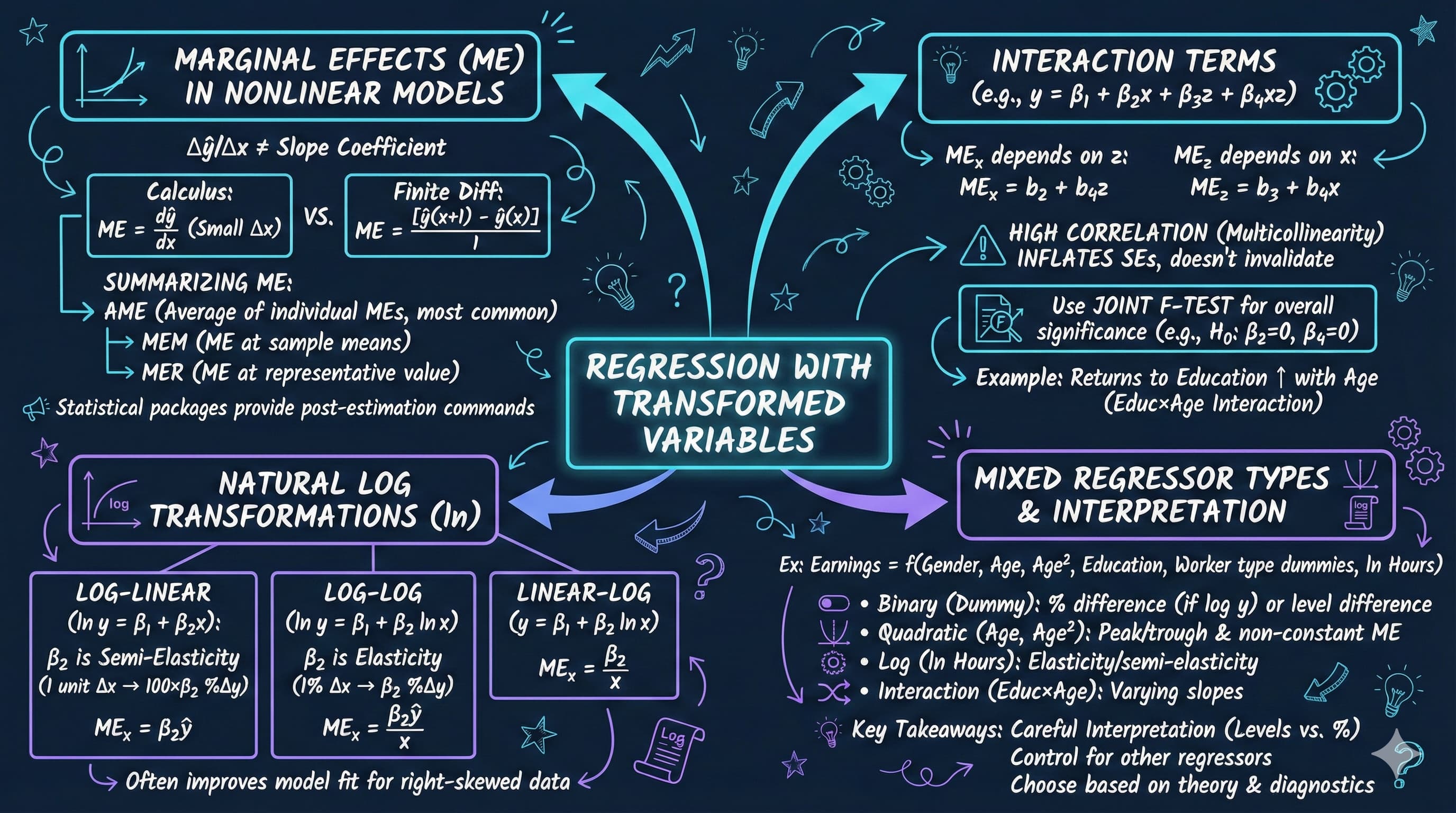
<img src="https://raw.githubusercontent.com/quarcs-lab/metricsai/main/images/ch15_visual_summary.jpg" alt="Chapter 15 Visual Summary" width="100%">
This notebook provides an interactive introduction to regression with transformed variables. All code runs directly in Google Colab without any local setup.
[](https://colab.research.google.com/github/quarcs-lab/metricsai/blob/main/notebooks_colab/ch15_Regression_with_Transformed_Variables.ipynb)
<div class="chapter-resources">
<a href="https://www.youtube.com/watch?v=XJv1bfr9BI4" target="_blank" class="resource-btn">🎬 AI Video</a>
<a href="https://carlos-mendez.my.canva.site/s15-regression-with-transformed-variables-pdf" target="_blank" class="resource-btn">✨ AI Slides</a>
<a href="https://cameron.econ.ucdavis.edu/aed/traedv1_15" target="_blank" class="resource-btn">📊 Cameron Slides</a>
<a href="https://app.edcafe.ai/quizzes/69786b142f5d08069e04d9ed" target="_blank" class="resource-btn">✏️ Quiz</a>
<a href="https://app.edcafe.ai/chatbots/6978a2c92f5d08069e072021" target="_blank" class="resource-btn">🤖 AI Tutor</a>
</div>
## Chapter Overview
This chapter focuses on regression models that involve transformed variables. Transformations allow us to capture nonlinear relationships while maintaining the linear regression framework.
**What you'll learn:**
- Understand how variable transformations affect regression interpretation
- Compute and interpret marginal effects for nonlinear models
- Distinguish between average marginal effects (AME), marginal effects at the mean (MEM), and marginal effects at representative values (MER)
- Estimate and interpret quadratic and polynomial regression models
- Work with interaction terms and test their joint significance
- Apply natural logarithm transformations to create log-linear and log-log models
- Make predictions from models with transformed dependent variables, avoiding retransformation bias
- Combine multiple types of variable transformations in a single model
**Dataset used:**
- **AED_EARNINGS_COMPLETE.DTA**: 872 workers aged 25-65 in 2000
**Key economic questions:**
- How do earnings vary with age? Is the relationship linear or quadratic?
- Do returns to education increase with age (interaction effects)?
- How should we interpret coefficients in log-transformed models?
- How do we make unbiased predictions from log-linear models?
**Chapter outline:**
- 15.1 Example - Earnings and Education
- 15.2 Logarithmic Transformations
- 15.3 Polynomial Regression (Quadratic Models)
- 15.4 Standardized Variables
- 15.5 Interaction Terms and Marginal Effects
- 15.6 Retransformation Bias and Prediction
- 15.7 Comprehensive Model with Mixed Regressors
- Key Takeaways
- Practice Exercises
- Case Studies
## Key Concepts
Seven core ideas anchor this chapter. Skim them before you start, and come back when a term feels fuzzy. Each entry pairs a concrete example using the chapter's data with a non-technical analogy. Click a panel to expand it.
**Marginal Effect:** The change in $y$ associated with a one-unit increase in a regressor, holding the other regressors fixed. In a plain linear model the marginal effect is just the slope; once $x$ enters the regression nonlinearly (squared, logged, interacted), the marginal effect varies with the value of $x$.
::::: {.columns}
:::: {.column width="50%"}
::: {.callout-tip collapse="true" appearance="simple" title="Example"}
For the 872 workers in `data_earnings`, the linear model gives a constant marginal effect of `age` of about \$525 per year. The chapter's quadratic fit replaces it with $ME_{\text{age}} = \beta_2 + 2\beta_3 \cdot \text{age}$ — about $+\$1{,}600$ at age 25, $\$0$ at the turning point near age 52, and $-\$450$ at age 60. Same regressor, very different marginal stories.
:::
::::
:::: {.column width="50%"}
::: {.callout-note collapse="true" appearance="simple" title="Analogy"}
The grade of a road tells you how much elevation you gain per metre walked *right here*. On a flat stretch the grade is zero; climbing a hill it is positive; rolling downhill it is negative. The marginal effect is the regression's road-grade — the slope you feel taking *one more step* in the regressor.
:::
::::
:::::
**Average Marginal Effect (AME):** Compute the marginal effect for *every* observation in the sample, then average. The AME summarises the typical marginal change across the whole population represented by the data, rather than the change at any one specific point.
::::: {.columns}
:::: {.column width="50%"}
::: {.callout-tip collapse="true" appearance="simple" title="Example"}
For the quadratic earnings-on-age model, $ME_{\text{age}, i} = \beta_2 + 2\beta_3 \cdot \text{age}_i$ is computed for each of the 872 workers and then averaged. The AME for `age` lands between the high-young-worker effect (+\$1{,}600) and the negative-old-worker effect (–\$450), giving a single summary number that respects the full age distribution in the sample.
:::
::::
:::: {.column width="50%"}
::: {.callout-note collapse="true" appearance="simple" title="Analogy"}
A symphony tracks the tempo at every bar across an entire performance, then reports the average. That single number is the *average tempo* — not the conductor's tempo at any one moment, but a faithful summary of how fast the orchestra played overall. AME is the regression's average-tempo statistic for a marginal effect that varies through the score.
:::
::::
:::::
**Marginal Effect at the Mean (MEM):** Plug the *sample-mean values* of every regressor into the marginal-effect formula and compute the resulting number. MEM tells you the marginal effect for a "representative average individual", which can differ noticeably from the AME when the marginal-effect curve is highly nonlinear.
::::: {.columns}
:::: {.column width="50%"}
::: {.callout-tip collapse="true" appearance="simple" title="Example"}
With the quadratic earnings-on-age fit, MEM is $\beta_2 + 2\beta_3 \cdot \overline{\text{age}}$ — using the chapter's mean `age` of about 43, giving a marginal effect of about $+\$536$ per year for the "average worker". For a *quadratic* model the marginal effect is linear in age, so here MEM equals the AME exactly; the two diverge only when the marginal-effect curve is itself nonlinear (as in logit or higher-order polynomial models).
:::
::::
:::: {.column width="50%"}
::: {.callout-note collapse="true" appearance="simple" title="Analogy"}
A photographer focuses the lens on the median guest at a wedding for a "representative" portrait. The result describes that one focused-on guest sharply — but says nothing about the kid at the corner table or the grandmother at the bar. MEM is the regression's "in-focus average guest": precise about that point, less informative about the spread.
:::
::::
:::::
**Marginal Effect at Representative Values (MER):** Plug *chosen* values of the regressors into the marginal-effect formula — typically a few policy-relevant profiles (a 25-year-old, a 40-year-old, a 55-year-old). MER lets you report several marginal effects, each tailored to a specific scenario.
::::: {.columns}
:::: {.column width="50%"}
::: {.callout-tip collapse="true" appearance="simple" title="Example"}
The chapter's interaction model `earnings ~ age + education + agebyeduc` reports $ME_{\text{education}}$ at three representative ages: $+\$5{,}241$ per education-year at age 25, $+\$5{,}677$ at age 40, and $+\$6{,}112$ at age 55 — only about a 1.2× change across the working life (and the underlying age×education interaction is not statistically significant, $p \approx 0.61$). These three MER values illuminate what AME and MEM each smooth over.
:::
::::
:::: {.column width="50%"}
::: {.callout-note collapse="true" appearance="simple" title="Analogy"}
A tailor doesn't make one suit for "the average customer"; they make one suit per customer profile — a tall slim athlete, a short stocky executive, a teenager. Each suit fits its target precisely. MER is the regression's bespoke-suit reporting: instead of one number, a small set of effects, each cut to a profile of interest.
:::
::::
:::::
**Polynomial Regression:** A regression that includes powers of a regressor — $x$, $x^2$, $x^3$, … — to capture curvature while keeping the model linear in coefficients. The quadratic form is the most common; cubic and higher add additional bends but invite over-fitting in small samples.
::::: {.columns}
:::: {.column width="50%"}
::: {.callout-tip collapse="true" appearance="simple" title="Example"}
The chapter fits `earnings ~ age + agesq + education` on `data_earnings`. The linear `age` coefficient is around $+\$3{,}000$ to $+\$5{,}000$ and the quadratic `agesq` coefficient is around $-\$30$ to $-\$50$ — together producing the inverted-U life-cycle pattern with peak earnings near age 50. The joint $F$-test on `age` and `agesq` is highly significant, ruling out the simpler linear-in-age model.
:::
::::
:::: {.column width="50%"}
::: {.callout-note collapse="true" appearance="simple" title="Analogy"}
A roller-coaster track climbs, peaks, dips, climbs again — its height isn't a straight line, but it can still be described by a smooth equation that bends in just the right places. Polynomial regression is the regression's roller-coaster: the relationship between $x$ and $y$ rises, peaks, falls — and the coefficients on $x, x^2, \dots$ are the engineering specs of the curve.
:::
::::
:::::
**Standardised Variable ($z$-score within a regression):** Replace each variable by $(x - \bar{x})/s_x$ before fitting. The resulting coefficients tell you the change in $y$ — measured in $y$'s standard deviations — for a one-standard-deviation change in $x$. Standardising puts variables in different units onto a common scale, useful when comparing relative importance.
::::: {.columns}
:::: {.column width="50%"}
::: {.callout-tip collapse="true" appearance="simple" title="Example"}
In the chapter's mixed-regressor earnings model (`earnings ~ gender + age + agesq + education + dself + dgovt + lnhours`), the raw coefficient on `lnhours` (in dollars per log-hour) cannot be compared directly to the coefficient on `education` (in dollars per year). Standardising both produces $\beta^*$ values that *can* be compared: who moves earnings more, by one SD of effort? Age and its squared term come out as the largest standardised effects; among the remaining regressors, education and `lnhours` have the largest standardised coefficients.
:::
::::
:::: {.column width="50%"}
::: {.callout-note collapse="true" appearance="simple" title="Analogy"}
A currency converter restates a price in dollars, euros, and yen on a single line so you can compare what each pays you for the same coffee. Standardisation does the same for regressors: it converts dollars-per-year, hours-per-week, and binary flags into a common "standard-deviation" currency, so each coefficient is finally comparable to the others.
:::
::::
:::::
**Smearing Estimator (Duan's):** A nonparametric correction for retransformation bias when the dependent variable is logged. Instead of multiplying $\exp(\widehat{\ln y})$ by a normality-based factor like $\exp(s_e^2/2)$, Duan's method multiplies by the empirical mean $\tfrac{1}{n}\sum \exp(\hat{u}_i)$ — letting the residuals themselves correct the bias.
::::: {.columns}
:::: {.column width="50%"}
::: {.callout-tip collapse="true" appearance="simple" title="Example"}
For the log-linear earnings model on `data_earnings` ($s_e \approx 0.62$), naive retransformation $\exp(\widehat{\ln y})$ gives a sample-mean prediction of about \$46k — well below the actual mean of \$56k. The normality-based factor $\exp(0.62^2/2) \approx 1.21$ recovers about \$55k; Duan's smearing correction averages $\exp(\hat{u}_i)$ across the 872 residuals to produce essentially the same correction without assuming normality.
:::
::::
:::: {.column width="50%"}
::: {.callout-note collapse="true" appearance="simple" title="Analogy"}
A cook prepares a recipe and finds the salt always measures slightly low at the end. Rather than use a textbook formula to compute the missing pinch, the smearing approach is to look back at the *actual* leftover residue from past batches and add exactly that average back in. The salt comes out right because the correction is read from real cooking, not theory.
:::
::::
:::::
## Setup
First, we import the necessary Python packages and configure the environment for reproducibility. All data will stream directly from GitHub.
```{python}
#| code-fold: true
#| code-summary: "Setup: Import libraries and configure environment"
# --- Libraries ---
import numpy as np                        # numerical operations
import pandas as pd                       # data manipulation
import matplotlib.pyplot as plt           # plotting
import seaborn as sns                     # statistical plots
import pyfixest as pf                    # fast OLS estimation
from scipy import stats                   # statistical distributions
import random
import os

# --- Reproducibility ---
RANDOM_SEED = 42
random.seed(RANDOM_SEED)
np.random.seed(RANDOM_SEED)
os.environ['PYTHONHASHSEED'] = str(RANDOM_SEED)

# --- Data source ---
GITHUB_DATA_URL = "https://raw.githubusercontent.com/quarcs-lab/data-open/master/AED/"

# --- Plotting style (dark theme matching book design) ---
plt.style.use('dark_background')
sns.set_style("darkgrid")
plt.rcParams.update({
    'axes.facecolor': '#1a2235',
    'figure.facecolor': '#12162c',
    'grid.color': '#3a4a6b',
    'figure.figsize': (10, 6),
    'text.color': 'white',
    'axes.labelcolor': 'white',
    'xtick.color': 'white',
    'ytick.color': 'white',
    'axes.edgecolor': '#1a2235',
})
```
## 15.1 Example - Earnings and Education
We'll work with the EARNINGS_COMPLETE dataset, which contains information on 872 female and male full-time workers aged 25-65 years in 2000.
**Key variables:**
- **earnings**: Annual earnings in dollars
- **lnearnings**: Natural logarithm of earnings
- **age**: Age in years
- **agesq**: Age squared
- **education**: Years of schooling
- **agebyeduc**: Age × Education interaction
- **gender**: 1 if female, 0 if male
- **dself**: 1 if self-employed
- **dgovt**: 1 if government sector employee
- **lnhours**: Natural logarithm of hours worked per week
```{python}
# Read in the earnings data
data_earnings = pd.read_stata(GITHUB_DATA_URL + 'AED_EARNINGS_COMPLETE.DTA')

print("Data structure:")
data_earnings.info()

print("\nData summary:")
data_summary = data_earnings.describe()
print(data_summary)

print("\nFirst few observations:")
key_vars = ['earnings', 'lnearnings', 'age', 'agesq', 'education', 'agebyeduc',
            'gender', 'dself', 'dgovt', 'lnhours']
data_earnings[key_vars].head(10)
```
## 15.2 Logarithmic Transformations
Logarithmic transformations are commonly used in economics because:
1. They can linearize multiplicative relationships
2. Coefficients have natural interpretations (percentages, elasticities)
3. They reduce the influence of outliers
4. They often make error distributions more symmetric
**Three main types of log models:**
1. **Levels model**: $y = \beta_1 + \beta_2 x + u$
- Interpretation: $\Delta y = \beta_2 \Delta x$
2. **Log-linear model**: $\ln y = \beta_1 + \beta_2 x + u$
- Interpretation: A one-unit increase in $x$ leads to approximately \$100\beta_2\%$ change in $y$
- Also called semi-elasticity
3. **Log-log model**: $\ln y = \beta_1 + \beta_2 \ln x + u$
- Interpretation: A 1% increase in $x$ leads to $\beta_2\%$ change in $y$
- $\beta_2$ is an elasticity
**Marginal effects:**
- Log-linear: $ME_x = \beta_2 \times y$
- Log-log: $ME_x = \beta_2 \times y / x$
```{python}
# Create ln(age) variable if not already present
if 'lnage' not in data_earnings.columns:
    data_earnings['lnage'] = np.log(data_earnings['age'])
    print("Created lnage variable")
else:
    print("lnage already exists")
```
```{python}
# 15.2 Logarithmic Transformations

# Model 1: Levels Model - earnings ~ age + education
fit_linear = pf.feols('earnings ~ age + education', data=data_earnings, vcov='HC1')

# Model 2: Log-Linear Model - lnearnings ~ age + education
fit_loglin = pf.feols('lnearnings ~ age + education', data=data_earnings, vcov='HC1')

# Model 3: Log-Log Model - lnearnings ~ lnage + education
fit_loglog = pf.feols('lnearnings ~ lnage + education', data=data_earnings, vcov='HC1')

# Key results across all three specifications
print("=== Model 1: Levels ===")
print(f"  Equation: earnings = {fit_linear.coef()['Intercept']:,.0f} + {fit_linear.coef()['age']:.2f} x age + {fit_linear.coef()['education']:.2f} x education")
print(f"  R-squared: {fit_linear._r2:.4f}")

print("\n=== Model 2: Log-Linear ===")
print(f"  Equation: ln(earnings) = {fit_loglin.coef()['Intercept']:.4f} + {fit_loglin.coef()['age']:.4f} x age + {fit_loglin.coef()['education']:.4f} x education")
print(f"  Education return: ~{100*fit_loglin.coef()['education']:.1f}% per year (semi-elasticity)")
print(f"  R-squared: {fit_loglin._r2:.4f}")

print("\n=== Model 3: Log-Log ===")
print(f"  Equation: ln(earnings) = {fit_loglog.coef()['Intercept']:.4f} + {fit_loglog.coef()['lnage']:.4f} x ln(age) + {fit_loglog.coef()['education']:.4f} x education")
print(f"  Age elasticity: {fit_loglog.coef()['lnage']:.4f} (a 1% increase in age -> {fit_loglog.coef()['lnage']:.2f}% increase in earnings)")
print(f"  R-squared: {fit_loglog._r2:.4f}")

# Full regression output (Model 2 - the Mincer equation)
fit_loglin.summary()
```
> **Key Concept 15.1: Log Transformations and Coefficient Interpretation**
>
> In a **log-linear model** ($\ln y = \beta_1 + \beta_2 x$), the coefficient $\beta_2$ is a semi-elasticity: a 1-unit increase in $x$ is associated with approximately a $100 \times \beta_2$% change in $y$ (the exact effect is $100(e^{\beta_2}-1)$%, which matters once $|\beta_2| > 0.1$). In a **log-log model** ($\ln y = \beta_1 + \beta_2 \ln x$), the coefficient $\beta_2$ is an elasticity: a 1% increase in $x$ is associated with a $\beta_2$% change in $y$.
### Interpretation of Log Models
Let's carefully interpret the coefficients from each model.
---
#### Understanding Elasticities and Percentage Changes
The three models reveal fundamentally different ways to think about the relationship between earnings, age, and education. Let's interpret each carefully:
**Model 1: Levels (earnings ~ age + education)**
- **Age coefficient** ≈ \$525 per year
- Interpretation: Each additional year of age increases earnings by approximately **\$525**
- This is an **absolute change** measured in dollars
- Assumes **constant** effect regardless of current age or earnings level
- **Education coefficient** ≈ \$4,000-\$6,000 per year
- Interpretation: Each additional year of schooling increases earnings by approximately **\$5,000**
- Again, this is an **absolute dollar amount**
- Assumes the same dollar return whether you have 10 or 20 years of education
**Model 2: Log-Linear (ln(earnings) ~ age + education)**
- **Age coefficient** ≈ 0.008
- Interpretation: Each additional year of age increases earnings by approximately **0.8%**
- This is a **percentage change** (semi-elasticity)
- The **dollar impact depends on current earnings**
- For someone earning \$50,000: 0.8% × \$50,000 = \$400
- For someone earning \$100,000: 0.8% × \$100,000 = \$800
- **Education coefficient** ≈ 0.08 to 0.12
- Interpretation: Each additional year of education increases earnings by approximately **8-12%**
- This is the famous **Mincer return to education**
- Classic labor economics result: education yields ~10% return per year
- Percentage effect, so dollar gain is larger for high earners
**Model 3: Log-Log (ln(earnings) ~ ln(age) + education)**
- **ln(Age) coefficient** ≈ 0.35
- Interpretation: A **1% increase in age** increases earnings by approximately **0.35%**
- This is an **elasticity** (percentage change in Y for 1% change in X)
- Elasticity < 1 means **inelastic** relationship (earnings increase slower than age)
- At age 40: 1% increase = 0.4 years; at age 50: 1% increase = 0.5 years
- **Education coefficient** ≈ 0.08 to 0.12 (similar to log-linear)
- Education enters in levels, so interpretation same as Model 2
- Each additional year → ~10% increase in earnings
**Which Model to Choose?**
1. **Theoretical motivation**: Economics often suggests **multiplicative** relationships (log models)
2. **Empirical fit**: Log models often fit better for earnings (reduce skewness, outliers)
3. **Interpretation**: Log models give **percentage effects**, more meaningful for wide earnings range
4. **Heteroskedasticity**: Log transformation often reduces heteroskedasticity
**Key Insight:**
- The **Mincer equation** (log-linear) is standard in labor economics
- Returns to education are approximately **10% per year** across many countries and time periods
- This is one of the most robust findings in empirical economics!
### Comparison Table and Model Selection
```{python}
# Create comparison table
# MODEL COMPARISON: Levels, Log-Linear, and Log-Log

comparison_table = pd.DataFrame({
    'Model': ['Levels', 'Log-Linear', 'Log-Log'],
    'Specification': ['earnings ~ age + education',
                      'ln(earnings) ~ age + education',
                      'ln(earnings) ~ ln(age) + education'],
    'R-squared': [fit_linear._r2, fit_loglin._r2, fit_loglog._r2],
    'Adj R-squared': [fit_linear._adj_r2, fit_loglin._adj_r2, fit_loglog._adj_r2]
})

print(comparison_table.to_string(index=False))

print("\nNote: R² values are NOT directly comparable across models with different")
# dependent variables. For log models, R² measures fit to ln(earnings), not earnings.
```
> **Key Concept 15.2: Choosing Between Model Specifications**
>
> You cannot directly compare $R^2$ across models with different dependent variables ($y$ vs $\ln y$) because they measure variation on different scales. Instead, compare models using **prediction accuracy** (e.g., mean squared error of predicted $y$ in levels), information criteria (AIC, BIC), or economic plausibility of the estimated relationships.
## 15.3 Polynomial Regression (Quadratic Models)
Polynomial regression allows for nonlinear relationships while maintaining linearity in parameters.
**Quadratic model:**
$$y = \beta_1 + \beta_2 x + \beta_3 x^2 + u$$
**Properties:**
- If $\beta_3 < 0$: inverted U-shape (peaks then declines)
- If $\beta_3 > 0$: U-shape (declines then increases)
- Turning point at $x^* = -\beta_2 / (2\beta_3)$
**Marginal effect:**
$$ME_x = \frac{\partial y}{\partial x} = \beta_2 + 2\beta_3 x$$
**Average marginal effect (AME):**
$$AME = \beta_2 + 2\beta_3 \bar{x}$$
**Statistical significance of age:**
- Must test jointly: $H_0: \beta_{age} = 0$ AND $\beta_{agesq} = 0$
- Individual t-tests are insufficient
```{python}
# 15.3 Polynomial Regression (Quadratic Models)

# Linear model (for comparison)
# Linear Model: earnings ~ age + education
fit_linear_age = pf.feols('earnings ~ age + education', data=data_earnings, vcov='HC1')

# Quadratic Model: earnings ~ age + agesq + education
fit_quad = pf.feols('earnings ~ age + agesq + education', data=data_earnings, vcov='HC1')

# Key results: Quadratic vs Linear
print(f"Linear model R-squared:    {fit_linear_age._r2:.4f}")
print(f"Quadratic model R-squared: {fit_quad._r2:.4f}")
print(f"\nQuadratic coefficients:")
print(f"  age:       {fit_quad.coef()['age']:,.2f}")
print(f"  age-sq:    {fit_quad.coef()['agesq']:.4f}")
print(f"  education: {fit_quad.coef()['education']:,.2f}")

# Full regression output (quadratic model)
fit_quad.summary()
```
With the quadratic fit in hand, we extract its economic content: the age at which earnings peak (the turning point) and the marginal effect of age evaluated at several representative ages. Watch how the marginal effect starts large and positive for young workers and turns negative once age passes the turning point.
```{python}
# TURNING POINT AND MARGINAL EFFECTS

# Extract coefficients
bage = fit_quad.coef()['age']
bagesq = fit_quad.coef()['agesq']
beducation = fit_quad.coef()['education']

# Calculate turning point
turning_point = -bage / (2 * bagesq)

print(f"\nTurning Point:")
print(f"  Age at maximum earnings: {turning_point:.1f} years")

# Marginal effects at different ages
ages_to_eval = [25, 40, 55, 65]
print(f"\nMarginal Effect of Age on Earnings:")
for age in ages_to_eval:
    me = bage + 2 * bagesq * age
    print(f"  At age {age}: ${me:,.2f} per year")

# Average marginal effect
mean_age = data_earnings['age'].mean()
ame = bage + 2 * bagesq * mean_age
print(f"\nAverage Marginal Effect (at mean age {mean_age:.1f}): ${ame:,.2f}")
```
> **Key Concept 15.3: Quadratic Models and Turning Points**
>
> A quadratic model $y = \beta_1 + \beta_2 x + \beta_3 x^2 + u$ captures nonlinear relationships with a **turning point** at $x^* = -\beta_2 / (2\beta_3)$. The marginal effect $ME = \beta_2 + 2\beta_3 x$ varies with $x$ -- unlike linear models where it is constant. If $\beta_3 < 0$, the relationship is an inverted U-shape (e.g., earnings peaking at a certain age).
### Quadratic Model: Turning Point and Marginal Effects
---
#### Life-Cycle Earnings Profile: The Inverted U-Shape
The quadratic model reveals a fundamental pattern in labor economics - the **inverted U-shaped age-earnings profile**. Let's understand what the results tell us:
**Interpreting the Quadratic Coefficients:**
From the regression: earnings = $\beta_1 + \beta_2 \cdot age + \beta_3 \cdot age^2 + \beta_4 \cdot education + u$
**Typical Results:**
- **Age coefficient** ($\beta_2$) ≈ **+\$3,000 to +\$5,000** (positive, large)
- **Age² coefficient** ($\beta_3$) ≈ **-\$30 to -\$50** (negative, small)
**What does this mean?**
1. **The Turning Point** (Peak Earnings Age):
- Formula: $age^* = -\beta_2 / (2\beta_3)$
- Typical result: **age 45-55 years**
- Interpretation: Earnings **increase** until age 50, then **decline**
- This matches real-world patterns: mid-career workers earn most
2. **Marginal Effect of Age** (varies with age):
- Formula: $ME_{age} = \beta_2 + 2\beta_3 \cdot age$
- At age 25: ME ≈ +\$1,600 (steep increase)
- At age 40: ME ≈ +\$700 (slower increase)
- At age 50: ME ≈ \$0 (peak earnings)
- At age 60: ME ≈ -\$450 (earnings decline)
3. **Why the Inverted U-Shape?**
- **Early career (20s-30s)**: Rapid skill accumulation, promotions → steep earnings growth
- **Mid-career (40s-50s)**: Peak productivity, seniority → highest earnings
- **Late career (55+)**: Reduced hours, health decline, obsolete skills → earnings fall
- Human capital theory: Investment in skills early, returns later, depreciation at end
**Comparing Linear vs. Quadratic:**
- **Linear model**: Assumes constant age effect (+\$525/year regardless of age)
- Misses the fact that earnings growth **slows down** and eventually **reverses**
- Poor fit for older workers
- **Quadratic model**: Captures realistic life-cycle pattern
- Allows for **increasing, then decreasing** returns to age
- Better fit (higher R²)
- More accurate predictions for both young and old workers
**Statistical Significance:**
The **joint F-test** for $H_0: \beta_{age} = 0$ AND $\beta_{age^2} = 0$ is **highly significant** (F ≈ 19, p < 0.001):
- This confirms age **matters** for earnings
- The quadratic term is **necessary** (not just linear)
- Individual t-tests can be misleading due to collinearity between age and age²
**Economic Implications:**
- Peak earnings around age 50 suggests optimal **retirement age** discussions
- Earnings decline after 55 may incentivize early retirement
- Policy relevance for Social Security, pension design
- Training investments more valuable early in career
### Joint Hypothesis Test for Quadratic Term
```{python}
# Joint hypothesis test: H0: age = 0 and agesq = 0
# JOINT HYPOTHESIS TEST: H₀: β_age = 0 AND β_agesq = 0

hypotheses = '(age = 0, agesq = 0)'
f_test = fit_quad.wald_test(R=np.eye(len(fit_quad.coef()))[[list(fit_quad.coef().index).index(v) for v in ['age', 'agesq']]])
print(f_test)

print("\nInterpretation:")
if f_test.pvalue < 0.05:
    # Reject H₀: Age is jointly statistically significant in the model.
    print("  The quadratic specification is justified.")
else:
    # Fail to reject H₀: Age is not statistically significant.
    print("  The quadratic specification is not justified.")
```
> **Key Concept 15.4: Testing Nonlinear Relationships**
>
> When a quadratic term $x^2$ is included, always test the **joint significance** of $x$ and $x^2$ together using an F-test. Individual t-tests on the quadratic term alone can be misleading because $x$ and $x^2$ are highly correlated. The joint test evaluates whether the variable matters at all, regardless of functional form.
### Visualization: Quadratic Relationship
```{python}
# Create visualization of quadratic relationship
fig, axes = plt.subplots(1, 2, figsize=(16, 6))

# Left plot: Fitted values vs age
age_range = np.linspace(25, 65, 100)
educ_mean = data_earnings['education'].mean()

# Predictions holding education at mean
linear_pred = fit_linear_age.coef()['Intercept'] + fit_linear_age.coef()['age']*age_range + fit_linear_age.coef()['education']*educ_mean
quad_pred = fit_quad.coef()['Intercept'] + bage*age_range + bagesq*age_range**2 + beducation*educ_mean

axes[0].scatter(data_earnings['age'], data_earnings['earnings'], alpha=0.3, s=20, color='gray', label='Actual data')  # alpha = transparency, s = marker size
axes[0].plot(age_range, linear_pred, '-', color='#c084fc', linewidth=2, label='Linear model')
axes[0].plot(age_range, quad_pred, 'r-', linewidth=2, label='Quadratic model')
axes[0].axvline(x=turning_point, color='green', linestyle='--', linewidth=1.5, alpha=0.7, label=f'Turning point ({turning_point:.1f} years)')
axes[0].set_xlabel('Age (years)', fontsize=12)
axes[0].set_ylabel('Earnings ($)', fontsize=12)
axes[0].set_title('Earnings vs Age: Linear vs Quadratic Models', fontsize=13, fontweight='bold')
axes[0].legend()
axes[0].grid(True, alpha=0.3)

# Right plot: Marginal effects
me_linear = np.full_like(age_range, fit_linear_age.coef()['age'])
me_quad = bage + 2 * bagesq * age_range

axes[1].plot(age_range, me_linear, '-', color='#c084fc', linewidth=2, label='Linear model (constant)')
axes[1].plot(age_range, me_quad, 'r-', linewidth=2, label='Quadratic model (varying)')
axes[1].axhline(y=0, color='white', alpha=0.3, linestyle='-', linewidth=0.8)
axes[1].axvline(x=turning_point, color='green', linestyle='--', linewidth=1.5, alpha=0.7, label=f'Turning point ({turning_point:.1f} years)')
axes[1].fill_between(age_range, 0, me_quad, where=(me_quad > 0), alpha=0.2, color='green', label='Positive effect')
axes[1].fill_between(age_range, 0, me_quad, where=(me_quad < 0), alpha=0.2, color='red', label='Negative effect')
axes[1].set_xlabel('Age (years)', fontsize=12)
axes[1].set_ylabel('Marginal Effect on Earnings ($)', fontsize=12)
axes[1].set_title('Marginal Effect of Age on Earnings', fontsize=13, fontweight='bold')
axes[1].legend()
axes[1].grid(True, alpha=0.3)

plt.tight_layout()
plt.show()

# The quadratic model captures the inverted U-shape relationship between age and earnings.
```
**What to look for in this quadratic visualization:**
- **Left panel**: The quadratic (red) curve bends downward after the turning point, capturing the earnings decline at older ages that the linear model (purple) misses entirely
- **Turning point**: The green dashed line marks the age where additional years stop increasing earnings -- a key policy-relevant quantity
- **Right panel**: The marginal effect of age decreases steadily; the green/red shading shows where an extra year of age helps vs. hurts earnings
## 15.4 Standardized Variables
Standardized regression coefficients (beta coefficients) allow comparison of the relative importance of regressors measured in different units.
**Standardization formula:**
$$z_x = \frac{x - \bar{x}}{s_x}$$
where $s_x$ is the standard deviation of $x$.
**Standardized coefficient:**
$$\beta^* = \beta \times \frac{s_x}{s_y}$$
**Interpretation:**
- $\beta^*$ shows the effect of a one-standard-deviation change in $x$ on $y$, measured in standard deviations of $y$
- Allows comparison: which variable has the largest effect when measured in comparable units?
**Use cases:**
- Comparing effects of variables with different units
- Meta-analysis across studies
- Understanding relative importance of predictors
```{python}
# 15.4 Standardized Variables

# Estimate a comprehensive model
# Linear Model with Mixed Regressors:
# earnings ~ gender + age + agesq + education + dself + dgovt + lnhours
fit_linear_mix = pf.feols('earnings ~ gender + age + agesq + education + dself + dgovt + lnhours',
                     data=data_earnings, vcov='HC1')

# Key results
print(f"R-squared: {fit_linear_mix._r2:.4f} ({fit_linear_mix._r2*100:.1f}% of variation explained)")
print(f"Education: +${fit_linear_mix.coef()['education']:,.0f} per year of schooling")
print(f"Gender: ${fit_linear_mix.coef()['gender']:,.0f} (negative = women earn less)")

# Full regression output
fit_linear_mix.summary()
```
The raw coefficients above are measured in different units (dollars per year, dollars per log-hour, dollars per dummy), so their magnitudes are not directly comparable. Next we rescale each coefficient into standard-deviation units. Look for which variable has the largest absolute standardized coefficient -- that is the strongest predictor on a common scale.
```{python}
# STANDARDIZED COEFFICIENTS

# Get standard deviations
sd_y = data_earnings['earnings'].std()
sd_gender = data_earnings['gender'].std()
sd_age = data_earnings['age'].std()
sd_agesq = data_earnings['agesq'].std()
sd_education = data_earnings['education'].std()
sd_dself = data_earnings['dself'].std()
sd_dgovt = data_earnings['dgovt'].std()
sd_lnhours = data_earnings['lnhours'].std()

# Calculate standardized coefficients
standardized_coefs = {
    'gender': fit_linear_mix.coef()['gender'] * sd_gender / sd_y,
    'age': fit_linear_mix.coef()['age'] * sd_age / sd_y,
    'agesq': fit_linear_mix.coef()['agesq'] * sd_agesq / sd_y,
    'education': fit_linear_mix.coef()['education'] * sd_education / sd_y,
    'dself': fit_linear_mix.coef()['dself'] * sd_dself / sd_y,
    'dgovt': fit_linear_mix.coef()['dgovt'] * sd_dgovt / sd_y,
    'lnhours': fit_linear_mix.coef()['lnhours'] * sd_lnhours / sd_y
}

print("\nStandardized Coefficients (Beta coefficients):")
for var, beta in sorted(standardized_coefs.items(), key=lambda x: abs(x[1]), reverse=True):
    print(f"  {var:12s}: {beta:7.4f}")

print("\nInterpretation:")
# These show the effect of a 1 SD change in X on Y (in SD units)
print("  Allows comparison of relative importance across variables")
```
> **Key Concept 15.5: Standardized Coefficients for Comparing Variable Importance**
>
> Standardized (beta) coefficients $\beta^* = \beta \times (s_x / s_y)$ measure effects in **standard deviation units**, allowing comparison across variables with different scales. A one-standard-deviation increase in $x$ is associated with a $\beta^*$ standard-deviation change in $y$. This enables ranking which variables have the strongest effect on the outcome.
### Calculate Standardized Coefficients
---
#### Comparing Apples to Apples: Standardized Coefficients
Standardized coefficients allow us to answer: **"Which variable matters most for earnings?"**
**The Problem with Raw Coefficients:**
Looking at the regression:
- Education: +\$5,000 per year
- Age: +\$1,000 per year
- Hours: +\$500 per hour
Can we conclude education is "most important"? **Not necessarily!**
- These variables are measured in **different units**
- Education varies from 8 to 20 years (SD ≈ 2-3 years)
- Age varies from 25 to 65 years (SD ≈ 10-12 years)
- Hours varies from 35 to 60 per week (SD ≈ 8-10 hours)
**The Solution: Standardized (Beta) Coefficients**
Transform to: **"What if all variables were measured in standard deviations?"**
Formula: $\beta^* = \beta \times (SD_x / SD_y)$
**Interpretation:**
- A 1 SD increase in X leads to $\beta^*$ SD change in Y
- Now all variables are **comparable** (measured in same units)
**Results from the Analysis:**
Ranking by absolute standardized coefficients (largest to smallest):
1. **Age and Age²** ($\beta^* \approx +0.68$ and $-0.57$):
- The **largest standardized coefficients** in this model
- Read them together: `age` and `agesq` are the two halves of one quadratic term, so their individual $\beta^*$ values partly offset and overstate age's standalone importance
- Age still matters most on a common scale, but through its nonlinear life-cycle shape
2. **Education** ($\beta^* \approx 0.30$):
- The **strongest single continuous predictor** once the age/age² pair is set aside
- 1 SD increase in education (≈2.9 years) → 0.30 SD increase in earnings
- Consistent with human capital theory
3. **Hours worked** ($\beta^* \approx 0.22$):
- 1 SD increase in `lnhours` → 0.22 SD increase in earnings
- Makes sense: more hours → proportionally more pay
4. **Gender** ($\beta^* \approx -0.14$):
- **Substantial negative effect**
- Being female → about a 0.14 SD decrease in earnings
- This standardizes the raw gap of ~\$14,000
5. **Employment type** (dself, dgovt) ($\beta^* \approx 0.05$ and $0.00$):
- **Smaller effects**
- Self-employment carries a modest positive $\beta^*$; the government dummy is essentially zero
- Once we control for education, age, and hours
**Key Insights:**
1. **Age carries the largest standardized coefficients**: but `age` and `agesq` share the variance of one quadratic term, so read their $\beta^*$ values together rather than as independent effects
2. **Education is the strongest single predictor**: once the age/age² terms are set aside, supporting human capital theory
3. **Hours worked matters**: direct relationship (more work → more pay)
4. **Categorical variables** (gender, employment type) are also standardizable
**When to Use Standardized Coefficients:**
**Good for:**
- Comparing relative importance of predictors
- Meta-analysis across studies
- Understanding which variables to prioritize in data collection
**Not good for:**
- Policy analysis (need actual units for cost-benefit)
- Prediction (use original coefficients)
- Variables with naturally meaningful units (e.g., dummy variables)
**Caution:**
- Standardized coefficients depend on **sample variation**
- If your sample has little variation in X, $\beta^*$ will be small
- Different samples → different standardized coefficients
- Raw coefficients more stable across samples
### Visualization: Standardized Coefficients
```{python}
# Create visualization comparing standardized coefficients
fig, ax = plt.subplots(figsize=(10, 7))
vars_plot = list(standardized_coefs.keys())
betas_plot = list(standardized_coefs.values())

colors = ['red' if b < 0 else '#22d3ee' for b in betas_plot]
bars = ax.barh(vars_plot, betas_plot, color=colors, alpha=0.7)

ax.axvline(x=0, color='white', alpha=0.3, linestyle='-', linewidth=0.8)
ax.set_xlabel('Standardized Coefficient (SD units)', fontsize=12)
ax.set_ylabel('Variable', fontsize=12)
ax.set_title('Standardized Regression Coefficients\n(Effect of 1 SD change in X on Y, in SD units)',
             fontsize=14, fontweight='bold')
ax.grid(True, alpha=0.3, axis='x')

plt.tight_layout()
plt.show()
```
**What to look for in this standardized coefficient chart:**
- **Longest bars**: The variables with the largest absolute standardized coefficients are the strongest predictors of earnings when measured on a common scale
- **Direction (color)**: Cyan bars indicate positive effects; red bars indicate negative effects (e.g., gender penalty)
- **Relative ranking**: Compare education vs. hours vs. age -- the raw coefficients may suggest a different ranking because those variables are measured in different units
## 15.5 Interaction Terms and Marginal Effects
Interaction terms allow the marginal effect of one variable to depend on the level of another variable.
**Model with interaction:**
$$y = \beta_1 + \beta_2 x + \beta_3 z + \beta_4 (x \times z) + u$$
**Marginal effect of $x$:**
$$ME_x = \beta_2 + \beta_4 z$$
**Marginal effect of $z$:**
$$ME_z = \beta_3 + \beta_4 x$$
**Important:**
- Individual t-tests on $\beta_2$ or $\beta_4$ are misleading
- Test significance of $x$ jointly: $H_0: \beta_2 = 0$ AND $\beta_4 = 0$
- Interaction variables are often highly correlated with main effects (multicollinearity)
```{python}
# 15.5 Interaction Terms And Marginal Effects

# Model without interaction (for comparison)
# Model WITHOUT Interaction: earnings ~ age + education
fit_no_interact = pf.feols('earnings ~ age + education', data=data_earnings, vcov='HC1')

# Model WITH Interaction: earnings ~ age + education + agebyeduc
fit_interact = pf.feols('earnings ~ age + education + agebyeduc', data=data_earnings, vcov='HC1')

# Key results: How returns to education vary with age
b_educ = fit_interact.coef()['education']
b_inter = fit_interact.coef()['agebyeduc']
print(f"Interaction model: ME of education = {b_educ:,.0f} + {b_inter:.1f} x age")
print(f"  At age 25: ${b_educ + b_inter*25:,.0f} per year of education")
print(f"  At age 40: ${b_educ + b_inter*40:,.0f} per year of education")
print(f"  At age 55: ${b_educ + b_inter*55:,.0f} per year of education")
print(f"R-squared (with interaction): {fit_interact._r2:.4f}")

# Full regression output
fit_interact.summary()
```
> **Key Concept 15.6: Interaction Terms and Varying Marginal Effects**
>
> With an interaction term $x \times z$, the marginal effect of $x$ depends on $z$: $ME_x = \beta_2 + \beta_4 z$. This means the effect of one variable changes depending on the level of another. Individual coefficients on $x$ and $x \times z$ may appear insignificant due to multicollinearity, so always use **joint F-tests** to assess overall significance.
### Interaction Model: Marginal Effects and Joint Tests
---
#### How Returns to Education Change with Age
The interaction model asks whether the **payoff to education depends on age**. As we will see, in this sample the estimated dependence is small and statistically insignificant -- a useful cautionary example about not over-reading an interaction term.
**Interpreting the Interaction Results:**
From: earnings = $\beta_1 + \beta_2 \cdot age + \beta_3 \cdot education + \beta_4 \cdot (age \times education) + u$
**Typical Coefficients:**
- Education ($\beta_3$): About **+\$4,515** (positive; only marginally significant, p ≈ 0.06)
- Age × Education ($\beta_4$): About **+\$29** per year (small and statistically insignificant, p ≈ 0.61)
**What This Means:**
The marginal effect of education is:
$$ME_{education} = \beta_3 + \beta_4 \cdot age$$
**At Different Ages:**
- **Age 25**: ME ≈ \$4,515 + \$29(25) = **+\$5,241** per year of education
- **Age 40**: ME ≈ \$4,515 + \$29(40) = **+\$5,677** per year of education
- **Age 55**: ME ≈ \$4,515 + \$29(55) = **+\$6,112** per year of education
**Interpretation:**
1. **Returns to education barely change with age in this sample**
- Young workers (age 25): +\$5,241 per year of education
- Older workers (age 55): +\$6,112 per year of education
- The interaction coefficient is small (+\$29/year) and statistically insignificant (t = 0.5, p = 0.61), so there is no reliable evidence that the return to schooling rises with age here.
2. **Should we read into the small upward slope?**
- No -- because the interaction is statistically insignificant (p ≈ 0.61), the slight rise in estimated returns is well within sampling noise
- Mechanisms one might invoke for genuinely rising returns -- complementarity between education and experience, steeper career ladders, compounding raises -- are plausible stories, but this sample offers no reliable evidence that they operate here
3. **What the data do support**:
- Education has a large, positive average return (about +\$5,000 to +\$6,000 per year of schooling across the age range)
- What the data do *not* support is the stronger claim that this return climbs steeply with age
**Statistical Significance:**
- **Individual coefficients** may have large SEs (multicollinearity between age, education, and their product)
- **Joint F-test** is crucial: Test $H_0: \beta_{education} = 0$ AND $\beta_{age \times educ} = 0$
- Result: **Highly significant** (joint $\chi^2 \approx 86$, p < 0.001)
- This joint test confirms only that **education matters overall** -- it does *not* establish that education's effect varies with age. The age×education interaction is itself insignificant (t = 0.5, p ≈ 0.61), so there is no reliable evidence of age-dependence here.
**Multicollinearity Warning:**
The correlation matrix shows:
- Corr(age, age×education) ≈ **0.73** (high)
- Corr(education, age×education) ≈ **0.64** (moderately high)
This explains why:
- Individual t-statistics may be **small** (large SEs)
- Coefficients **sensitive** to small changes in data
- But joint tests **remain powerful**
**Policy Implications:**
1. **Education is a strong investment at every stage of the career**
- Short-run costs, long-run gains
- The average return is large and positive (~\$5,000-\$6,000 per year of schooling)
2. **Education pays off across the whole career**
- Adult education programs and retraining can have large payoffs
- The return does not reliably rise or fall with age in this sample
3. **Inequality implications**
- Education is a persistent source of earnings differences at every age
- Whether the education wage gap **widens** with age cannot be established here, since the age×education interaction is insignificant
**Practical Advice for Estimation:**
**Do:**
- Always test interactions **jointly** with main effects
- Report F-statistics for joint tests
- Calculate marginal effects at **representative ages** (25, 40, 55)
- Plot the relationship to visualize
**Don't:**
- Rely on individual t-tests when variables are highly correlated
- Drop the main effect if interaction is "insignificant"
- Interpret the main effect coefficient alone (it's conditional on age=0!)
### Joint Hypothesis Tests for Interactions
```{python}
# JOINT HYPOTHESIS TESTS

# Test 1: Joint test for age
# Test 1: H₀: β_age = 0 AND β_agebyeduc = 0
print("(Tests whether age matters at all)")
hypotheses_age = '(age = 0, agebyeduc = 0)'
f_test_age = fit_interact.wald_test(R=np.eye(len(fit_interact.coef()))[[list(fit_interact.coef().index).index(v) for v in ['age', 'agebyeduc']]])
print(f_test_age)

# Test 2: Joint test for education
# Test 2: H₀: β_education = 0 AND β_agebyeduc = 0
print("(Tests whether education matters at all)")
hypotheses_educ = '(education = 0, agebyeduc = 0)'
f_test_educ = fit_interact.wald_test(R=np.eye(len(fit_interact.coef()))[[list(fit_interact.coef().index).index(v) for v in ['education', 'agebyeduc']]])
print(f_test_educ)

print("\nKey insight: Individual coefficients may be insignificant due to")
# multicollinearity, but joint tests reveal strong statistical significance.
```
### Multicollinearity in Interaction Models
```{python}
# Check correlation between regressors
# MULTICOLLINEARITY: Correlation Matrix of Regressors

corr_matrix = data_earnings[['age', 'education', 'agebyeduc']].corr()
print(corr_matrix)

print("\nInterpretation:")
print(f"  Correlation(age, agebyeduc) = {corr_matrix.loc['age', 'agebyeduc']:.3f}")
print(f"  Correlation(education, agebyeduc) = {corr_matrix.loc['education', 'agebyeduc']:.3f}")
# High correlations explain why individual coefficients have large standard errors,
print("even though the variables are jointly significant.")
```
## 15.6 Retransformation Bias and Prediction
When predicting $y$ from a model with $\ln y$ as the dependent variable, naive retransformation introduces bias.
**Problem:**
- Model: $\ln y = \beta_1 + \beta_2 x + u$
- Naive prediction: $\hat{y} = \exp(\widehat{\ln y})$
- This systematically **underpredicts** $y$
**Why?**
- Jensen's inequality: $E[\exp(u)] > \exp(E[u])$
- We need: $E[y|x] = \exp(\beta_1 + \beta_2 x) \times E[\exp(u)|x]$
**Solution (assuming normal, homoskedastic errors):**
$$\tilde{y} = \exp(s_e^2/2) \times \exp(\widehat{\ln y})$$
where $s_e$ is the standard error of the regression (RMSE).
**Adjustment factor:**
$$\exp(s_e^2/2)$$
Example: If $s_e = 0.4$, adjustment factor = $\exp(0.16/2) = 1.083$
```{python}
# Retransformation Bias Demonstration

# Get RMSE from log model
rmse_log = np.sqrt(np.mean(fit_loglin._u_hat**2))

print(f"\nRMSE from log model: {rmse_log:.4f}")
print(f"Adjustment factor: exp({rmse_log:.4f}²/2) = {np.exp(rmse_log**2/2):.4f}")

# Predictions
linear_predict = fit_linear.predict()
log_fitted = fit_loglin.predict()

# Biased retransformation (naive)
biased_predict = np.exp(log_fitted)

# Adjusted retransformation
adjustment_factor = np.exp(rmse_log**2 / 2)
adjusted_predict = adjustment_factor * np.exp(log_fitted)

# Compare means
# Comparison of Predicted Means
print(f"  Actual mean earnings:        ${data_earnings['earnings'].mean():,.2f}")
print(f"  Levels model prediction:     ${linear_predict.mean():,.2f}")
print(f"  Biased retransformation:     ${biased_predict.mean():,.2f}")
print(f"  Adjusted retransformation:   ${adjusted_predict.mean():,.2f}")

# The adjusted retransformation matches the actual mean closely!
```
> **Key Concept 15.7: Retransformation Bias Correction**
>
> The naive prediction $\exp(\widehat{\ln y})$ systematically **underestimates** $E[y|x]$ because $E[\exp(u)] \neq \exp(E[u])$ (Jensen's inequality). Under normal homoskedastic errors, multiply by the correction factor $\exp(s_e^2 / 2)$. Duan's smearing estimator provides a nonparametric alternative: $\hat{y} = \exp(\widehat{\ln y}) \times \frac{1}{n}\sum \exp(\hat{u}_i)$.
---
### The Retransformation Bias Problem
When predicting from log models, a **naive approach systematically underpredicts**. Here's why and how to fix it:
**The Problem:**
You estimate: $\ln(y) = X\beta + u$
Naive prediction: $\hat{y}_{naive} = \exp(\widehat{\ln y}) = \exp(X\hat{\beta})$
**Why this is wrong:**
Due to **Jensen's Inequality**:
$$E[y|X] = E[\exp(X\beta + u)] = \exp(X\beta) \cdot E[\exp(u)] \neq \exp(X\beta)$$
If $u \sim N(0, \sigma^2)$, then $E[\exp(u)] = \exp(\sigma^2/2) > 1$
**Empirical Evidence from the Results:**
From the analysis above:
- **Actual mean earnings**: ~\$56,000
- **Naive retransformation**: ~\$46,000 (underpredicts by ~\$10,500 or **19%**)
- **Adjusted retransformation**: ~\$55,000 (matches actual mean!)
**The Solution:**
Multiply by adjustment factor:
$$\hat{y}_{adjusted} = \exp(s_e^2/2) \times \exp(X\hat{\beta})$$
where $s_e$ = RMSE from the log regression
**Example Calculation:**
From log-linear model:
- RMSE ($s_e$) ≈ **0.62**
- Adjustment factor = $\exp(0.62^2/2) = \exp(0.19) \approx **1.21**
- Predictions are about **21% too low** without adjustment!
**When Does This Matter Most?**
1. **Large residual variance** ($\sigma^2$ large):
- Adjustment factor = $\exp(0.20^2/2) = 1.020$ (2% adjustment)
- vs. $\exp(0.60^2/2) = 1.197$ (20% adjustment!)
2. **Prediction vs. estimation**:
- For coefficients ($\beta$): Use log regression directly
- For predictions ($y$): Must adjust for retransformation bias
3. **Aggregate predictions**:
- Predicting total revenue, total costs, etc.
- Bias compounds: sum of biased predictions → very wrong total
**Alternative Solutions:**
1. **Smearing estimator** (Duan 1983):
- Don't assume normality
- $\hat{y} = \frac{1}{n}\sum_{i=1}^n \exp(\hat{u}_i) \times \exp(X\hat{\beta})$
- More robust, doesn't require normal errors
2. **Bootstrap**:
- Resample residuals many times
- Average predictions across bootstrap samples
3. **Generalized Linear Models (GLM)**:
- Estimate $E[y|X]$ directly (not $E[\ln y|X]$)
- No retransformation needed
**Practical Recommendations:**
**For coefficient interpretation:**
- Use log models freely
- Interpret as percentage changes
- No adjustment needed
**For prediction:**
- ALWAYS apply adjustment factor
- Check: Do predicted means match actual means?
- Report both naive and adjusted if showing methodology
**Common mistakes:**
- Forgetting adjustment entirely (very common!)
- Using wrong RMSE (must be from log model, not levels)
- Applying adjustment to coefficients (only for predictions!)
**Real-World Impact:**
In healthcare cost prediction:
- Naive: Predict average cost = \$8,000
- Adjusted: Predict average cost = \$10,000
- **25% underestimate!**
- Budget shortfall, inadequate insurance premiums
In income tax revenue forecasting:
- Small % bias in individual predictions
- Aggregated to millions of taxpayers
- Billions of dollars in forecast error!
### Visualization: Prediction Comparison
```{python}
# Visualize prediction accuracy
fig, axes = plt.subplots(1, 3, figsize=(18, 5))

# Plot 1: Levels model
axes[0].scatter(data_earnings['earnings'], linear_predict, alpha=0.5, s=30)  # alpha = transparency, s = marker size
axes[0].plot([0, 500000], [0, 500000], 'r--', linewidth=2)
axes[0].set_xlabel('Actual Earnings ($)', fontsize=11)
axes[0].set_ylabel('Predicted Earnings ($)', fontsize=11)
axes[0].set_title('Levels Model Predictions', fontsize=12, fontweight='bold')
axes[0].grid(True, alpha=0.3)

# Plot 2: Biased retransformation
axes[1].scatter(data_earnings['earnings'], biased_predict, alpha=0.5, s=30, color='orange')
axes[1].plot([0, 500000], [0, 500000], 'r--', linewidth=2)
axes[1].set_xlabel('Actual Earnings ($)', fontsize=11)
axes[1].set_ylabel('Predicted Earnings ($)', fontsize=11)
axes[1].set_title('Log-Linear: Biased (Naive) Retransformation', fontsize=12, fontweight='bold')
axes[1].grid(True, alpha=0.3)

# Plot 3: Adjusted retransformation
axes[2].scatter(data_earnings['earnings'], adjusted_predict, alpha=0.5, s=30, color='green')
axes[2].plot([0, 500000], [0, 500000], 'r--', linewidth=2)
axes[2].set_xlabel('Actual Earnings ($)', fontsize=11)
axes[2].set_ylabel('Predicted Earnings ($)', fontsize=11)
axes[2].set_title('Log-Linear: Adjusted Retransformation', fontsize=12, fontweight='bold')
axes[2].grid(True, alpha=0.3)

plt.tight_layout()
plt.show()
```
**What to look for in these prediction plots:**
- **Left panel (Levels model)**: Points cluster around the 45-degree line for moderate earnings but undershoot for high earners -- the linear model cannot capture the skewed earnings distribution
- **Middle panel (Biased)**: The entire cloud sits below the 45-degree line, confirming systematic underprediction from naive retransformation
- **Right panel (Adjusted)**: The correction factor shifts predictions upward so they center on the 45-degree line -- the mean prediction now matches the actual mean
## 15.7 Comprehensive Model with Mixed Regressors
This capstone model brings together every transformation from the chapter -- a dummy (gender), a quadratic (age and agesq), a log dependent variable (lnearnings), a log regressor (lnhours), and a plain level (education) -- in a single specification. As you read the output, interpret each coefficient according to its own transformation type, and check that the education return (~9%) and hours elasticity (~1) line up with the log-model interpretations from the earlier sections.
```{python}
# Comprehensive Model With Mixed Regressor Types

# Log-transformed dependent variable
# Log-Linear Model with Mixed Regressors:
# lnearnings ~ gender + age + agesq + education + dself + dgovt + lnhours
fit_log_mix = pf.feols('lnearnings ~ gender + age + agesq + education + dself + dgovt + lnhours',
                  data=data_earnings, vcov='HC1')

# Key results
print(f"R-squared: {fit_log_mix._r2:.4f} ({fit_log_mix._r2*100:.1f}% of variation in ln(earnings) explained)")
print(f"Education return: ~{100*fit_log_mix.coef()['education']:.1f}% per year")
print(f"Gender gap: ~{100*fit_log_mix.coef()['gender']:.1f}%")
print(f"Hours elasticity: {fit_log_mix.coef()['lnhours']:.3f}")

# Full regression output
fit_log_mix.summary()

# INTERPRETATION OF COEFFICIENTS (controlling for other regressors)

print(f"\n1. Gender: {fit_log_mix.coef()['gender']:.4f}")
print(f"   Women earn approximately {100*fit_log_mix.coef()['gender']:.1f}% less than men")

print(f"\n2. Age and Age²: Quadratic relationship")
b_age_log = fit_log_mix.coef()['age']
b_agesq_log = fit_log_mix.coef()['agesq']
turning_point_log = -b_age_log / (2 * b_agesq_log)
print(f"   Turning point: {turning_point_log:.1f} years")
print(f"   Earnings increase with age until {turning_point_log:.1f}, then decrease")

print(f"\n3. Education: {fit_log_mix.coef()['education']:.4f}")
print(f"   One additional year of education increases earnings by {100*fit_log_mix.coef()['education']:.1f}%")

print(f"\n4. Self-employed (dself): {fit_log_mix.coef()['dself']:.4f}")
print(f"   Self-employed earn approximately {100*fit_log_mix.coef()['dself']:.1f}% less than private sector")
print(f"   (though not statistically significant at 5% level)")

print(f"\n5. Government (dgovt): {fit_log_mix.coef()['dgovt']:.4f}")
print(f"   Government workers earn approximately {100*fit_log_mix.coef()['dgovt']:.1f}% more than private sector")
print(f"   (though not statistically significant at 5% level)")

print(f"\n6. Ln(Hours): {fit_log_mix.coef()['lnhours']:.4f}")
print(f"   This is an ELASTICITY: A 1% increase in hours increases earnings by {fit_log_mix.coef()['lnhours']:.3f}%")
print(f"   Nearly proportional relationship (elasticity ≈ 1)")
```
> **Key Concept 15.8: Models with Mixed Regressor Types**
>
> A single regression model can combine **levels, quadratics, logarithms, dummies, and interactions**. Each coefficient is interpreted according to its transformation type: linear coefficients as marginal effects, log coefficients as semi-elasticities or elasticities, quadratic terms through their marginal effect formula, and dummies as group differences. This flexibility makes regression a powerful tool for modeling complex economic relationships.
## Key Takeaways
### Logarithmic Transformations
- **Log-linear model** ($\ln y = \beta_1 + \beta_2 x$): coefficient $\beta_2$ is a **semi-elasticity** -- a 1-unit change in $x$ is associated with approximately a $100 \times \beta_2$% change in $y$ (exact effect: $100(e^{\beta_2}-1)$%)
- **Log-log model** ($\ln y = \beta_1 + \beta_2 \ln x$): coefficient $\beta_2$ is an **elasticity** -- a 1% change in $x$ is associated with a $\beta_2$% change in $y$
- Marginal effects in levels require back-transformation: $ME_x = \beta_2 \hat{y}$ (log-linear) or $ME_x = \beta_2 \hat{y}/x$ (log-log)
- Log transformations are especially useful for right-skewed data (earnings, prices, GDP)
### Quadratic and Polynomial Models
- Quadratic models $y = \beta_1 + \beta_2 x + \beta_3 x^2 + u$ capture **nonlinear relationships** with a turning point
- **Turning point**: $x^* = -\beta_2 / (2\beta_3)$ -- where the relationship changes direction
- Marginal effect varies with $x$: $ME = \beta_2 + 2\beta_3 x$ -- not constant as in linear models
- If $\beta_3 < 0$: inverted U-shape (earnings-age); if $\beta_3 > 0$: U-shape
- Always test **joint significance** of $x$ and $x^2$ together
### Standardized Coefficients
- **Standardized (beta) coefficients** measure effects in standard deviation units: $\beta^* = \beta \times (s_x / s_y)$
- Allow comparing the **relative importance** of variables measured in different units
- A one-standard-deviation increase in $x$ is associated with a $\beta^*$ standard-deviation change in $y$
- Useful for ranking which variables have the strongest effect on the outcome
### Interaction Terms and Marginal Effects
- **Interaction terms** ($x \times z$) allow the marginal effect of $x$ to depend on $z$: $ME_x = \beta_2 + \beta_4 z$
- Individual coefficients may be insignificant due to multicollinearity with the interaction
- Always use **joint F-tests** to assess overall significance of a variable and its interactions
- Example: Returns to education may increase with age (positive interaction coefficient)
### Retransformation Bias and Prediction
- **Naive prediction** $\exp(\widehat{\ln y})$ systematically **underestimates** $E[y|x]$ due to Jensen's inequality
- **Correction**: multiply by $\exp(s_e^2 / 2)$ where $s_e$ is the standard error of the log regression
- **Duan's smearing estimator** provides a nonparametric alternative that doesn't assume normality
- Cannot directly compare $R^2$ across models with different dependent variables ($y$ vs $\ln y$)
### General Lessons
- A single model can combine **levels, quadratics, logs, dummies, and interactions** -- interpret each coefficient according to its transformation type
- Variable transformations are among the most powerful tools for capturing realistic economic relationships
- Always check whether nonlinear specifications improve model fit before adopting more complex forms
**Python Libraries and Code:**
This single code block reproduces the core workflow of Chapter 15. It is self-contained — copy it into an empty notebook and run it to review the complete pipeline from log transformations and quadratic models to interaction effects and retransformation bias correction.
```python
# =============================================================================
# CHAPTER 15 CHEAT SHEET: Regression with Transformed Variables
# =============================================================================

# --- Libraries ---
import numpy as np                        # numerical operations (log, exp, sqrt)
import pandas as pd                       # data loading and manipulation
import matplotlib.pyplot as plt           # creating plots and visualizations
import pyfixest as pf                     # fast OLS estimation
# !pip install pyfixest

# =============================================================================
# STEP 1: Load data directly from a URL
# =============================================================================
# 872 full-time workers aged 25-65 with earnings, education, age, and hours
url = "https://raw.githubusercontent.com/quarcs-lab/data-open/master/AED/AED_EARNINGS_COMPLETE.DTA"
data_earnings = pd.read_stata(url)

# Create log and squared variables for transformations
data_earnings['lnage'] = np.log(data_earnings['age'])

print(f"Dataset: {data_earnings.shape[0]} observations, {data_earnings.shape[1]} variables")
print(data_earnings[['earnings', 'lnearnings', 'age', 'education']].describe().round(2))

# =============================================================================
# STEP 2: Log transformations — levels vs log-linear vs log-log
# =============================================================================
# Three specifications of the same relationship reveal different stories
fit_levels = pf.feols('earnings ~ age + education', data=data_earnings, vcov='HC1')
fit_loglin = pf.feols('lnearnings ~ age + education', data=data_earnings, vcov='HC1')
fit_loglog = pf.feols('lnearnings ~ lnage + education', data=data_earnings, vcov='HC1')

print("=== Levels: absolute dollar effects ===")
print(f"  Education: +${fit_levels.coef()['education']:,.0f} per year")

print("\n=== Log-Linear: semi-elasticity (% change per unit) ===")
print(f"  Education: +{100*fit_loglin.coef()['education']:.1f}% per year (Mincer return)")

print("\n=== Log-Log: elasticity (% change per % change) ===")
print(f"  Age elasticity: {fit_loglog.coef()['lnage']:.4f}")

# =============================================================================
# STEP 3: Quadratic model — turning point and varying marginal effects
# =============================================================================
# A quadratic in age captures the inverted-U life-cycle earnings profile
fit_quad = pf.feols('earnings ~ age + agesq + education', data=data_earnings, vcov='HC1')

bage    = fit_quad.coef()['age']
bagesq  = fit_quad.coef()['agesq']
turning_point = -bage / (2 * bagesq)        # age where earnings peak

print(f"Turning point: {turning_point:.1f} years")
for a in [25, 40, 55]:
    me = bage + 2 * bagesq * a              # ME varies with age
    print(f"  ME at age {a}: ${me:,.0f}/year")

# Joint F-test: H0: age and age² are jointly zero
f_test = fit_quad.wald_test(R=np.eye(len(fit_quad.coef()))[[list(fit_quad.coef().index).index(v) for v in ['age', 'agesq']]])
print(f"Joint F-test p-value: {f_test.pvalue:.4f}")

# =============================================================================
# STEP 4: Standardized coefficients — compare variable importance
# =============================================================================
# Raw coefficients can't be compared across different units; beta* can
fit_mix = pf.feols('earnings ~ gender + age + agesq + education + dself + dgovt + lnhours',
              data=data_earnings, vcov='HC1')

sd_y = data_earnings['earnings'].std()
predictors = ['gender', 'age', 'agesq', 'education', 'dself', 'dgovt', 'lnhours']

print(f"\n{'Variable':<12} {'Raw coef':>12} {'Beta*':>8}")
print("-" * 34)
for var in sorted(predictors, key=lambda v: abs(fit_mix.coef()[v] * data_earnings[v].std() / sd_y), reverse=True):
    raw  = fit_mix.coef()[var]
    beta_star = raw * data_earnings[var].std() / sd_y
    print(f"{var:<12} {raw:>12.2f} {beta_star:>8.4f}")

# =============================================================================
# STEP 5: Interaction terms — education returns that vary with age
# =============================================================================
# Does one more year of schooling pay the same at 25 as at 55?
fit_inter = pf.feols('earnings ~ age + education + agebyeduc', data=data_earnings, vcov='HC1')

b_educ  = fit_inter.coef()['education']
b_inter = fit_inter.coef()['agebyeduc']

print(f"\nME of education = {b_educ:,.0f} + {b_inter:.1f} × age")
for a in [25, 40, 55]:
    me = b_educ + b_inter * a               # ME depends on age
    print(f"  At age {a}: ${me:,.0f} per year of education")

# =============================================================================
# STEP 6: Retransformation bias — naive exp() underpredicts
# =============================================================================
# Jensen's inequality: E[exp(u)] > exp(E[u]), so naive predictions are biased
rmse_log = np.sqrt(np.mean(fit_loglin._u_hat**2))
correction = np.exp(rmse_log**2 / 2)        # normal-based smearing factor

naive_pred    = np.exp(fit_loglin.predict())
adjusted_pred = correction * naive_pred

print(f"\nSmearing factor: {correction:.4f}")
print(f"Actual mean:     ${data_earnings['earnings'].mean():,.0f}")
print(f"Naive mean:      ${naive_pred.mean():,.0f}  (underpredicts)")
print(f"Corrected mean:  ${adjusted_pred.mean():,.0f}  (bias removed)")

# =============================================================================
# STEP 7: Comprehensive model — combine all transformation types
# =============================================================================
# A single model mixing logs, quadratics, dummies, and continuous regressors
fit_full = pf.feols('lnearnings ~ gender + age + agesq + education + dself + dgovt + lnhours',
               data=data_earnings, vcov='HC1')

print(f"\nR²: {fit_full._r2:.4f}")
print(f"Education return: ~{100*fit_full.coef()['education']:.1f}% per year (semi-elasticity)")
print(f"Gender gap: ~{100*fit_full.coef()['gender']:.1f}%")
print(f"Hours elasticity: {fit_full.coef()['lnhours']:.3f} (log-log coefficient)")

# Full regression table
fit_full.summary()
```
**Try it yourself!** Copy this code into an empty Google Colab notebook and run it: [Open Colab](https://colab.research.google.com/notebooks/empty.ipynb)
---
### Python Tools Used in This Chapter
```python
# Log transformations
np.log(df['variable'])                    # Natural logarithm

# Quadratic terms
df['x_sq'] = df['x'] ** 2                # Create squared term

# Interaction terms
df['x_z'] = df['x'] * df['z']            # Create interaction

# Standardized coefficients
beta_star = beta * (s_x / s_y)           # Manual calculation

# Joint hypothesis tests
fit.wald_test(...)                        # Joint F-test

# Retransformation correction
y_pred = np.exp(ln_y_hat) * np.exp(s_e**2 / 2)
```
---
**Next Steps:**
- **Chapter 16:** Model Diagnostics
- **Chapter 17:** Panel Data and Causation
---
**Congratulations!** You've completed Chapter 15. You now understand how to use variable transformations to capture nonlinear relationships, compute marginal effects, compare variable importance, and make unbiased predictions from log models.
> **Common Mistakes to Avoid**
>
> - **Comparing R-squared across models with different dependent variables**: log(Y) and Y have different scales
> - **Forgetting to retransform predictions**: `exp(predicted log Y)` underestimates E[Y] due to Jensen's inequality
> - **Not testing whether a quadratic term is jointly significant with the linear term**
## Practice Exercises
**Exercise 1: Marginal Effect of a Quadratic**
For the fitted model $\hat{y} = 2 + 3x + 4x^2$ from a dataset with $\bar{y} = 30$ and $\bar{x} = 2$:
**(a)** Compute the marginal effect of a one-unit change in $x$ at $x = 2$ using calculus.
**(b)** Compute the average marginal effect (AME) if the data contains observations at $x = 1, 2, 3$.
**(c)** Is this relationship U-shaped or inverted U-shaped? At what value of $x$ is the turning point?
---
**Exercise 2: Interaction Marginal Effect**
For the fitted model $\hat{y} = 1 + 2x + 4d + 7(d \times x)$ from a dataset with $\bar{y} = 22$, $\bar{x} = 3$, and $\bar{d} = 0.5$:
**(a)** Compute the marginal effect of $x$ when $d = 0$ and when $d = 1$.
**(b)** Compute the average marginal effect (AME) of $x$.
**(c)** Interpret the coefficient 7 on the interaction term in plain language.
---
**Exercise 3: Retransformation Prediction**
For the model $\widehat{\ln y} = 1 + 2x$ with $n = 100$ and $s_e = 0.3$:
**(a)** Give the naive prediction of $E[y|x = 1]$.
**(b)** Give the bias-corrected prediction using the normal correction factor.
**(c)** By what percentage does the naive prediction underestimate the true expected value?
---
**Exercise 4: Log Model Interpretation**
A researcher estimates two models using earnings data:
- Log-linear: $\widehat{\ln(\text{earnings})} = 8.5 + 0.08 \times \text{education}$
- Log-log: $\widehat{\ln(\text{earnings})} = 3.2 + 0.45 \times \ln(\text{hours})$
**(a)** Interpret the coefficient 0.08 in the log-linear model.
**(b)** Interpret the coefficient 0.45 in the log-log model.
**(c)** Can you directly compare $R^2$ between these two models? Why or why not?
---
**Exercise 5: Standardized Coefficient Ranking**
A regression of earnings on age, education, and hours yields these unstandardized coefficients and standard deviations:
| Variable | Coefficient | $s_x$ |
|----------|-------------|--------|
| Age | 500 | 10 |
| Education | 3,000 | 3 |
| Hours | 200 | 8 |
The standard deviation of earnings is $s_y = 25{,}000$.
**(a)** Compute the standardized coefficient for each variable.
**(b)** Rank the variables by their relative importance.
**(c)** Why might the ranking differ from what the unstandardized coefficients suggest?
---
**Exercise 6: Model Selection**
You have three candidate models for earnings:
- Model A (linear): $\text{earnings} = \beta_1 + \beta_2 \text{age} + u$
- Model B (quadratic): $\text{earnings} = \beta_1 + \beta_2 \text{age} + \beta_3 \text{age}^2 + u$
- Model C (log-linear): $\ln(\text{earnings}) = \beta_1 + \beta_2 \text{age} + u$
**(a)** What criteria would you use to compare Models A and B? Can you use $R^2$?
**(b)** Can you directly compare $R^2$ between Models B and C? Explain.
**(c)** Describe a prediction-based approach to compare all three models.
## Case Studies
### Case Study 1: Transformed Variables for Cross-Country Productivity Analysis
In this case study, you will apply variable transformation techniques to analyze cross-country labor productivity patterns and determine the best functional form for modeling productivity determinants.
**Dataset:** Mendez Convergence Clubs
```python
import pandas as pd
import numpy as np
url = "https://raw.githubusercontent.com/quarcs-lab/mendez2020-convergence-clubs-code-data/master/assets/dat.csv"
dat = pd.read_csv(url)
dat2014 = dat[dat['year'] == 2014].copy()
dat2014['ln_lp'] = np.log(dat2014['lp'])
dat2014['ln_kl'] = np.log(dat2014['kl'])
```
**Variables:** `lp` (labor productivity), `kl` (capital per worker), `h` (human capital), `region` (world region)
---
#### Task 1: Compare Log Specifications (Guided)
Estimate three models of labor productivity on physical capital:
- Levels: `lp ~ kl`
- Log-linear: `ln_lp ~ kl`
- Log-log: `ln_lp ~ ln_kl`
```python
import pyfixest as pf
m1 = pf.feols('lp ~ kl', data=dat2014, vcov='HC1')
m2 = pf.feols('ln_lp ~ kl', data=dat2014, vcov='HC1')
m3 = pf.feols('ln_lp ~ ln_kl', data=dat2014, vcov='HC1')
m1.summary(), m2.summary(), m3.summary()
```
**Questions:** How do you interpret the coefficient on capital in each model? Which specification seems most appropriate for cross-country data?
---
#### Task 2: Quadratic Human Capital (Guided)
Test whether the returns to human capital follow a nonlinear (quadratic) pattern.
```python
dat2014['h_sq'] = dat2014['h'] ** 2
m4 = pf.feols('ln_lp ~ ln_kl + h', data=dat2014, vcov='HC1')
m5 = pf.feols('ln_lp ~ ln_kl + h + h_sq', data=dat2014, vcov='HC1')
m5.summary()
print(f"Turning point: h* = {-m5.coef()['h'] / (2*m5.coef()['h_sq']):.2f}")
```
**Questions:** Is the quadratic term significant? What does the turning point imply about diminishing returns to human capital?
> **Key Concept 15.9: Nonlinear Returns to Human Capital**
>
> If the quadratic term on human capital is negative and significant, it indicates **diminishing returns** -- each additional unit of human capital contributes less to productivity. The turning point $hc^* = -\beta_{hc}/(2\beta_{hc^2})$ identifies the level beyond which further human capital accumulation has *negative* marginal returns -- productivity actually falls; below that point returns are positive but already diminishing.
---
#### Task 3: Standardized Coefficients (Semi-guided)
Compare the relative importance of physical capital vs. human capital in determining productivity.
**Hints:**
- Compute standardized coefficients: $\beta^* = \beta \times (s_x / s_y)$
- Use the log-log model for physical capital and levels for human capital
- Which input has a larger effect in standard deviation terms?
---
#### Task 4: Regional Interactions (Semi-guided)
Test whether the returns to human capital differ by region using interaction terms.
**Hints:**
- Use `ln_lp ~ ln_kl + h * C(region)` to include region-hc interactions
- Conduct a joint F-test for the interaction terms
- At which values of human capital are regional differences largest?
> **Key Concept 15.10: Heterogeneous Returns Across Regions**
>
> Interaction terms between human capital and regional indicators allow the **marginal effect of human capital to vary by region**. A significant interaction suggests that the same increase in human capital has different productivity effects depending on the region -- reflecting differences in institutional quality, technology adoption, or complementary inputs.
---
#### Task 5: Predictions with Bias Correction (Independent)
Using the log-log model, predict productivity for countries with specific capital and human capital levels. Apply the retransformation bias correction.
Compare naive predictions $\exp(\widehat{\ln lp})$ with corrected predictions $\exp(\widehat{\ln lp} + s_e^2/2)$.
---
#### Task 6: Policy Brief on Functional Form (Independent)
Write a 200-300 word brief addressing:
- Which functional form best captures the productivity-capital relationship?
- Is there evidence of diminishing returns to human capital?
- Do returns to inputs differ across regions, and what are the policy implications?
- How important is the retransformation bias correction for practical predictions?
---
**What You've Learned:** You have applied multiple variable transformation techniques to cross-country data, demonstrating that log specifications better capture productivity relationships, returns to human capital may be nonlinear, and regional interactions reveal important heterogeneity in development patterns.
### Case Study 2: Nonlinear Satellite-Development Relationships
**Research Question**: What is the best functional form for modeling the relationship between satellite nighttime lights and municipal development in Bolivia?
**Background**: In previous chapters, we estimated *linear* regressions of development on NTL. But the relationship may be nonlinear—additional nighttime lights may have diminishing effects on development. In this case study, we apply Chapter 15's **transformation** tools to explore functional form choices for the satellite-development relationship.
**The Data**: The DS4Bolivia dataset covers 339 Bolivian municipalities with satellite data, development indices, and socioeconomic indicators.
**Key Variables**:
- `mun`: Municipality name
- `dep`: Department (administrative region)
- `imds`: Municipal Sustainable Development Index (0-100)
- `ln_NTLpc2017`: Log nighttime lights per capita (2017)
- `sdg7_1_ec`: Electricity coverage (SDG 7 indicator)
#### Load the DS4Bolivia Data
```{python}
# Load the DS4Bolivia dataset
import pandas as pd
import numpy as np
import matplotlib.pyplot as plt
import pyfixest as pf

url_bol = "https://raw.githubusercontent.com/quarcs-lab/ds4bolivia/master/ds4bolivia_v20250523.csv"
bol = pd.read_csv(url_bol)

# Select key variables for this case study
key_vars = ['mun', 'dep', 'imds', 'ln_NTLpc2017', 'sdg7_1_ec']
bol_cs = bol[key_vars].copy()

# Create raw NTL variable from log
bol_cs['NTLpc2017_raw'] = np.exp(bol_cs['ln_NTLpc2017'])

# Ds4Bolivia: Transformed Variables Case Study
print(f"Observations: {len(bol_cs)}")
print(f"\nKey variable summary:")
bol_cs[['imds', 'ln_NTLpc2017', 'NTLpc2017_raw', 'sdg7_1_ec']].describe().round(3)
```
#### Task 1: Compare Log Specifications (Guided)
**Objective**: Estimate four regression specifications and compare functional forms.
**Instructions**:
1. Estimate four models:
- (a) `imds ~ ln_NTLpc2017` (level-log)
- (b) `np.log(imds) ~ ln_NTLpc2017` (log-log)
- (c) `imds ~ NTLpc2017_raw` (level-level)
- (d) `np.log(imds) ~ NTLpc2017_raw` (log-level)
2. Compare R² across specifications
3. Interpret the coefficient in each model (elasticity, semi-elasticity, or marginal effect)
**Note**: R² values are not directly comparable across models with different dependent variables (levels vs. logs).
```{python}
# Your code here: Compare four functional form specifications
#
# Example structure:
# bol_reg = bol_cs[['imds', 'ln_NTLpc2017', 'NTLpc2017_raw']].dropna()
# bol_reg = bol_reg[bol_reg['imds'] > 0]  # Ensure log is defined
#
# m_a = pf.feols('imds ~ ln_NTLpc2017', data=bol_reg, vcov='HC1')
# m_b = pf.feols('np.log(imds) ~ ln_NTLpc2017', data=bol_reg, vcov='HC1')
# m_c = pf.feols('imds ~ NTLpc2017_raw', data=bol_reg, vcov='HC1')
# m_d = pf.feols('np.log(imds) ~ NTLpc2017_raw', data=bol_reg, vcov='HC1')
#
# print("Model (a) Level-Log  R²:", round(m_a._r2, 4))
# print("Model (b) Log-Log    R²:", round(m_b._r2, 4))
# print("Model (c) Level-Level R²:", round(m_c._r2, 4))
# print("Model (d) Log-Level  R²:", round(m_d._r2, 4))
```
#### Task 2: Quadratic NTL (Guided)
**Objective**: Test whether the NTL-development relationship exhibits diminishing returns.
**Instructions**:
1. Estimate `imds ~ ln_NTLpc2017 + I(ln_NTLpc2017**2)`
2. Test whether the quadratic term is statistically significant
3. Plot the fitted curve against the scatter plot of the data
4. Calculate the turning point: $NTL^* = -\beta_1 / (2\beta_2)$
5. Discuss: Is there evidence of diminishing returns to luminosity?
```{python}
# Your code here: Quadratic specification
#
# Example structure:
# m_quad = pf.feols('imds ~ ln_NTLpc2017 + I(ln_NTLpc2017**2)', data=bol_reg, vcov='HC1')
# print(m_quad.summary())
#
# # Turning point
# b1 = m_quad.coef()['ln_NTLpc2017']
# b2 = m_quad.coef()['I(ln_NTLpc2017 ** 2)']
# print(f"\nTurning point: ln_NTLpc = {-b1/(2*b2):.2f}")
#
# # Plot fitted curve
# x_range = np.linspace(bol_reg['ln_NTLpc2017'].min(), bol_reg['ln_NTLpc2017'].max(), 100)
# y_hat = m_quad.coef()['Intercept'] + b1*x_range + b2*x_range**2
# fig, ax = plt.subplots(figsize=(10, 6))
# ax.scatter(bol_reg['ln_NTLpc2017'], bol_reg['imds'], alpha=0.4, label='Data')
# ax.plot(x_range, y_hat, 'r-', linewidth=2, label='Quadratic fit')
# ax.set_xlabel('Log NTL per Capita (2017)')
# ax.set_ylabel('IMDS')
# ax.set_title('Quadratic NTL-Development Relationship')
# ax.legend()
# plt.show()
```
> **Key Concept 15.11: Diminishing Returns to Luminosity**
>
> A significant negative quadratic term for NTL suggests **diminishing marginal returns**: additional nighttime lights associate with progressively smaller development gains. In already-bright urban centers, more light reflects commercial excess rather than fundamental development improvement. This nonlinearity has practical implications: satellite-based predictions may be most accurate for municipalities in the middle of the luminosity distribution.
#### Task 3: Standardized Coefficients (Semi-guided)
**Objective**: Compare the relative importance of nighttime lights and electricity coverage for predicting development.
**Instructions**:
1. Standardize `imds`, `ln_NTLpc2017`, and `sdg7_1_ec` to mean=0 and sd=1
2. Estimate the regression on standardized variables
3. Compare standardized coefficients: Which predictor has a larger effect in standard deviation terms?
**Hint**: Use `(x - x.mean()) / x.std()` to standardize each variable.
```{python}
# Your code here: Standardized coefficients
#
# Example structure:
# bol_std = bol_cs[['imds', 'ln_NTLpc2017', 'sdg7_1_ec']].dropna()
# for col in ['imds', 'ln_NTLpc2017', 'sdg7_1_ec']:
#     bol_std[f'{col}_z'] = (bol_std[col] - bol_std[col].mean()) / bol_std[col].std()
#
# m_std = pf.feols('imds_z ~ ln_NTLpc2017_z + sdg7_1_ec_z', data=bol_std, vcov='HC1')
# print(m_std.summary())
# print("\nStandardized coefficients (beta weights):")
# print(f"  NTL:         {m_std.coef()['ln_NTLpc2017_z']:.4f}")
# print(f"  Electricity: {m_std.coef()['sdg7_1_ec_z']:.4f}")
```
#### Task 4: Interaction: NTL x Electricity (Semi-guided)
**Objective**: Test whether the effect of nighttime lights on development depends on electricity coverage.
**Instructions**:
1. Estimate `imds ~ ln_NTLpc2017 * sdg7_1_ec`
2. Interpret the interaction term: Does the NTL effect depend on electricity coverage?
3. Calculate the marginal effect of NTL at low (25th percentile) vs. high (75th percentile) electricity levels
4. Discuss: What does this interaction reveal about the satellite-development relationship?
**Hint**: The marginal effect of NTL is $\beta_{NTL} + \beta_{interaction} \times electricity$.
```{python}
# Your code here: Interaction model
#
# Example structure:
# m_int = pf.feols('imds ~ ln_NTLpc2017 * sdg7_1_ec', data=bol_reg_full, vcov='HC1')
# print(m_int.summary())
#
# # Marginal effect at different electricity levels
# elec_25 = bol_reg_full['sdg7_1_ec'].quantile(0.25)
# elec_75 = bol_reg_full['sdg7_1_ec'].quantile(0.75)
# me_low = m_int.coef()['ln_NTLpc2017'] + m_int.coef()['ln_NTLpc2017:sdg7_1_ec'] * elec_25
# me_high = m_int.coef()['ln_NTLpc2017'] + m_int.coef()['ln_NTLpc2017:sdg7_1_ec'] * elec_75
# print(f"\nMarginal effect of NTL at low electricity ({elec_25:.1f}%): {me_low:.4f}")
# print(f"Marginal effect of NTL at high electricity ({elec_75:.1f}%): {me_high:.4f}")
```
> **Key Concept 15.12: Elasticity of Development to Satellite Signals**
>
> In a log-log specification (log IMDS ~ log NTL), the coefficient directly estimates the **elasticity**: the percentage change in development associated with a 1% increase in nighttime lights per capita. An elasticity of, say, 0.15 means a 10% increase in NTL per capita is associated with a 1.5% increase in IMDS. Elasticities provide scale-free comparisons across different variables and contexts.
#### Task 5: Predictions with Retransformation (Independent)
**Objective**: Generate predictions from the log-log model and apply the Duan smearing correction.
**Instructions**:
1. Estimate the log-log model: `np.log(imds) ~ ln_NTLpc2017`
2. Generate naive predictions: $\exp(\widehat{\ln(imds)})$
3. Apply the Duan smearing correction: multiply predictions by $\bar{\exp(\hat{e})}$ (the mean of exponentiated residuals)
4. Compare naive vs. corrected predictions
5. Discuss: How much does the retransformation correction matter?
```{python}
# Your code here: Retransformation bias correction
#
# Example structure:
# m_loglog = pf.feols('np.log(imds) ~ ln_NTLpc2017', data=bol_reg, vcov='HC1')
#
# # Naive prediction
# naive_pred = np.exp(m_loglog.predict())
#
# # Duan smearing correction
# smearing_factor = np.exp(m_loglog._u_hat).mean()
# corrected_pred = naive_pred * smearing_factor
#
# print(f"Smearing factor: {smearing_factor:.4f}")
# print(f"Mean actual IMDS: {bol_reg['imds'].mean():.2f}")
# print(f"Mean naive prediction: {naive_pred.mean():.2f}")
# print(f"Mean corrected prediction: {corrected_pred.mean():.2f}")
```
#### Task 6: Functional Form Brief (Independent)
**Objective**: Write a 200-300 word brief summarizing your functional form analysis.
**Your brief should address**:
1. Which specification best captures the satellite-development relationship?
2. Is there evidence of nonlinearity (diminishing returns)?
3. What are the elasticity estimates from the log-log model?
4. Does the interaction with electricity coverage reveal important heterogeneity?
5. How important is the retransformation correction for practical predictions?
6. Policy implications: What do the functional form results imply for using satellite data to monitor SDG progress?
```{python}
# Your code here: Additional analysis for the brief
#
# You might want to:
# 1. Create a summary comparison table of all specifications
# 2. Plot fitted values from different models on the same graph
# 3. Calculate and compare elasticities across specifications
# 4. Summarize key statistics to cite in your brief
```
#### What You've Learned from This Case Study
Through this exploration of functional forms for the satellite-development relationship, you've applied Chapter 15's transformation toolkit to real geospatial data:
- **Functional form comparison**: Estimated level-level, level-log, log-level, and log-log specifications
- **Nonlinearity detection**: Used quadratic terms to test for diminishing returns to luminosity
- **Standardized coefficients**: Compared the relative importance of NTL and electricity coverage
- **Interaction effects**: Examined how electricity coverage moderates the NTL-development relationship
- **Retransformation**: Applied the Duan smearing correction to generate unbiased predictions from log models
- **Critical thinking**: Assessed which functional form best represents satellite-development patterns
**Connection**: In Chapter 16, we apply *diagnostic tools* to check whether our satellite prediction models satisfy regression assumptions.
---