---
title: 12. Further Topics in Multiple Regression
execute:
enabled: true
warning: false
---
**metricsAI: An Introduction to Econometrics with Python and AI in the Cloud**
*[Carlos Mendez](https://carlos-mendez.org)*
<img src="https://raw.githubusercontent.com/quarcs-lab/metricsai/main/images/ch12_visual_summary.jpg" alt="Chapter 12 Visual Summary" width="100%">
This notebook provides an interactive introduction to advanced topics in regression inference and prediction. All code runs directly in Google Colab without any local setup.
[](https://colab.research.google.com/github/quarcs-lab/metricsai/blob/main/notebooks_colab/ch12_Further_Topics_in_Multiple_Regression.ipynb)
<div class="chapter-resources">
<a href="https://www.youtube.com/watch?v=0rM5db2lTPo" target="_blank" class="resource-btn">🎬 AI Video</a>
<a href="https://carlos-mendez.my.canva.site/s12-further-topics-in-multiple-regression-pdf" target="_blank" class="resource-btn">✨ AI Slides</a>
<a href="https://cameron.econ.ucdavis.edu/aed/traedv1_12" target="_blank" class="resource-btn">📊 Cameron Slides</a>
<a href="https://app.edcafe.ai/quizzes/6978693a2f5d08069e04bed3" target="_blank" class="resource-btn">✏️ Quiz</a>
<a href="https://app.edcafe.ai/chatbots/6978a1a32f5d08069e0719da" target="_blank" class="resource-btn">🤖 AI Tutor</a>
</div>
## Chapter Overview
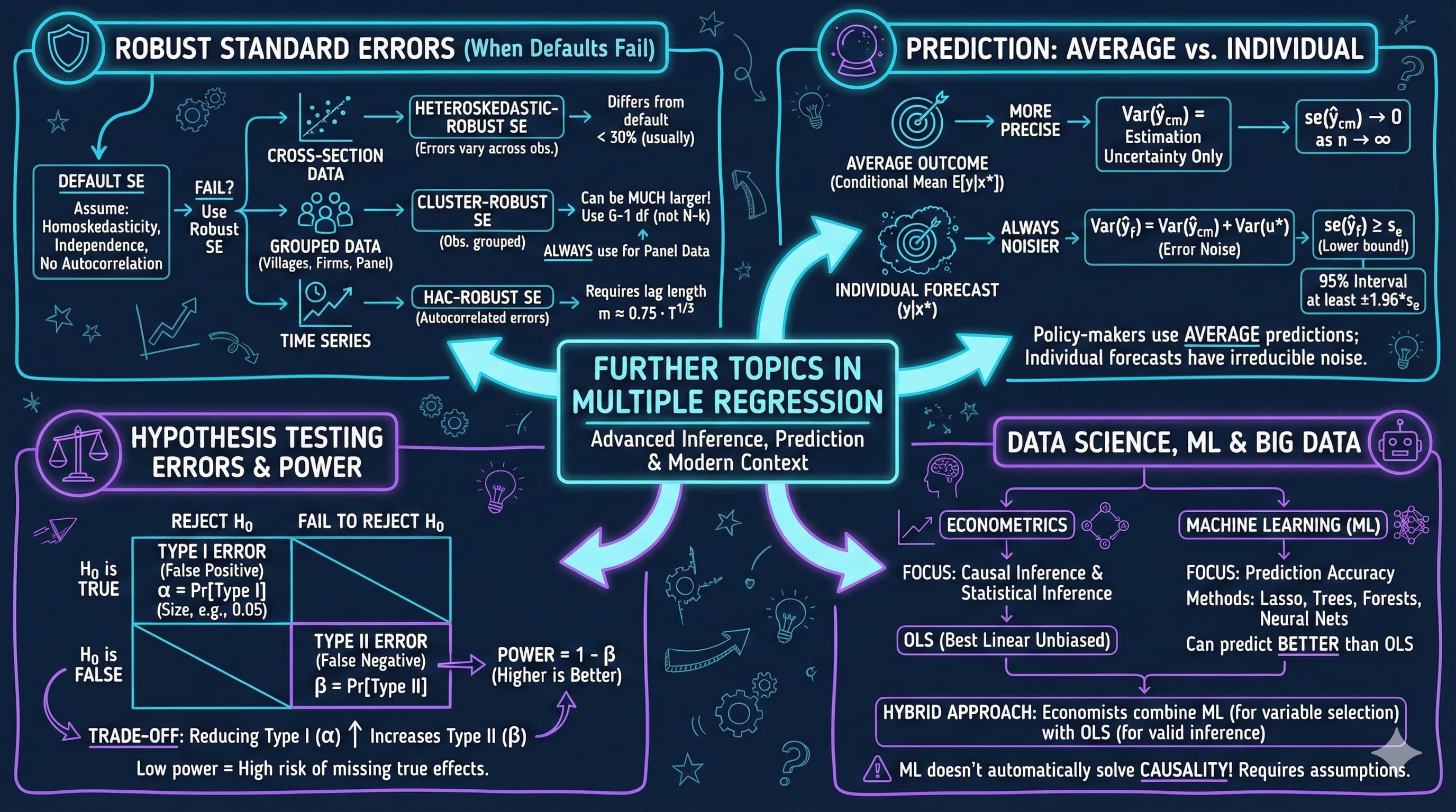
This chapter covers advanced topics that extend the multiple regression framework: robust standard errors for different data structures, prediction of outcomes, and deeper understanding of estimation and testing optimality.
**What you'll learn:**
- Understand when to use heteroskedastic-robust, cluster-robust, and HAC-robust standard errors
- Distinguish between prediction of average outcomes and individual outcomes
- Compute prediction intervals for conditional means and forecasts
- Understand the impact of nonrepresentative samples on regression estimates
- Recognize the difference between unbiased and best (most efficient) estimators
- Understand Type I and Type II errors in hypothesis testing
- Appreciate the role of bootstrap methods as an alternative to classical inference
- Know when OLS with robust SEs is preferred over more efficient estimators like FGLS
**Datasets used:**
- **AED_HOUSE.DTA**: 29 houses sold in Davis, California (1999) — for robust SEs and prediction
- **AED_REALGDPPC.DTA**: Real GDP per capita growth (241 observations) — for HAC standard errors
**Key economic questions:**
- Do conclusions about house prices change with robust standard errors?
- How precisely can we predict an individual house's price vs. the average price?
- What happens to inference when our sample is not representative?
**Chapter outline:**
- 12.1 Example - House Price Prediction
- 12.2 Inference with Robust Standard Errors
- 12.3 Prediction
- 12.4 Nonrepresentative Samples
- 12.5 Best Estimation Methods
- 12.6 Best Confidence Intervals
- 12.7 Best Tests
- Key Takeaways
- Practice Exercises
- Case Studies
## Key Concepts
Six core ideas anchor this chapter. Skim them before you start, and come back when a term feels fuzzy. Each entry pairs a concrete example using the chapter's data with a non-technical analogy. Click a panel to expand it.
**Cluster-Robust Standard Error:** A variant of robust standard errors that allows errors to be correlated *within* groups (clusters) but independent *across* them. It is the right correction when the data come in natural clusters — students in classrooms, workers in firms, municipalities in regions — because heteroskedasticity-only SEs (HC1) understate uncertainty in those settings.
::::: {.columns}
:::: {.column width="50%"}
::: {.callout-tip collapse="true" appearance="simple" title="Example"}
The Davis-house regression on `size`, `bedrooms`, `bathrooms`, `lotsize`, `age`, `monthsold` is fit with HC1 robust SEs because the 29 houses are an i.i.d. cross-section. If instead the data were 29 houses spread across a handful of *neighbourhoods*, errors within a neighbourhood would likely be correlated (shared school district, common buyer pool), and a cluster-robust SE keyed on neighbourhood would replace HC1 to keep inference honest.
:::
::::
:::: {.column width="50%"}
::: {.callout-note collapse="true" appearance="simple" title="Analogy"}
A school's test scores: students in the same classroom share a teacher, classroom climate, and rumor mill, so their scores aren't truly independent observations of "the population of students". Treating them as independent makes the school sound more confidently above-average than it is. Cluster-robust SEs let each *classroom* count as an effective unit of evidence — closer to the truth.
:::
::::
:::::
**Autocorrelation:** The phenomenon in time-series data of one period's error being correlated with the next period's error: $\operatorname{Corr}(u_t, u_{t-s}) \neq 0$. Positive autocorrelation means good periods (and bad periods) tend to cluster, so consecutive observations carry less independent information than a naive count suggests.
::::: {.columns}
:::: {.column width="50%"}
::: {.callout-tip collapse="true" appearance="simple" title="Example"}
For U.S. real-GDP-per-capita `growth` (`data_gdp`, $T = 241$ observations), the chapter computes a positive lag-1 autocorrelation — fast-growth years are more often followed by fast-growth years than chance would predict. That's why the Newey–West HAC standard error around the mean growth rate is *larger* than the default OLS SE: ignoring this serial dependence would overstate confidence.
:::
::::
:::: {.column width="50%"}
::: {.callout-note collapse="true" appearance="simple" title="Analogy"}
A handclap in a long stone hallway echoes for several seconds; sounds you make later overlap with the lingering echo from earlier. Autocorrelation is the data's echo — what happened a moment ago is still ringing, so today's reading isn't an independent observation of "the world", but partly a recording of yesterday's.
:::
::::
:::::
**Confidence Interval for the Conditional Mean ($E[Y \mid X^*]$):** A range covering, at a stated confidence level, the *average* value of $Y$ for a given $X^*$. Its standard error is $s_e \sqrt{1/n + (x^* - \bar{x})^2 / \sum(x_i - \bar{x})^2}$ in the bivariate case — both terms shrink to zero as $n \to \infty$.
::::: {.columns}
:::: {.column width="50%"}
::: {.callout-tip collapse="true" appearance="simple" title="Example"}
For a 2{,}000-sq-ft Davis house, the chapter's regression on `size` predicts an *average* `price` of about \$263k, with a 95% CI roughly $[\$253\mathrm{k}, \$272\mathrm{k}]$. That interval describes the typical sale price across all 2{,}000-sq-ft houses in this market — not what any single house will fetch.
:::
::::
:::: {.column width="50%"}
::: {.callout-note collapse="true" appearance="simple" title="Analogy"}
A bakery weighs every loaf and reports an average of 503 g. The CI for the *average* loaf is tight — say 501–505 g — because the bakery has weighed thousands. That number doesn't tell you how heavy *your* loaf is; it tells you what the bakery's process averages to across all customers.
:::
::::
:::::
**Prediction Interval for an Individual Outcome:** A range covering, at a stated confidence level, *the actual value* of $Y$ at a given $X^*$, including both estimation uncertainty and the irreducible noise $u^*$. The "$1 +$" in the formula $s_e \sqrt{1 + 1/n + (x^* - \bar{x})^2 / \sum(x_i - \bar{x})^2}$ never disappears — the floor on individual predictions is roughly $s_e$, no matter how large the sample.
::::: {.columns}
:::: {.column width="50%"}
::: {.callout-tip collapse="true" appearance="simple" title="Example"}
For the same 2{,}000-sq-ft house, the prediction interval for *one specific* sale is roughly $[\$213\mathrm{k}, \$312\mathrm{k}]$ — about five times wider than the CI for the average. With $s_e \approx \$23{,}551$ in the simple regression on `size`, almost all of that width comes from the irreducible "1" term, not from estimation uncertainty in $\hat\beta$.
:::
::::
:::: {.column width="50%"}
::: {.callout-note collapse="true" appearance="simple" title="Analogy"}
A casino slot machine has a known long-run payout of 95 cents on the dollar. That's the *conditional mean* — across thousands of pulls, you'll lose about 5%. For *your next pull*, though, you might win \$10 or lose \$1 — pure individual variation that the long-run average doesn't predict. The prediction interval is the range in which one pull will plausibly land.
:::
::::
:::::
**Generalized Least Squares (GLS):** A weighted-OLS estimator that re-weights observations by the inverse of their (assumed-known) error variances, restoring efficiency when the homoskedasticity assumption fails. In practice the variances are estimated from the data, yielding *feasible* GLS (FGLS) — but with risks: a misspecified weighting model can be worse than plain OLS with robust SEs.
::::: {.columns}
:::: {.column width="50%"}
::: {.callout-tip collapse="true" appearance="simple" title="Example"}
On the Davis house data, plain OLS yields the same $\hat\beta$ regardless of error structure — but its *efficiency* is lost under heteroskedasticity. A GLS estimator that down-weights houses with larger fitted-residual variance would, in principle, deliver tighter standard errors than OLS+HC1 — provided the weights are correctly specified. The chapter notes this trade-off and recommends OLS+robust SEs as the safe default.
:::
::::
:::: {.column width="50%"}
::: {.callout-note collapse="true" appearance="simple" title="Analogy"}
A tailor making suits doesn't apply the same fabric tension to every customer — a precise pattern weights tighter where measurements are reliable and looser where they are not. GLS is the regression's tailored fit: weighting each observation by its relative reliability so the resulting estimator hugs the truth more snugly than the off-the-rack OLS line does.
:::
::::
:::::
**Statistical Power ($1 - \beta$):** The probability that a test correctly *rejects* the null hypothesis when the alternative is in fact true. Power rises with sample size $n$, with the true effect size, and with the chosen significance level $\alpha$ — and falls with the noise level. A standard target is power $\geq 0.80$ for the smallest effect of practical interest.
::::: {.columns}
:::: {.column width="50%"}
::: {.callout-tip collapse="true" appearance="simple" title="Example"}
The Davis house regression had only $n = 29$ observations to test $H_0: \beta_{\text{bedrooms}} = 0$, and failed to reject ($p = 0.773$). With such a small sample and substantial multicollinearity between `size` and `bedrooms`, the test's power to detect a modest bedrooms effect was very low — the failure to reject is as likely a Type II error (missed effect) as evidence of no effect at all.
:::
::::
:::: {.column width="50%"}
::: {.callout-note collapse="true" appearance="simple" title="Analogy"}
A microscope's magnification determines whether a faint cell wall shows up or stays hidden in the smudge. Statistical power is the magnification of a hypothesis test: with low magnification, real effects can sit invisibly under the noise floor; bumping up the sample size is like swapping in a stronger lens — what was always there finally becomes visible.
:::
::::
:::::
## Setup
First, we import the necessary Python packages and configure the environment for reproducibility. All data will stream directly from GitHub.
```{python}
#| code-fold: true
#| code-summary: "Setup: Import libraries and configure environment"
# Import required packages
import numpy as np
import pandas as pd
import matplotlib.pyplot as plt
import seaborn as sns
import pyfixest as pf                     # fast estimation with robust SEs
from scipy import stats
from statsmodels.graphics.tsaplots import plot_acf
from statsmodels.tsa.stattools import acf
import random
import os

# Set random seeds for reproducibility
RANDOM_SEED = 42
random.seed(RANDOM_SEED)
np.random.seed(RANDOM_SEED)
os.environ['PYTHONHASHSEED'] = str(RANDOM_SEED)

# GitHub data URL
GITHUB_DATA_URL = "https://raw.githubusercontent.com/quarcs-lab/data-open/master/AED/"

# Set plotting style (dark theme matching book design)
plt.style.use('dark_background')
sns.set_style("darkgrid")
plt.rcParams.update({
    'axes.facecolor': '#1a2235',
    'figure.facecolor': '#12162c',
    'grid.color': '#3a4a6b',
    'figure.figsize': (10, 6),
    'text.color': 'white',
    'axes.labelcolor': 'white',
    'xtick.color': 'white',
    'ytick.color': 'white',
    'axes.edgecolor': '#1a2235',
})

print("Setup complete! Ready to explore further topics in multiple regression.")
```
## 12.1 Example - House Price Prediction
We'll work with two datasets:
1. **House price data** for cross-sectional robust inference
2. **GDP growth data** for time series HAC inference
```{python}
# 12.1 EXAMPLE - HOUSE PRICE PREDICTION

# Read house data
data_house = pd.read_stata(GITHUB_DATA_URL + 'AED_HOUSE.DTA')

print("House Data Summary:")
print(data_house.describe())

print("\nFirst few observations:")
data_house[['price', 'size', 'bedrooms', 'bathrooms', 'lotsize', 'age', 'monthsold']].head()
```
The dataset is a small cross-section: 29 houses sold in Davis, California, in 1999. Keep this in mind throughout the chapter — with only $n = 29$ observations, every standard-error comparison and hypothesis test operates with limited power.
## 12.2 Inference with Robust Standard Errors
In practice, the classical assumptions often fail. The most common violations are:
**1. Heteroskedasticity**: Error variance varies across observations
- Common in cross-sectional data
- Makes default standard errors incorrect
- Solution: Use **heteroskedasticity-robust standard errors** (HC1, White's correction)
**2. Clustered errors**: Errors correlated within groups
- Common in panel data, hierarchical data
- Makes default and het-robust SEs too small
- Solution: Use **cluster-robust standard errors**
**3. Autocorrelation**: Errors correlated over time
- Common in time series
- Makes default SEs incorrect
- Solution: Use **HAC (Newey-West) standard errors**
**Key insight**: OLS coefficients remain unbiased under these violations, but standard errors need adjustment.
**Heteroskedastic-robust standard error formula**:
$$se_{het}(\hat{\beta}_j) = \sqrt{\frac{\sum_{i=1}^n \tilde{x}_{ji}^2 \hat{u}_i^2}{(\sum_{i=1}^n \tilde{x}_{ji}^2)^2}}$$
where $\tilde{x}_{ji}$ are residuals from regressing $x_j$ on other regressors, and $\hat{u}_i$ are OLS residuals.
```{python}
# 12.2 INFERENCE WITH ROBUST STANDARD ERRORS

# Estimate with default standard errors
model_default = pf.feols('price ~ size + bedrooms + bathrooms + lotsize + age + monthsold', data=data_house)

# Key results
size_coef_default = model_default.coef()['size']
size_pval_default = model_default.pvalue()['size']
r_squared = model_default._r2
print(f"Size effect (default): ${size_coef_default:,.2f} per sq ft (p = {size_pval_default:.4f})")
print(f"R-squared: {r_squared:.4f}")

# Full regression output
print("\nRegression with Default Standard Errors:")
model_default.summary()
```
Now we re-estimate the identical model with heteroskedastic-robust (HC1) standard errors. The coefficient estimates will not change — watch instead how each standard error, $t$-statistic, and $p$-value shifts relative to the default output above.
```{python}
# Estimate with heteroskedastic-robust standard errors (HC1)
model_robust = pf.feols('price ~ size + bedrooms + bathrooms + lotsize + age + monthsold', data=data_house, vcov='HC1')

# Key results
size_coef_robust = model_robust.coef()['size']
size_pval_robust = model_robust.pvalue()['size']
print(f"Size effect (robust): ${size_coef_robust:,.2f} per sq ft (p = {size_pval_robust:.4f})")

# Full regression output
print("\nRegression with Heteroskedastic-Robust Standard Errors (HC1):")
model_robust.summary()
```
For the Davis houses, robust and default standard errors tell the same story: the robust SE for `size` (15.36) is nearly identical to the default (15.39), so the headline conclusion is unchanged — each additional square foot is associated with roughly \$68 more in sale price, highly significant either way (p = 0.0002). The largest adjustments are for `bathrooms` (robust SE about 23% larger) and `lotsize` (robust SE about 26% smaller), but both variables remain far from statistical significance under either method.
> **Key Concept 12.1: Heteroskedastic-Robust Standard Errors**
>
> When error variance is not constant across observations, default OLS standard errors are invalid. Heteroskedastic-robust (HC1) SEs correct this problem without changing the coefficient estimates themselves. Only the standard errors, $t$-statistics, and confidence intervals change. For cross-sectional data, reporting HC1 robust SEs is considered best practice.
### Comparison: Default vs. Robust Standard Errors
Let's systematically compare the standard errors and see how inference changes.
```{python}
# Compare default vs. robust (HC1) standard errors, coefficient by coefficient
print(f"{'Variable':<14} {'Coef':>12} {'Default SE':>12} {'Robust SE':>12} {'SE Ratio':>10}")
print("-" * 62)
for var in model_default.coef().index:
    coef  = model_default.coef()[var]
    se_d  = model_default.se()[var]
    se_r  = model_robust.se()[var]
    ratio = se_r / se_d                    # ratio > 1 -> default SE was too optimistic
    print(f"{var:<14} {coef:>12.2f} {se_d:>12.2f} {se_r:>12.2f} {ratio:>10.3f}")
```
### Interpreting the Comparison: What Changed?
**Understanding the Results:**
Looking at the SE Ratio column, we can see how robust standard errors differ from default ones:
**When SE Ratio > 1.0**: Robust SE is larger than default SE
- Suggests heteroskedasticity is present
- Default SEs were **understating** uncertainty
- t-statistics decrease, p-values increase
- We were **too confident** in rejecting null hypotheses
**When SE Ratio ≈ 1.0**: Robust SE similar to default SE
- Little evidence of heteroskedasticity for this variable
- Both methods give similar inference
**When SE Ratio < 1.0**: Robust SE smaller than default SE
- Unusual but possible
- Could indicate negative correlation between x² and squared residuals
**Practical Implications:**
1. **Coefficient estimates unchanged**: OLS point estimates are the same regardless of SE type
2. **Inference changes**: Variables significant with default SEs might become insignificant with robust SEs
3. **Publication standard**: Most journals now require robust SEs for cross-sectional data
4. **Conservative approach**: When in doubt, report robust SEs (they're generally more credible)
**Rule of thumb**: If robust SEs differ substantially (>30% change), heteroskedasticity is likely present and you should use robust inference.
### HAC Standard Errors for Time Series
Time series data often exhibit **autocorrelation**: current errors correlated with past errors.
**Example**: GDP growth tends to persist
- Positive shock today → likely positive next period
- Creates correlation structure $Corr(u_t, u_{t-s}) \neq 0$
**HAC (Newey-West) standard errors**:
- Account for both heteroskedasticity AND autocorrelation
- Require specifying maximum lag length $m$
- Rule of thumb: $m = 0.75 \times T^{1/3}$
**Autocorrelation function**:
$$\rho_s = \frac{Cov(y_t, y_{t-s})}{\sqrt{Var(y_t) Var(y_{t-s})}}$$
We can visualize this with a **correlogram**.
```{python}
# Load GDP growth data
data_gdp = pd.read_stata(GITHUB_DATA_URL + 'AED_REALGDPPC.DTA')

# HAC Standard Errors for Time Series Data

print("\nGDP Growth Data Summary:")
print(data_gdp['growth'].describe())

# Mean of growth
mean_growth = data_gdp['growth'].mean()
print(f"\nMean growth rate: {mean_growth:.6f}")
```
Before adjusting any standard errors, let's measure the serial dependence directly. The next cell computes the autocorrelation of `growth` at lags 0 through 5 — look for a positive lag-1 value, which means one period's growth carries information about the next.
```{python}
# Autocorrelation analysis
print("\nAutocorrelations at multiple lags:")
acf_values = acf(data_gdp['growth'].dropna(), nlags=5, fft=False)
for i in range(6):
    print(f"  Lag {i}: {acf_values[i]:.6f}")

# Positive lag 1 correlation suggests persistence
```
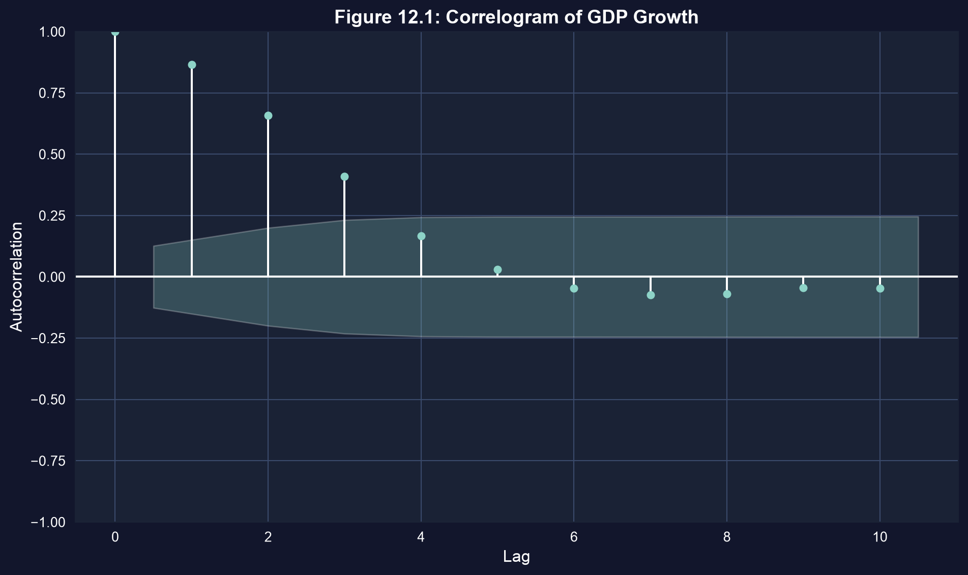
Now we plot the correlogram (Figure 12.1), which displays the autocorrelation at each lag together with 95% confidence bands under the null of no autocorrelation.
```{python}
# Correlogram
fig, ax = plt.subplots(figsize=(10, 6))
plot_acf(data_gdp['growth'].dropna(), lags=10, ax=ax, alpha=0.05)
ax.set_xlabel('Lag', fontsize=12)
ax.set_ylabel('Autocorrelation', fontsize=12)
ax.set_title('Figure 12.1: Correlogram of GDP Growth', fontsize=14, fontweight='bold')
plt.tight_layout()
plt.show()

print("The correlogram shows autocorrelation at various lags.")
print("Blue shaded area = 95% confidence bands under null of no autocorrelation.")
```
**What to look for in this correlogram:**
- **Bars outside the shaded band**: Autocorrelations that exceed the 95% confidence bands are statistically significant, indicating persistent serial correlation
- **Decay pattern**: Autocorrelations that decay slowly suggest strong persistence in the series; rapid decay suggests shocks are short-lived
- **Lag 1 autocorrelation**: The most important lag -- a large positive value means today's growth predicts tomorrow's growth
> **Key Concept 12.2: HAC Standard Errors for Time Series**
>
> In time series data, errors are often autocorrelated — today's shock persists into tomorrow. HAC (heteroskedasticity and autocorrelation consistent) standard errors, also called Newey-West SEs, account for both heteroskedasticity and autocorrelation. The lag length $m$ must be specified; a common rule of thumb is $m = 0.75 \times T^{1/3}$.
Now let's compute the standard error of the mean growth rate three ways: the default SE (which assumes independence), a HAC SE at lag 0 (heteroskedasticity-robust only), and a HAC SE at the rule-of-thumb lag (Newey-West), which also corrects for autocorrelation.
```{python}
# HAC (Newey-West) standard errors for the mean growth rate
from statsmodels.regression.linear_model import OLS as smOLS

growth   = data_gdp['growth'].dropna()      # drop initial missing growth values
n_gdp    = len(growth)
lag_rule = int(0.75 * n_gdp**(1/3))         # rule of thumb: m = 0.75 x T^(1/3)

# Default SE assumes no autocorrelation
se_default = growth.std() / np.sqrt(n_gdp)

# HAC SEs via an intercept-only OLS (the mean model)
y = growth
X = np.ones(n_gdp)
se_hac0 = smOLS(y, X).fit(cov_type='HAC', cov_kwds={'maxlags': 0}).bse.iloc[0]
se_hac  = smOLS(y, X).fit(cov_type='HAC', cov_kwds={'maxlags': lag_rule}).bse.iloc[0]

print(f"Mean growth rate: {growth.mean():.4f}  (T = {n_gdp})")
print(f"Default SE (no autocorrelation):   {se_default:.6f}")
print(f"HAC SE (lag 0, het-robust only):   {se_hac0:.6f}")
print(f"HAC SE (lag {lag_rule}, Newey-West):         {se_hac:.6f}")
print(f"Ratio HAC(lag {lag_rule}) / Default: {se_hac / se_default:.3f}")
```
### Interpreting HAC Standard Errors
**What the Results Tell Us:**
Comparing the three standard error estimates for the mean growth rate:
1. **Default SE** (assumes no autocorrelation):
- Smallest standard error
- Assumes errors are independent over time
- **Underestimates** uncertainty when autocorrelation exists
2. **HAC with lag 0** (het-robust only):
- Accounts for heteroskedasticity but not autocorrelation
- Often similar to default in time series
- Still underestimates uncertainty if autocorrelation present
3. **HAC with lag 4** (Newey-West):
- Accounts for both heteroskedasticity AND autocorrelation
- **Larger SE** reflects true uncertainty
- More conservative but valid inference
**Why is HAC SE larger?**
Autocorrelation creates **information overlap** between observations:
- If growth today predicts growth tomorrow, consecutive observations aren't fully independent
- We have **less effective information** than the sample size suggests
- Standard errors must increase to reflect this
**Practical guidance:**
- For time series data, **always use HAC SEs**
- Lag length choice: Rule of thumb = 0.75 × T^(1/3)
- For T=100: m ≈ 3-4 lags
- For T=200: m ≈ 4-5 lags
- Err on the side of more lags (inference remains valid)
- Check sensitivity to lag length
**The cost of ignoring autocorrelation:**
- Overconfident inference (SEs too small)
- Spurious significance (false discoveries)
- Invalid hypothesis tests
## 12.3 Prediction
Prediction is a core application of regression, but there's a crucial distinction:
**1. Predicting the conditional mean** $E[y | x^*]$
- Average outcome for given $x^*$
- More precise (smaller standard error)
- Used for policy analysis, average effects
**2. Predicting an actual value** $y | x^*$
- Individual outcome including random error
- Less precise (larger standard error)
- Used for forecasting individual cases
**Key formulas**:
Conditional mean:
$$E[y | x^*] = \beta_1 + \beta_2 x_2^* + \cdots + \beta_k x_k^*$$
Actual value:
$$y | x^* = \beta_1 + \beta_2 x_2^* + \cdots + \beta_k x_k^* + u^*$$
**Standard errors**:
For conditional mean (bivariate case):
$$se(\hat{y}_{cm}) = s_e \sqrt{\frac{1}{n} + \frac{(x^* - \bar{x})^2}{\sum(x_i - \bar{x})^2}}$$
For actual value (bivariate case):
$$se(\hat{y}_f) = s_e \sqrt{1 + \frac{1}{n} + \frac{(x^* - \bar{x})^2}{\sum(x_i - \bar{x})^2}}$$
Note the "1 +" term for actual values - this reflects the irreducible uncertainty from $u^*$.
```{python}
# 12.3 PREDICTION

# Simple regression: price on size
model_simple = pf.feols('price ~ size', data=data_house)

print("\nSimple regression: price = β₀ + β₁·size + u")
print(f"  β₀ (Intercept): ${model_simple.coef()['Intercept']:.2f}")
print(f"  β₁ (Size): ${model_simple.coef()['size']:.4f}")
print(f"  R²: {model_simple._r2:.4f}")
print(f"  Root MSE (σ̂): ${np.sqrt(np.sum(model_simple._u_hat**2) / (int(model_simple._N) - len(model_simple.coef()))):.2f}")
```
> **Key Concept 12.3: Predicting Conditional Means vs. Individual Outcomes**
>
> Predicting the average outcome $E[y|x^*]$ is more precise than predicting an individual $y|x^*$. The forecast variance equals the conditional mean variance plus $\text{Var}(u^*)$: $\text{Var}(\hat{y}_f) = \text{Var}(\hat{y}_{cm}) + \sigma^2$. As $n \to \infty$, the conditional mean SE shrinks to zero, but the forecast SE remains at least $s_e$ — a fundamental limit on individual predictions.
### Why Are Prediction Intervals So Much Wider?
**The Fundamental Difference:**
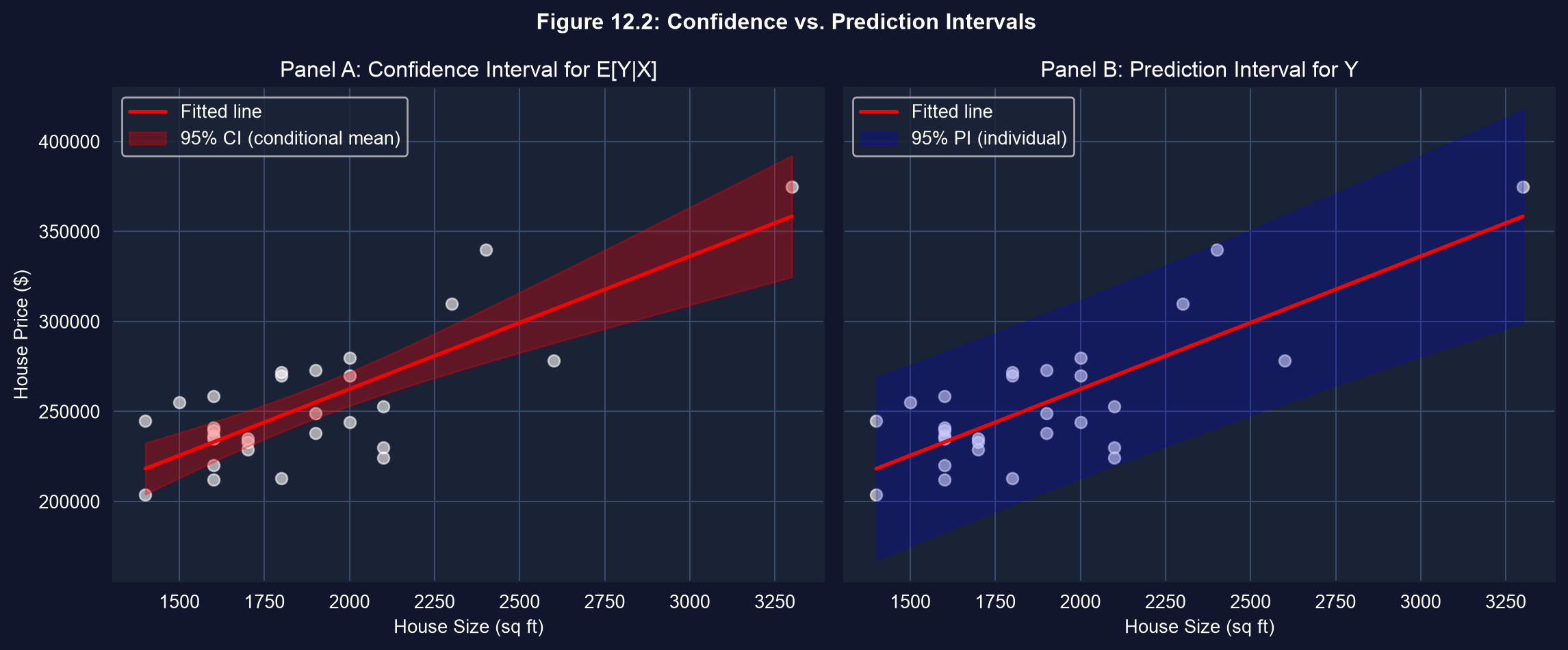
Looking at the two panels, you'll notice the **prediction interval (blue) is dramatically wider** than the confidence interval (red). This isn't a mistake—it reflects a fundamental distinction in what we're predicting.
**Confidence Interval for E[Y|X] (Red):**
- Predicts the **average** price for all 2000 sq ft houses
- Uncertainty comes only from **estimation error** in β̂
- As sample size increases (n → ∞), this interval **shrinks to zero**
- Formula includes: 1/n term (goes to 0 as n grows)
**Prediction Interval for Y (Blue):**
- Predicts an **individual** house price
- Uncertainty comes from:
1. **Estimation error** in β̂ (same as CI)
2. **Irreducible randomness** in the individual outcome (u*)
- Even with perfect knowledge of β, individual predictions remain uncertain
- Formula includes: **"1 +"** term (never goes away)
**Intuitive Example:**
Imagine predicting height from age:
- **Conditional mean**: Average height of all 10-year-olds = 140 cm
- We can estimate this average very precisely
- CI might be [139, 141] cm
- **Actual value**: A specific 10-year-old's height
- Could be anywhere from 120 to 160 cm
- PI might be [125, 155] cm
- Even knowing the average perfectly doesn't eliminate individual variation
**Mathematical Insight:**
$$se(\hat{y}_f) = \sqrt{s_e^2 + se(\hat{y}_{cm})^2}$$
- First term (s_e²): Irreducible error variance—dominates the formula
- Second term: Estimation uncertainty—becomes negligible with large samples
- Result: PI width ≈ 2 × 1.96 × s_e ≈ 4 × RMSE
**Practical Implications:**
1. **Don't confuse the two**: Predicting averages is much more precise than predicting individuals
2. **Policy vs. forecasting**:
- Policy analysis (average effects) → Use confidence intervals
- Individual forecasting (who will default?) → Use prediction intervals
3. **Communicating uncertainty**: Always show prediction intervals for individual forecasts
4. **Limits of prediction**: No amount of data eliminates individual-level uncertainty
### Visualization: Confidence vs. Prediction Intervals
This figure illustrates the fundamental difference between:
- **Confidence interval for conditional mean** (narrower, red)
- **Prediction interval for actual value** (wider, blue)
```{python}
# Figure 12.2: confidence interval (conditional mean) vs. prediction interval (individual)
sizes  = data_house['size'].values
xbar   = sizes.mean()
Sxx    = np.sum((sizes - xbar)**2)
n_h    = len(data_house)
s_e    = np.sqrt(np.sum(model_simple._u_hat**2) / (n_h - len(model_simple.coef())))
t_crit = stats.t.ppf(0.975, n_h - len(model_simple.coef()))

grid = pd.DataFrame({'size': np.linspace(sizes.min(), sizes.max(), 100)})
fit  = model_simple.predict(newdata=grid)
dist = (grid['size'].values - xbar)**2 / Sxx
se_cm_grid = s_e * np.sqrt(1/n_h + dist)          # conditional-mean SE
se_pi_grid = s_e * np.sqrt(1 + 1/n_h + dist)      # individual-forecast SE

fig, (ax1, ax2) = plt.subplots(1, 2, figsize=(12, 5), sharey=True)

# Panel A: confidence interval for the average price (red)
ax1.scatter(data_house['size'], data_house['price'], s=40, alpha=0.6, color='white')
ax1.plot(grid['size'], fit, color='red', linewidth=2, label='Fitted line')
ax1.fill_between(grid['size'], fit - t_crit*se_cm_grid, fit + t_crit*se_cm_grid,
                 color='red', alpha=0.30, label='95% CI (conditional mean)')
ax1.set_title('Panel A: Confidence Interval for E[Y|X]')
ax1.set_xlabel('House Size (sq ft)')
ax1.set_ylabel('House Price ($)')
ax1.legend()

# Panel B: prediction interval for one individual house (blue)
ax2.scatter(data_house['size'], data_house['price'], s=40, alpha=0.6, color='white')
ax2.plot(grid['size'], fit, color='red', linewidth=2, label='Fitted line')
ax2.fill_between(grid['size'], fit - t_crit*se_pi_grid, fit + t_crit*se_pi_grid,
                 color='blue', alpha=0.20, label='95% PI (individual)')
ax2.set_title('Panel B: Prediction Interval for Y')
ax2.set_xlabel('House Size (sq ft)')
ax2.legend()

fig.suptitle('Figure 12.2: Confidence vs. Prediction Intervals', fontweight='bold')
plt.tight_layout()
plt.show()
```
### Understanding the Numbers: A Concrete Example
**Interpreting the Results for a 2000 sq ft House:**
Looking at our predictions, several patterns emerge:
**1. Point Prediction:**
- Predicted price ≈ \$263,000 (approximately)
- This is our best single guess
- Same for both conditional mean and actual value
**2. Confidence Interval for E[Y|X=2000]:**
- Relatively narrow (e.g., \$253k - \$272k)
- Tells us: "We're 95% confident the **average price** of all 2000 sq ft houses is in this range"
- Precise because we're estimating a population average
- Useful for: Understanding market valuations, setting pricing policies
**3. Prediction Interval for Y:**
- Much wider (e.g., \$213k - \$312k)
- Tells us: "We're 95% confident **this specific house** will sell in this range"
- Wide because individual houses vary considerably
- Useful for: Setting listing ranges, individual appraisals
**The Ratio is Revealing:**
Notice that the PI is approximately **5 times wider** than the CI. This ratio tells us:
- Most variation is **between houses** (individual heterogeneity)
- Relatively little variation is **estimation uncertainty**
- Adding more data would shrink the CI but barely affect the PI
**Statistical vs. Economic Significance:**
- **CI width** = Statistical precision (how well we know β)
- **PI width** = Economic uncertainty (inherent market volatility)
- In this example: Good statistical precision, but still substantial economic uncertainty
**Practical Takeaway:**
If you're a real estate agent:
- Don't promise a precise price (\$263k)
- Do provide a realistic range (\$213k - \$312k)
- Explain that individual houses vary, even controlling for size
- Use the confidence interval to discuss average market values
### Deconstructing the Standard Error Formulas
**Understanding Where the "1 +" Comes From:**
The manual calculations reveal the mathematical structure of prediction uncertainty:
**For Conditional Mean:**
$$se(\hat{y}_{cm}) = \hat{\sigma} \sqrt{\frac{1}{n} + \frac{(x^* - \bar{x})^2}{\sum(x_i - \bar{x})^2}}$$
- **First term (1/n)**: Decreases with sample size—more data reduces uncertainty
- **Second term**: Distance from mean matters—extrapolation is risky
- Prediction at $x^* = \bar{x}$ (sample mean) is most precise
- Prediction far from $\bar{x}$ is less precise
- Both terms → 0 as n → ∞ (perfect knowledge of E[Y|X])
**For Actual Value:**
$$se(\hat{y}_f) = \hat{\sigma} \sqrt{1 + \frac{1}{n} + \frac{(x^* - \bar{x})^2}{\sum(x_i - \bar{x})^2}}$$
- **The critical "1 +"**: Represents $Var[u^*]$, the future error term
- This term **never disappears**, even with infinite data
- Dominates the formula in moderate to large samples
**Numerical Insight:**
In our example:
- $\hat{\sigma}$ (RMSE) ≈ \$23.6k (this is the irreducible uncertainty)
- $(1/n)$ term ≈ 0.034 (small with n=29)
- Distance term varies with prediction point
For predictions near the mean:
- $se(\hat{y}_{cm})$ ≈ \$23.6k × √0.034 ≈ \$4.4k (mainly from 1/n)
- $se(\hat{y}_f)$ ≈ \$23.6k × √1.034 ≈ \$24k (mainly from the "1")
**The "1 +" term is why:**
- Prediction intervals don't shrink much with more data
- Individual predictions remain uncertain even with perfect models
- $se(\hat{y}_f) \approx \hat{\sigma}$ in large samples
**Geometric Interpretation:**
The funnel shape in prediction plots comes from the distance term:
- Narrow near $\bar{x}$ (center of data)
- Wider at extremes (extrapolation region)
- But even at the center, PI is wide due to the "1" term
**Practical Lesson:**
When presenting predictions:
1. Always acknowledge the "1 +" uncertainty
2. Be most confident about predictions near the data center
3. Be especially cautious about extrapolation (predictions outside the data range)
4. Understand that better models reduce estimation error but not irreducible randomness
### Prediction at Specific Values
Let's predict house price for a 2000 square foot house.
```{python}
# Prediction at a specific value: a 2000 sq ft house (simple regression on size)
x_star  = 2000
pred_cm = model_simple.predict(newdata=pd.DataFrame({'size': [x_star]}))[0]

# Ingredients for the bivariate prediction standard errors
sizes  = data_house['size'].values
xbar   = sizes.mean()
Sxx    = np.sum((sizes - xbar)**2)
n_h    = len(data_house)
s_e    = np.sqrt(np.sum(model_simple._u_hat**2) / (n_h - len(model_simple.coef())))
t_crit = stats.t.ppf(0.975, n_h - len(model_simple.coef()))

se_cm = s_e * np.sqrt(1/n_h + (x_star - xbar)**2 / Sxx)      # conditional-mean SE
se_pi = s_e * np.sqrt(1 + 1/n_h + (x_star - xbar)**2 / Sxx)  # individual-forecast SE

ci_low, ci_high = pred_cm - t_crit*se_cm, pred_cm + t_crit*se_cm
pi_low, pi_high = pred_cm - t_crit*se_pi, pred_cm + t_crit*se_pi

print(f"Prediction for a {x_star:,} sq ft house (simple regression on size):")
print(f"  Point prediction:              ${pred_cm:,.0f}")
print(f"  95% CI for the average price:  [${ci_low:,.0f}, ${ci_high:,.0f}]")
print(f"  95% PI for one specific house: [${pi_low:,.0f}, ${pi_high:,.0f}]")
print(f"  PI width / CI width:           {(pi_high - pi_low) / (ci_high - ci_low):.2f}x")
```
### Manual Calculation of Standard Errors
Let's manually calculate the standard errors to understand the formulas.
```{python}
# Manual decomposition of the prediction standard errors at x* = 2000
print("Standard-error ingredients at x* = 2000 sq ft:")
print(f"  s_e (RMSE):                        ${s_e:,.0f}")
print(f"  1/n term:                          {1/n_h:.4f}")
print(f"  distance term (x*-xbar)^2 / Sxx:   {(x_star - xbar)**2 / Sxx:.4f}")
print(f"  se(y_cm) = s_e * sqrt(1/n + dist)      = ${se_cm:,.0f}")
print(f"  se(y_f)  = s_e * sqrt(1 + 1/n + dist)  = ${se_pi:,.0f}")
print(f"\nThe '1 +' term dominates: se(y_f) is about {se_pi/se_cm:.1f}x larger than se(y_cm).")
```
### Prediction with Multiple Regression
Now let's predict using the full multiple regression model.
```{python}
# Prediction for Multiple Regression

model_multi = pf.feols('price ~ size + bedrooms + bathrooms + lotsize + age + monthsold', data=data_house)

# Predict for specific values
new_house = pd.DataFrame({
    'size': [2000],
    'bedrooms': [4],
    'bathrooms': [2],
    'lotsize': [2],
    'age': [40],
    'monthsold': [6]
})

# Predict using pyfixest
pred_value = model_multi.predict(newdata=new_house)[0]

print("\nPrediction for:")
print("  size=2000, bedrooms=4, bathrooms=2, lotsize=2, age=40, monthsold=6")
print(f"\nPredicted price: ${pred_value:.2f}")

# Prediction interval for actual value (manual computation)
n_multi = len(data_house)
k_multi = len(model_multi.coef())
s_e_multi = np.sqrt(np.sum(model_multi._u_hat**2) / (n_multi - k_multi))
tcrit_multi = stats.t.ppf(0.975, n_multi - k_multi)

# Approximate prediction interval (using RMSE as dominant term)
pi_lower = pred_value - tcrit_multi * s_e_multi
pi_upper = pred_value + tcrit_multi * s_e_multi

print(f"\n95% PI for Y (approximate):")
print(f"  [${pi_lower:.2f}, ${pi_upper:.2f}]")
print(f"  RMSE: ${s_e_multi:.2f}")

print("\nNote: adding regressors does not automatically improve precision —")
print("here the RMSE is slightly larger than in the simple regression.")
print("Individual predictions still have large uncertainty.")
```
### Prediction with Robust Standard Errors
When heteroskedasticity is present, we should use robust standard errors for prediction intervals too.
```{python}
# Prediction with Heteroskedastic-Robust SEs

model_multi_robust = pf.feols('price ~ size + bedrooms + bathrooms + lotsize + age + monthsold', data=data_house, vcov='HC1')

# Predict using pyfixest with robust SEs
pred_robust_value = model_multi_robust.predict(newdata=new_house)[0]

print(f"\nPredicted price: ${pred_robust_value:.2f}")

# Robust prediction interval (approximate)
s_e_robust = np.sqrt(np.sum(model_multi_robust._u_hat**2) / (n_multi - k_multi))
pi_lower_robust = pred_robust_value - tcrit_multi * s_e_robust
pi_upper_robust = pred_robust_value + tcrit_multi * s_e_robust

print(f"\nRobust 95% PI for Y (approximate):")
print(f"  [${pi_lower_robust:.2f}, ${pi_upper_robust:.2f}]")
print(f"  RMSE: ${s_e_robust:.2f}")

print("\nComparison of default vs. robust predictions:")
print(f"  RMSE (default): ${s_e_multi:.2f}")
print(f"  RMSE (robust): ${s_e_robust:.2f}")
print(f"  Note: Coefficients and RMSE are identical; only SEs for inference differ.")
```
> **Key Concept 12.4: Why Individual Forecasts Are Imprecise**
>
> Even with precisely estimated coefficients, predicting an individual outcome is imprecise because the forecast must account for the unobservable error $u^*$. The forecast standard error satisfies $se(\hat{y}_f) \geq s_e$ — it is at least as large as the regression's standard error. This means 95% prediction intervals are at least $\pm 1.96 \times s_e$ wide, regardless of how much data we have.
## 12.4 Nonrepresentative Samples
**Sample selection** can bias OLS estimates:
**Case 1: Selection on regressors** (X)
- Example: Oversample high-income households
- OLS remains unbiased if we include income as a control
- Solution: Include selection variables as controls
**Case 2: Selection on outcome** (Y)
- Example: Survey excludes very high earners
- OLS estimates are biased for population parameters
- Solution: Sample weights, Heckman correction, or other selection models
**Survey weights**:
- Many surveys provide weights to adjust for nonrepresentativeness
- Use **weighted least squares (WLS)** instead of OLS
- Weight formula: $w_i = 1 / P(\text{selected})$
**Key insight**: Always check whether your sample is representative of your target population!
### Bootstrap Confidence Intervals: An Alternative Approach
**What is Bootstrap?**
The bootstrap is a computational method that:
1. **Resamples** your data many times (e.g., 1000 replications)
2. **Re-estimates** the model for each resample
3. Uses the **distribution of estimates** to build confidence intervals
**How it works:**
For each bootstrap replication b = 1, ..., B:
1. Draw n observations **with replacement** from original data
2. Estimate regression: $\hat{\beta}_j^{(b)}$
3. Store the coefficient estimate
After B replications:
- You have B estimates: $\{\hat{\beta}_j^{(1)}, \hat{\beta}_j^{(2)}, ..., \hat{\beta}_j^{(B)}\}$
- These form an empirical distribution
**Percentile Method CI:**
- 95% CI = [2.5th percentile, 97.5th percentile] of bootstrap distribution
- Example: If you have 1000 estimates, use the 25th and 975th values after sorting from smallest to largest
**Advantages of Bootstrap:**
1. **No distributional assumptions**: Don't need to assume normality
2. **Works for complex statistics**: Medians, ratios, quantiles, etc.
3. **Better small-sample coverage**: Often more accurate than asymptotic formulas
4. **Flexibility**: Can bootstrap residuals, observations, or both
5. **Visual understanding**: See the actual sampling distribution
**When to use Bootstrap:**
- Small samples (n < 30-50)
- Non-standard statistics (beyond means and coefficients)
- Skewed or heavy-tailed distributions
- Checking robustness of standard inference
- When asymptotic formulas are complex or unavailable
**Limitations:**
- Computationally intensive (need B = 1000+ replications)
- Requires careful implementation (stratification, cluster bootstrap)
- May fail with very small samples (n < 10)
- Assumes sample is representative of population
**Bootstrap vs. Robust SEs:**
Both address uncertainty, but differently:
- **Robust SEs**: Analytical correction for heteroskedasticity/autocorrelation
- **Bootstrap**: Computational approach using resampling
Often used together: Bootstrap with robust methods!
**Practical Implementation Tips:**
1. Use B ≥ 1000 for confidence intervals
2. Set random seed for reproducibility
3. For time series: Use block bootstrap (resample blocks, not individuals)
4. For panel data: Use cluster bootstrap (resample clusters)
5. Check convergence: Results shouldn't change much with different seeds
```{python}
# 12.4 NONREPRESENTATIVE SAMPLES — key insight

print("Sample selection and OLS bias:\n")
print("- Selection on X (a regressor): OLS stays unbiased if X is controlled")
print("  for; it only costs precision.")
print("- Selection on Y (the outcome): OLS is biased for population parameters")
print("  -- use sample weights, a Heckman correction, or a selection model.")
print("\nAlways verify your sample is representative of the target population.")
```
> **Key Concept 12.5: Sample Selection Bias**
>
> If the sample is not representative of the population, OLS estimates may be biased. Selection on the dependent variable $Y$ (e.g., studying only high earners) is particularly problematic. Selection on the regressors $X$ (e.g., studying only college graduates) is less harmful because it reduces precision but doesn't necessarily bias coefficient estimates.
### The Type I vs. Type II Error Tradeoff
**Understanding the Table:**
The 2×2 decision table reveals a fundamental tradeoff in hypothesis testing:
| Decision | H₀ True | H₀ False |
|----------|---------|----------|
| Reject H₀ | **Type I error (α)** | **Correct (Power)** |
| Don't reject | Correct (1-α) | **Type II error (β)** |
**Type I Error (False Positive):**
- Reject a true null hypothesis
- Probability = significance level α (we control this)
- Example: Conclude a drug works when it doesn't
- **"Seeing patterns in noise"**
**Type II Error (False Negative):**
- Fail to reject a false null hypothesis
- Probability = β (harder to control)
- Example: Miss a real drug effect
- **"Missing real signals"**
**The Fundamental Tradeoff:**
If we make the test **stricter** (lower α):
- Fewer false positives (Type I errors)
- More false negatives (Type II errors)
- Lower power (harder to detect real effects)
If we make the test **looser** (higher α):
- Higher power (easier to detect real effects)
- More false positives (Type I errors)
**Statistical Power = 1 - β:**
- Probability of correctly rejecting false H₀
- "Sensitivity" of the test
- Want power ≥ 0.80 (80% chance of detecting real effect)
**What Affects Power?**
1. **Sample size (n)**: Larger n → Higher power
2. **Effect size (β)**: Larger true effect → Higher power
3. **Significance level (α)**: Higher α → Higher power (but more Type I errors)
4. **Noise level (σ)**: Lower σ → Higher power
**The Power Function:**
Power depends on the **true parameter value**:
- At β = 0 (H₀ true): Power = α (just Type I error rate)
- As |β| increases: Power increases
- For very large |β|: Power → 1 (almost certain detection)
**Multiple Testing Problem:**
Testing k hypotheses at α = 0.05:
- Expected false positives = 0.05 × k
- Test 20 hypotheses → expect 1 false positive even if all H₀ are true!
**Solutions:**
1. **Bonferroni correction**: Use α/k for each test (conservative)
2. **False Discovery Rate (FDR)**: Control proportion of false positives
3. **Pre-registration**: Specify primary hypotheses before seeing data
4. **Replication**: Confirm findings in independent samples
## 12.5 Best Estimation Methods
**When are OLS estimators "best"?**
Under classical assumptions 1-4, OLS is **BLUE** (Best Linear Unbiased Estimator) by the Gauss-Markov Theorem.
**When assumptions fail:**
**1. Heteroskedasticity**: $Var[u_i | X] = \sigma_i^2$ (varies)
- OLS remains unbiased but inefficient
- **Feasible GLS (FGLS)** or **Weighted Least Squares (WLS)** more efficient
- Weight observations inversely to error variance: $w_i = 1/\sigma_i^2$
**2. Autocorrelation**: $Cov[u_t, u_{t-s}] \neq 0$
- OLS remains unbiased but inefficient
- **FGLS with AR errors** more efficient
- Model error structure: $u_t = \rho u_{t-1} + \epsilon_t$
**Practical advice**:
- Most applied work uses OLS with robust SEs
- Efficiency gains from GLS/FGLS often modest
- Misspecifying error structure can make things worse
- Exception: Panel data methods explicitly model error components
### Reading the Power Curve: What It Tells Us
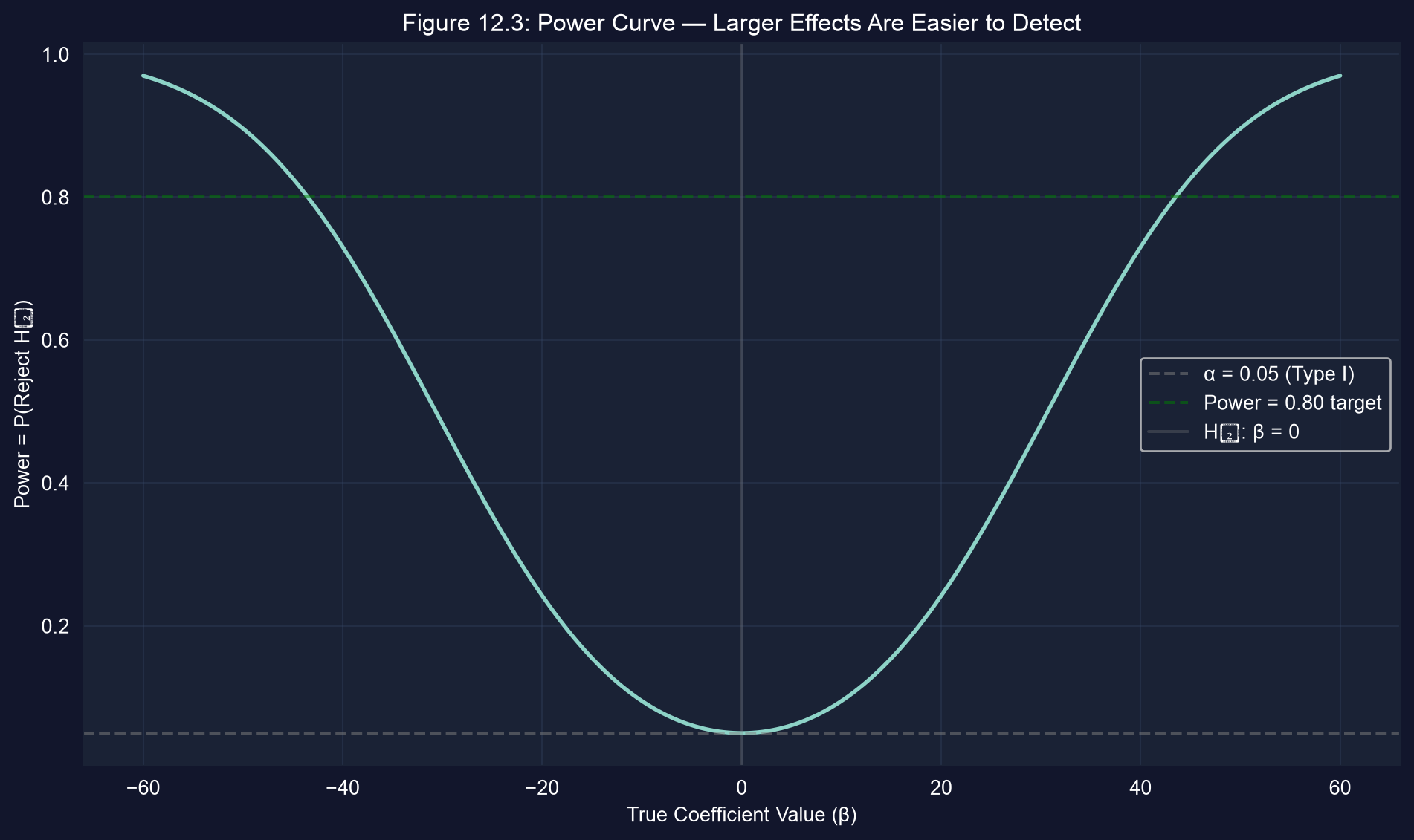
**Interpreting Figure 12.3:**
The power function shows how test power varies with the true coefficient value. Here's what each feature means:
**Key Features of the Curve:**
1. **At β = 0 (vertical gray line)**:
- Power = α = 0.05
- This is the Type I error rate
- When H₀ is true, we reject 5% of the time (false positives)
2. **As |β| increases (moving away from 0)**:
- Power increases rapidly
- Larger effects are easier to detect
- Curve approaches 1.0 (certain detection)
3. **Symmetry around zero**:
- Power is same for β = 30 and β = -30
- Two-sided test treats positive and negative effects equally
- One-sided tests would have asymmetric power
4. **The 0.80 threshold (green dashed line)**:
- Standard target: 80% power
- Means 20% chance of Type II error (β = 0.20)
- In this example: Need |β| ≈ 44 to achieve 80% power
**What This Means for Study Design:**
Given the parameters (n=30, SE=15, α=0.05):
- **Small effects** (|β| < 15):
- Power < 50%
- More likely to **miss** the effect than detect it
- Study is underpowered
- **Medium effects** (|β| ≈ 44):
- Power ≈ 80%
- Good chance of detection
- Standard benchmark for adequate power
- **Large effects** (|β| > 56):
- Power > 95%
- Almost certain detection
- Study is well-powered
**Sample Size Implications:**
To detect smaller effects, you need larger samples:
- **Double the sample** (n=60) → Can detect smaller effects with same power
- Minimum detectable effect shrinks in proportion to 1/√n
- To halve minimum detectable effect, need **4× the sample size**
**The Power-Sample Size Relationship:**
For a given effect size β:
- Power increases with √n
- To go from 50% to 80% power: Need ≈ 2× the sample
- To go from 80% to 95% power: Need ≈ 1.7× the sample again
**Practical Applications:**
1. **Pre-study planning**:
- Specify minimum effect of interest
- Calculate required sample size for 80% power
- Avoid underpowered studies
2. **Post-study interpretation**:
- Non-significant result with low power: Inconclusive (not evidence of no effect)
- Non-significant result with high power: Evidence against large effects
- Significant result: Good, but consider magnitude and practical significance
3. **Publication decisions**:
- Underpowered studies contribute to publication bias
- Meta-analyses should weight by precision and power
- Replication studies should be well-powered
**Common Mistakes to Avoid:**
1. Treating non-significant results as "proof of no effect"
- Non-significance in underpowered study is uninformative
2. Conducting multiple underpowered studies instead of one well-powered study
- Wastes resources and leads to false negatives
3. Post-hoc power analysis
- Don't calculate power after seeing results (circular reasoning)
- Do it before data collection
**The Bottom Line:**
This power curve illustrates a fundamental truth:
- **Smaller effects require larger samples to detect**
- With n=30 and SE=15, we can reliably detect effects of |β| ≥ 44 (where power reaches 80%)
- For smaller effects, we'd need more data or reduced noise (lower σ)
```{python}
# 12.5 BEST ESTIMATION METHODS — quick reference

print("When is OLS 'best'?\n")

print("1. Gauss-Markov Theorem")
print("   Under assumptions 1-4, OLS is BLUE: the minimum-variance")
print("   linear unbiased estimator.\n")

print("2. When assumptions fail")
print("   Heteroskedasticity -> Weighted Least Squares (WLS)")
print("   Autocorrelation     -> GLS with AR errors")
print("   Both                -> Feasible GLS (FGLS)\n")

print("3. Practical considerations")
print("   Efficiency gains are often modest, and misspecifying the error")
print("   structure can hurt, so most applied work uses OLS + robust SEs.\n")

print("4. Maximum Likelihood")
print("   Under normally distributed errors, MLE coincides with OLS")
print("   for the linear regression model.")
```
> **Key Concept 12.6: Feasible Generalized Least Squares**
>
> When error variance is not constant (heteroskedasticity) or errors are correlated (autocorrelation), OLS remains unbiased but is no longer the most efficient estimator. Feasible GLS (FGLS) models the error structure and can achieve lower variance. However, FGLS requires correctly specifying the error structure — in practice, OLS with robust SEs is preferred for its simplicity and robustness to misspecification.
## 12.6 Best Confidence Intervals
**What makes a confidence interval "best"?**
A 95% CI is "best" if it:
1. Has correct coverage: Contains true parameter 95% of the time
2. Has minimum width among all CIs with correct coverage
**Standard approach**: $\hat{\beta}_j \pm t_{n-k, \alpha/2} \times se(\hat{\beta}_j)$
- Width determined by $se(\hat{\beta}_j)$
- Shortest CI comes from most efficient estimator
**Alternative approaches**:
**1. Bootstrap confidence intervals**
- Resample data many times (e.g., 1000 replications)
- Re-estimate model for each resample
- Use distribution of bootstrap estimates
- Percentile method: 2.5th and 97.5th percentiles
- Advantages: No distributional assumptions, works for complex statistics
**2. Bayesian credible intervals**
- Based on posterior distribution
- Direct probability interpretation
- Incorporates prior information
**When assumptions fail**:
- Use robust SEs → wider but valid intervals
- Bootstrap → more accurate coverage in small samples
- Asymptotic approximations may be poor in small samples
> **Key Concept 12.7: Bootstrap Confidence Intervals**
>
> The bootstrap resamples the original data (with replacement) many times to estimate the sampling distribution of a statistic. Bootstrap CIs don't rely on normality or large-sample approximations, making them especially useful with small samples, skewed distributions, or non-standard estimators where analytical formulas aren't available.
## 12.7 Best Tests
**Type I and Type II errors**:
| Decision | $H_0$ True | $H_0$ False |
|----------|------------|-------------|
| Reject $H_0$ | Type I error (α) | Correct |
| Don't reject | Correct | Type II error (β) |
**Type I error** (false positive):
- Reject $H_0$ when it's true
- Probability = significance level α (e.g., 0.05)
- We control this directly
**Type II error** (false negative):
- Fail to reject $H_0$ when it's false
- Probability = β
- Harder to control
**Test power** = 1 - β
- Probability of correctly rejecting false $H_0$
- Higher power is better
**Trade-off**:
- Decreasing α (stricter test) → increases β (lower power)
- Solution: Fix α, maximize power
**Most powerful test**:
- Among all tests with size α, has highest power
- For linear regression: Use most efficient estimator
**The Trinity of Tests** (asymptotically equivalent):
1. **Wald test**: Based on unrestricted estimates
2. **Likelihood Ratio (LR) test**: Compares likelihoods
3. **Lagrange Multiplier (LM) test**: Based on restricted estimates
**Multiple testing**:
- Testing many hypotheses inflates Type I error
- Solutions: Bonferroni correction, FDR control
### Illustration: Power of a Test
Let's visualize how test power depends on the true effect size.
```{python}
# Figure 12.3: power curve — how the chance of detecting an effect grows with its size
alpha   = 0.05
se_test = 15                              # hypothetical standard error
n_test  = 30
t_crit  = stats.t.ppf(1 - alpha / 2, df=n_test - 1)

beta_range = np.linspace(-60, 60, 500)
power = []
for beta_true in beta_range:
    ncp = beta_true / se_test             # non-centrality parameter
    power_val = 1 - (stats.t.cdf(t_crit - ncp, df=n_test - 1)
                     - stats.t.cdf(-t_crit - ncp, df=n_test - 1))
    power.append(power_val)

fig, ax = plt.subplots(figsize=(10, 6))
ax.plot(beta_range, power, linewidth=2)
ax.axhline(0.05, color='gray', linestyle='--', alpha=0.5, label='α = 0.05 (Type I)')
ax.axhline(0.80, color='green', linestyle='--', alpha=0.5, label='Power = 0.80 target')
ax.axvline(0, color='gray', linestyle='-', alpha=0.3, label='H₀: β = 0')
ax.set_xlabel('True Coefficient Value (β)')
ax.set_ylabel('Power = P(Reject H₀)')
ax.set_title('Figure 12.3: Power Curve — Larger Effects Are Easier to Detect')
ax.legend()
ax.grid(True, alpha=0.3)
plt.tight_layout()
plt.show()
```
> **Key Concept 12.8: Type I and Type II Errors**
>
> Type I error (false positive) means rejecting a true $H_0$; its probability equals the significance level $\alpha$. Type II error (false negative) means failing to reject a false $H_0$. Power = $1 - P(\text{Type II})$ measures the ability to detect true effects. The most powerful test for a given size uses the most precise estimator — another reason efficient estimation matters beyond point estimates.
## Key Takeaways
**Robust Standard Errors:**
- When error variance is non-constant, default SEs are invalid — use heteroskedastic-robust (HC1) SEs for cross-sectional data
- With grouped observations, use cluster-robust SEs with $G-1$ degrees of freedom (not $N-k$)
- For time series with autocorrelated errors, use HAC (Newey-West) SEs with lag length $m \approx 0.75 \times T^{1/3}$
- Coefficient estimates are unchanged; only SEs, $t$-statistics, and CIs change
**Prediction:**
- Predicting the conditional mean $E[y|x^*]$ is more precise than predicting an individual outcome $y|x^*$
- Forecast variance = conditional mean variance + $\text{Var}(u^*)$, so prediction intervals are always wider
- Even with precise coefficients, individual forecasts are imprecise because we cannot predict $u^*$
- Policy decisions should be based on average outcomes (precise) rather than individual predictions (imprecise)
**Nonrepresentative Samples:**
- Sample selection on $Y$ can bias OLS estimates; selection on $X$ is less harmful
- Survey weights can adjust for known selection, but unknown selection remains problematic
**Best Estimation:**
- Under correct assumptions, OLS is BLUE (Gauss-Markov); when assumptions fail, FGLS is more efficient
- In practice, most studies use OLS with robust SEs — accepting a small efficiency loss for simplicity
**Best Confidence Intervals:**
- Bootstrap methods resample the data to estimate the sampling distribution without relying on normality
- Particularly useful with small samples or non-normal errors
**Best Tests:**
- Type I error = false positive (rejecting true $H_0$); Type II error = false negative
- Power = $1 - P(\text{Type II})$; the most powerful test uses the most precise estimator
- Higher power comes from larger samples, more variation in regressors, and lower noise
**Python tools used:** `pyfixest` (feols, HC1, predictions), `statsmodels` (HAC SEs, ACF plots), `scipy.stats` (distributions), `matplotlib`/`seaborn` (correlograms, prediction plots)
**Python Libraries and Code:**
This single code block reproduces the core workflow of Chapter 12. It is self-contained — copy it into an empty notebook and run it to review the complete pipeline from robust standard errors to prediction intervals, HAC inference, power analysis, and bootstrap confidence intervals.
```python
# =============================================================================
# CHAPTER 12 CHEAT SHEET: Further Topics in Multiple Regression
# =============================================================================

# --- Libraries ---
import pandas as pd                       # data loading and manipulation
import numpy as np                        # numerical operations
import matplotlib.pyplot as plt           # creating plots and visualizations
import pyfixest as pf                     # fast estimation with robust SEs
from scipy import stats                   # statistical distributions for CIs and power
from statsmodels.graphics.tsaplots import plot_acf  # autocorrelation plots

# =============================================================================
# STEP 1: Load house price data from a URL
# =============================================================================
# pd.read_stata() reads Stata .dta files directly from the web
url_house = "https://raw.githubusercontent.com/quarcs-lab/data-open/master/AED/AED_HOUSE.DTA"
data_house = pd.read_stata(url_house)

print(f"Dataset: {data_house.shape[0]} observations, {data_house.shape[1]} variables")
print(data_house[['price', 'size', 'bedrooms', 'bathrooms', 'lotsize', 'age']].describe().round(2))

# =============================================================================
# STEP 2: OLS regression with default standard errors
# =============================================================================
# Default SEs assume homoskedasticity (constant error variance)
model_default = pf.feols('price ~ size + bedrooms + bathrooms + lotsize + age + monthsold', data=data_house)

print(f"\nR-squared: {model_default._r2:.4f}")
print(f"Size effect (default): ${model_default.coef()['size']:,.2f} per sq ft")
model_default.summary()

# =============================================================================
# STEP 3: Robust (HC1) standard errors — compare with default
# =============================================================================
# HC1 SEs correct for heteroskedasticity without changing coefficient estimates
# Only the SEs, t-statistics, and confidence intervals change
model_robust = pf.feols('price ~ size + bedrooms + bathrooms + lotsize + age + monthsold', data=data_house, vcov='HC1')

# SE ratio: how much heteroskedasticity affects each coefficient's uncertainty
print(f"{'Variable':<14} {'Coef':>10} {'Default SE':>12} {'Robust SE':>12} {'Ratio':>8}")
print("-" * 58)
for var in model_default.coef().index:
    coef  = model_default.coef()[var]
    se_d  = model_default.se()[var]
    se_r  = model_robust.se()[var]
    ratio = se_r / se_d                   # ratio > 1 → default was too optimistic
    print(f"{var:<14} {coef:>10.2f} {se_d:>12.2f} {se_r:>12.2f} {ratio:>8.3f}")

# =============================================================================
# STEP 4: Prediction — conditional mean CI vs. individual forecast PI
# =============================================================================
# Predicting E[y|x*] is more precise than predicting an individual y|x*
model_simple = pf.feols('price ~ size', data=data_house)

# Predict for a 2000 sq ft house
new_house = pd.DataFrame({'size': [2000]})
pred_value = model_simple.predict(newdata=new_house)[0]

s_e = np.sqrt(np.sum(model_simple._u_hat**2) / (int(model_simple._N) - len(model_simple.coef())))    # RMSE — irreducible individual uncertainty

n_s = int(model_simple._N)
k_s = len(model_simple.coef())
t_crit_pred = stats.t.ppf(0.975, n_s - k_s)

print(f"\nPredicted price (2000 sq ft): ${pred_value:,.0f}")
print(f"95% PI for individual Y:  [${pred_value - t_crit_pred * s_e:,.0f}, "
      f"${pred_value + t_crit_pred * s_e:,.0f}]")
print(f"\nRMSE (s_e): ${s_e:,.0f} — PI can never be narrower than ±1.96 × s_e")

# Visualize: fitted line with approximate PI
sizes_sorted = data_house[['size']].sort_values('size')
pred_all = model_simple.predict(newdata=sizes_sorted)

fig, ax = plt.subplots(figsize=(10, 6))
ax.scatter(data_house['size'], data_house['price'], s=50, alpha=0.6, label='Actual')
ax.plot(sizes_sorted['size'], pred_all, color='red', linewidth=2, label='Fitted line')
ax.fill_between(sizes_sorted['size'],
                pred_all - t_crit_pred * s_e,
                pred_all + t_crit_pred * s_e,
                color='blue', alpha=0.1, label='95% PI (individual)')
ax.set_xlabel('House Size (sq ft)')
ax.set_ylabel('House Price ($)')
ax.set_title('Prediction Interval (pyfixest)')
ax.legend()
ax.grid(True, alpha=0.3)
plt.tight_layout()
plt.show()

# =============================================================================
# STEP 5: HAC (Newey-West) standard errors for time series
# =============================================================================
# Time series errors are often autocorrelated — HAC SEs account for this
url_gdp = "https://raw.githubusercontent.com/quarcs-lab/data-open/master/AED/AED_REALGDPPC.DTA"
data_gdp = pd.read_stata(url_gdp)

growth = data_gdp['growth'].dropna()      # drop initial missing growth values
mean_growth = growth.mean()
n_gdp       = len(growth)
lag_length   = int(0.75 * n_gdp**(1/3))  # rule of thumb: m = 0.75 × T^(1/3)

# Compare default SE vs. HAC SE for the mean
se_default = growth.std() / np.sqrt(n_gdp)
y = growth
X = np.ones(n_gdp)
# Note: For HAC SEs on the mean (intercept-only model), we use statsmodels
from statsmodels.regression.linear_model import OLS as smOLS
model_hac = smOLS(y, X).fit(cov_type='HAC', cov_kwds={'maxlags': lag_length})

print(f"\nGDP Growth: mean = {mean_growth:.4f}")
print(f"Default SE (no autocorrelation): {se_default:.6f}")
print(f"HAC SE (lag = {lag_length}):            {model_hac.bse.iloc[0]:.6f}")
print(f"Ratio HAC/Default: {model_hac.bse.iloc[0] / se_default:.3f}")

# Correlogram — visualize autocorrelation structure
fig, ax = plt.subplots(figsize=(10, 6))
plot_acf(growth, lags=10, ax=ax, alpha=0.05)
ax.set_xlabel('Lag')
ax.set_ylabel('Autocorrelation')
ax.set_title('Correlogram of GDP Growth')
plt.tight_layout()
plt.show()

# =============================================================================
# STEP 6: Power curve — Type I vs. Type II error tradeoff
# =============================================================================
# Power = P(reject H₀ | H₀ is false) — depends on true effect size
alpha = 0.05
se_test = 15                              # hypothetical standard error
n_test  = 30
t_crit  = stats.t.ppf(1 - alpha / 2, df=n_test - 1)

# Power as a function of the true coefficient
beta_range = np.linspace(-60, 60, 500)
power = []
for beta_true in beta_range:
    ncp = beta_true / se_test             # non-centrality parameter
    # Two-sided test: reject if |t| > t_crit
    power_val = 1 - (stats.t.cdf(t_crit - ncp, df=n_test - 1)
                      - stats.t.cdf(-t_crit - ncp, df=n_test - 1))
    power.append(power_val)

fig, ax = plt.subplots(figsize=(10, 6))
ax.plot(beta_range, power, linewidth=2)
ax.axhline(0.05, color='gray', linestyle='--', alpha=0.5, label='α = 0.05 (Type I)')
ax.axhline(0.80, color='green', linestyle='--', alpha=0.5, label='Power = 0.80 target')
ax.axvline(0, color='gray', linestyle='-', alpha=0.3, label='H₀: β = 0')
ax.set_xlabel('True Coefficient Value (β)')
ax.set_ylabel('Power = P(Reject H₀)')
ax.set_title('Power Curve: Larger Effects Are Easier to Detect')
ax.legend()
ax.grid(True, alpha=0.3)
plt.tight_layout()
plt.show()

# =============================================================================
# STEP 7: Bootstrap confidence intervals — no distributional assumptions
# =============================================================================
# Resample data with replacement to estimate the sampling distribution of β
np.random.seed(42)
n_boot = 1000
boot_slopes = []

for _ in range(n_boot):
    boot_sample = data_house.sample(n=len(data_house), replace=True)
    boot_model  = pf.feols('price ~ size', data=boot_sample)
    boot_slopes.append(boot_model.coef()['size'])

# Percentile method: 95% CI = [2.5th, 97.5th percentile]
ci_lower = np.percentile(boot_slopes, 2.5)
ci_upper = np.percentile(boot_slopes, 97.5)
ols_slope = model_simple.coef()['size']

print(f"\nOLS slope (size): {ols_slope:.4f}")
print(f"Bootstrap 95% CI: [{ci_lower:.4f}, {ci_upper:.4f}]")
print(f"Analytical 95% CI: [{model_simple.confint().loc['size'].iloc[0]:.4f}, "
      f"{model_simple.confint().loc['size'].iloc[1]:.4f}]")

fig, ax = plt.subplots(figsize=(10, 6))
ax.hist(boot_slopes, bins=40, edgecolor='black', alpha=0.7)
ax.axvline(ols_slope, color='red', linewidth=2, label=f'OLS estimate: {ols_slope:.4f}')
ax.axvline(ci_lower, color='green', linewidth=2, linestyle='--', label=f'2.5th pctl: {ci_lower:.4f}')
ax.axvline(ci_upper, color='green', linewidth=2, linestyle='--', label=f'97.5th pctl: {ci_upper:.4f}')
ax.set_xlabel('Bootstrap Slope Estimates')
ax.set_ylabel('Frequency')
ax.set_title('Bootstrap Distribution of Size Coefficient (1000 replications)')
ax.legend()
ax.grid(True, alpha=0.3)
plt.tight_layout()
plt.show()
```
**Try it yourself!** Copy this code into an empty Google Colab notebook and run it: [Open Colab](https://colab.research.google.com/notebooks/empty.ipynb)
**Next Steps:**
- **Chapter 13**: Case studies that apply the full multiple regression toolkit to real economic questions
- **Chapter 14**: Regression with indicator (dummy) variables — handling qualitative explanatory variables
- **Chapter 15**: Regression with transformed variables (logs, quadratics, and interactions)
- **Chapter 16**: Checking the model and data — diagnostics for specification and influential observations
Congratulations on completing Chapter 12! You now understand advanced inference methods for handling real-world data challenges.
> **Common Mistakes to Avoid**
>
> - **Ignoring heteroskedasticity**: Invalidates standard errors and hypothesis tests
> - **Using clustered standard errors incorrectly**: Requires sufficient clusters (rule of thumb: 30+)
> - **Confusing GLS and OLS**: GLS is more efficient under heteroskedasticity but requires correct specification
## Practice Exercises
Test your understanding of advanced inference topics.
---
**Exercise 1: Choosing Standard Errors**
For each scenario, identify the appropriate type of standard errors:
a) Cross-sectional survey of 500 households with varying income levels.
b) Panel data on 50 schools over 10 years, where student outcomes within a school are correlated.
c) Monthly GDP growth data for 20 years, where this quarter's shock affects next quarter.
d) A randomized experiment with 200 independent observations and constant error variance.
---
**Exercise 2: Point Prediction**
A fitted regression model gives $\widehat{y} = 10 + 2x_2 + 3x_3$ with $n = 200$ and $s_e = 2.0$.
a) Predict $y$ when $x_2 = 5$ and $x_3 = 3$.
b) Is this a prediction of the conditional mean or an individual outcome?
---
**Exercise 3: Conditional Mean CI**
Using the model from Exercise 2, suppose $se(\widehat{y}_{cm}) = 0.8$ at $x_2 = 5, x_3 = 3$.
a) Construct an approximate 95% confidence interval for $E[y|x_2=5, x_3=3]$.
b) How would this interval change if the sample size doubled (assume SE shrinks by $\sqrt{2}$)?
---
**Exercise 4: Individual Forecast CI**
Continuing from Exercise 3, construct a 95% prediction interval for an individual $y$ at $x_2 = 5, x_3 = 3$.
a) Compute $se(\widehat{y}_f) = \sqrt{se(\widehat{y}_{cm})^2 + s_e^2}$.
b) Construct the prediction interval.
c) Why is this interval so much wider than the confidence interval for the conditional mean?
---
**Exercise 5: Robust vs. Default Inference**
A regression yields the following results:
| Variable | Coefficient | Default SE | Robust SE |
|----------|------------|-----------|----------|
| $x_2$ | 5.0 | 2.0 | 3.5 |
| $x_3$ | 7.0 | 2.0 | 1.8 |
a) Compute the $t$-statistic for each variable using default and robust SEs.
b) At $\alpha = 0.05$, which variables are significant under each type of SE?
c) What does the change in SEs suggest about heteroskedasticity?
---
**Exercise 6: Type I/II Error Tradeoff**
A researcher tests $H_0: \beta = 0$ at three significance levels: $\alpha = 0.01, 0.05, 0.10$.
a) As $\alpha$ decreases, what happens to the probability of Type I error?
b) As $\alpha$ decreases, what happens to the probability of Type II error?
c) If it's very costly to miss a true effect (high cost of Type II error), should you use a smaller or larger $\alpha$? Explain.
## Case Studies
### Case Study 1: Robust Inference for Cross-Country Productivity
In this case study, you will apply robust inference methods to cross-country productivity data. You'll compare default and robust standard errors, make predictions for specific countries, and assess how methodological choices affect conclusions about productivity determinants.
**Dataset:** Mendez Convergence Clubs Data
- **Source:** Mendez (2020), 108 countries, 1990-2014
- **Key variables:**
- `lp` — Labor productivity (GDP per worker)
- `kl` — Physical capital per worker
- `h` — Human capital index
- `region` — Geographic region (for clustering)
**Research question:** Do conclusions about productivity determinants change when using robust standard errors? How precisely can we predict productivity for a specific country?
```python
# Load the Mendez convergence clubs dataset
url = "https://raw.githubusercontent.com/quarcs-lab/mendez2020-convergence-clubs-code-data/master/assets/dat.csv"
dat = pd.read_csv(url)
dat_2014 = dat[dat['year'] == 2014].dropna(subset=['lp', 'kl', 'h']).copy()
dat_2014['ln_lp'] = np.log(dat_2014['lp'])
dat_2014['ln_kl'] = np.log(dat_2014['kl'])
print(f"Cross-section sample: {len(dat_2014)} countries (year 2014)")
```
#### Task 1: Default vs. Robust Standard Errors (Guided)
Compare default and heteroskedastic-robust standard errors.
```python
# Estimate model with default SEs
model = pf.feols('ln_lp ~ ln_kl + h', data=dat_2014)
print("Default SEs:")
model.summary()

# Estimate with HC1 robust SEs (pyfixest handles this at estimation time)
model_robust = pf.feols('ln_lp ~ ln_kl + h', data=dat_2014, vcov='HC1')
print("\nRobust SEs:")
model_robust.summary()
```
**Questions:**
- How do the standard errors change? Which variables are affected most?
- Do any significance conclusions change between default and robust SEs?
#### Task 2: Cluster-Robust SEs by Region (Guided)
Estimate with cluster-robust standard errors grouped by geographic region.
```python
# Cluster-robust SEs by region
model_cluster = pf.feols('ln_lp ~ ln_kl + h', data=dat_2014, vcov={'CRV1': 'region'})
print("Cluster-Robust SEs (by region):")
model_cluster.summary()

# Compare all three SE types
print("\nSE Comparison:")
for var in ['Intercept', 'ln_kl', 'h']:
    print(f"  {var}: Default={model.se()[var]:.4f}, HC1={model_robust.se()[var]:.4f}, Cluster={model_cluster.se()[var]:.4f}")
```
**Questions:**
- Are cluster-robust SEs larger or smaller than HC1 SEs? Why?
- How many clusters (regions) are there? Is this enough for reliable cluster-robust inference?
> **Key Concept 12.9: Choosing the Right Standard Errors**
>
> The choice of standard errors depends on the data structure: HC1 for cross-sectional data with potential heteroskedasticity, cluster-robust when observations are grouped (e.g., countries within regions), and HAC for time series. With cross-country data, cluster-robust SEs by region account for the possibility that countries in the same region share unobserved shocks.
#### Task 3: Predict Conditional Mean (Semi-guided)
Predict average productivity for a country with median capital and human capital values.
```python
# Get median values
median_ln_kl = dat_2014['ln_kl'].median()
median_h = dat_2014['h'].median()
print(f"Median ln(kl) = {median_ln_kl:.3f}, Median h = {median_h:.3f}")

# Predict conditional mean with CI
pred_data = pd.DataFrame({'ln_kl': [median_ln_kl], 'h': [median_h]})
pred_value = model.predict(newdata=pred_data)
print(f"Predicted ln(lp): {pred_value[0]:.3f}")
```
**Questions:**
- What is the predicted $\ln(\text{lp})$ for a median country? Convert back to levels.
- How narrow is the 95% CI for the conditional mean?
#### Task 4: Forecast Individual Country (Semi-guided)
Construct a prediction interval for an individual country's productivity.
```python
# Approximate 95% prediction interval for an individual country
# (dominant-term approximation: pred +/- t * s_e, following section 12.3)
s_e    = np.sqrt(np.sum(model._u_hat**2) / (int(model._N) - len(model.coef())))
t_crit = stats.t.ppf(0.975, int(model._N) - len(model.coef()))
pi_lower = pred_value[0] - t_crit * s_e
pi_upper = pred_value[0] + t_crit * s_e
print(f"Point prediction (conditional mean): {pred_value[0]:.3f}")
print(f"Approx. 95% PI for an individual country: [{pi_lower:.3f}, {pi_upper:.3f}]")
print(f"RMSE (s_e): {s_e:.3f} -- the PI can never be narrower than +/- t*s_e")
```
**Questions:**
- How much wider is the prediction interval compared to the confidence interval?
- Why can't we predict an individual country's productivity precisely even with good data?
#### Task 5: Model Comparison with Robust Inference (Independent)
Compare nested models using robust inference.
**Your tasks:**
1. Estimate three models: (a) $\ln(\text{lp}) \sim \ln(\text{kl})$ only, (b) $\ln(\text{lp}) \sim \text{h}$ only, (c) both regressors
2. For each model, report both default and HC1 robust standard errors
3. Do the significance conclusions change between default and robust SEs for any model?
4. Compare prediction interval widths across models — does adding variables improve individual predictions?
*Hint: Use `pf.feols(..., vcov='HC1')` for robust SEs and `model.predict(newdata=...)` for predictions.*
#### Task 6: Policy Brief on Inference Robustness (Independent)
Write a 200-300 word policy brief summarizing your findings.
**Your brief should address:**
1. How do conclusions about productivity determinants change with robust standard errors?
2. What is the practical difference between cluster-robust and HC1 SEs in this context?
3. How precisely can we predict productivity for a specific country vs. a group of countries?
4. What recommendations would you make about standard error choices for cross-country studies?
5. What are the limitations of these inference methods (what don't they fix)?
> **Key Concept 12.10: Robust Methods Don't Fix Everything**
>
> Robust standard errors correct for heteroskedasticity and clustering, but they don't address omitted variable bias, reverse causality, or measurement error. A coefficient estimate with a perfectly robust SE is still biased if the model is misspecified. Robust inference ensures valid $p$-values and CIs *conditional on the model being correct* — it's a necessary but not sufficient condition for credible empirical work.
#### What You've Learned
In this case study, you applied advanced inference methods to cross-country productivity data:
- Compared default, heteroskedastic-robust, and cluster-robust standard errors
- Observed how SE choices affect significance conclusions
- Predicted conditional means with narrow CIs and individual outcomes with wide PIs
- Connected robust inference methods to practical policy questions
These tools ensure your empirical conclusions are reliable under realistic data conditions.
### Case Study 2: Robust Prediction of Municipal Development
In Chapters 10-11, we estimated multiple regression models predicting municipal development from nighttime lights and satellite embeddings, and tested the statistical significance of these predictors. Now we apply Chapter 12's tools for **robust inference** and **prediction**---crucial for translating satellite models into practical SDG monitoring tools.
**The Data**: The [DS4Bolivia project](https://github.com/quarcs-lab/ds4bolivia) provides a comprehensive dataset covering 339 Bolivian municipalities with over 350 variables, including the Municipal Sustainable Development Index (IMDS), nighttime lights per capita, and 64 satellite embedding dimensions. Here we focus on robust standard errors and prediction intervals for the satellite-development model.
#### Load the DS4Bolivia Data
Let's load the DS4Bolivia dataset and select the key variables for robust inference and prediction analysis.
```{python}
# Load the DS4Bolivia dataset
url_bol = "https://raw.githubusercontent.com/quarcs-lab/ds4bolivia/master/ds4bolivia_v20250523.csv"
bol = pd.read_csv(url_bol)

# Load and merge satellite image embeddings
url_sat = "https://raw.githubusercontent.com/quarcs-lab/ds4bolivia/master/satelliteEmbeddings/satelliteEmbeddings2017.csv"
sat = pd.read_csv(url_sat)
bol = bol.merge(sat[['asdf_id', 'A00', 'A10', 'A20', 'A30', 'A40']], on='asdf_id', how='left')

# Display basic information
print(f"Dataset shape: {bol.shape[0]} municipalities, {bol.shape[1]} variables")
print(f"Departments: {bol['dep'].nunique()} unique departments")

# Select key variables for this case study
key_vars = ['mun', 'dep', 'imds', 'ln_NTLpc2017',
            'A00', 'A10', 'A20', 'A30', 'A40']
bol_key = bol[key_vars].copy()

print(f"\nKey variables selected: {len(key_vars)}")
# FIRST 10 MUNICIPALITIES
print(bol_key.head(10).to_string())

# Variable descriptions
# KEY VARIABLE DESCRIPTIONS
descriptions = {
    'mun': 'Municipality name',
    'dep': 'Department (administrative region, 9 total)',
    'imds': 'Municipal Sustainable Development Index (0-100, composite of all SDGs)',
    'ln_NTLpc2017': 'Log of nighttime lights per capita (2017, satellite-based)',
    'A00-A40': 'Satellite image embedding dimensions (5 of 64 principal features)',
}
for var, desc in descriptions.items():
    print(f"  {var:20s} --- {desc}")
```
#### Task 1: Default vs Robust Standard Errors (Guided)
**Objective**: Estimate the satellite-development model with both default and HC1 robust standard errors and compare the results.
**Instructions**:
1. Estimate `imds ~ ln_NTLpc2017 + A00 + A10 + A20 + A30 + A40` with default standard errors
2. Re-estimate with HC1 robust standard errors (`vcov='HC1'`)
3. Compare standard errors side-by-side for each coefficient
4. Identify which coefficients have substantially different SEs under the two methods
**Apply what you learned in section 12.2**: Use `pf.feols()` for default SEs and `pf.feols(..., vcov='HC1')` for robust SEs.
```{python}
# Task 1: Default vs Robust Standard Errors
# ----------------------------------------------------------

# Prepare regression data (drop missing values)
reg_vars = ['imds', 'ln_NTLpc2017', 'A00', 'A10', 'A20', 'A30', 'A40']
reg_data = bol_key[reg_vars + ['dep']].dropna()
print(f"Regression sample: {len(reg_data)} municipalities (after dropping missing values)")

# Estimate with default standard errors
model_default = pf.feols('imds ~ ln_NTLpc2017 + A00 + A10 + A20 + A30 + A40', data=reg_data)

# Estimate with HC1 robust standard errors
model_hc1 = pf.feols('imds ~ ln_NTLpc2017 + A00 + A10 + A20 + A30 + A40', data=reg_data, vcov='HC1')

# COMPARISON: DEFAULT vs HC1 ROBUST STANDARD ERRORS
print(f"{'Variable':<18} {'Coef':>10} {'Default SE':>12} {'HC1 SE':>12} {'Ratio':>8}")
for var in model_default.coef().index:
    coef = model_default.coef()[var]
    se_def = model_default.se()[var]
    se_hc1 = model_hc1.se()[var]
    ratio = se_hc1 / se_def
    print(f"{var:<18} {coef:>10.4f} {se_def:>12.4f} {se_hc1:>12.4f} {ratio:>8.3f}")

print(f"\nR-squared: {model_default._r2:.4f}")
print(f"Adj. R-squared: {model_default._adj_r2:.4f}")
print(f"\nNote: Coefficients are identical --- only SEs change.")
print("Ratios > 1 mean the default SEs understated uncertainty (overstated precision) for that coefficient.")
```
#### Task 2: Cluster-Robust Standard Errors by Department (Guided)
**Objective**: Re-estimate the model with cluster-robust standard errors grouped by department.
**Instructions**:
1. Re-estimate using `vcov={'CRV1': 'dep'}` to cluster by department
2. Compare cluster-robust SEs with default and HC1 SEs
3. Discuss: Why might municipalities within a department share unobserved characteristics?
**Apply what you learned in section 12.2**: Cluster-robust SEs account for within-group correlation of errors. *Caution: with only 9 departments, this analysis sits well below the 30+ clusters rule of thumb (see the Common Mistakes box), so cluster-robust p-values here should be interpreted carefully.*
```{python}
# Task 2: Cluster-Robust Standard Errors by Department
# ----------------------------------------------------------

# Estimate with cluster-robust SEs by department
model_cluster = pf.feols('imds ~ ln_NTLpc2017 + A00 + A10 + A20 + A30 + A40', data=reg_data, vcov={'CRV1': 'dep'})

# COMPARISON: DEFAULT vs HC1 vs CLUSTER-ROBUST STANDARD ERRORS
print(f"{'Variable':<18} {'Coef':>10} {'Default SE':>12} {'HC1 SE':>12} {'Cluster SE':>12}")
for var in model_default.coef().index:
    coef = model_default.coef()[var]
    se_def = model_default.se()[var]
    se_hc1 = model_hc1.se()[var]
    se_clust = model_cluster.se()[var]
    print(f"{var:<18} {coef:>10.4f} {se_def:>12.4f} {se_hc1:>12.4f} {se_clust:>12.4f}")

n_clusters = reg_data['dep'].nunique()
print(f"\nNumber of clusters (departments): {n_clusters}")
print(f"Municipalities per department (avg): {len(reg_data) / n_clusters:.0f}")
```
> **Key Concept 12.11: Clustered Observations in Spatial Data**
>
> Municipalities within the same department share geographic, institutional, and cultural characteristics that create **within-cluster correlation**. Standard OLS assumes independent errors, but when municipalities in La Paz share unobserved factors that affect development, their errors are correlated. Cluster-robust standard errors account for this correlation, typically producing *larger* SEs than default or HC1, reflecting the reduced effective sample size.
#### Task 3: Predict Conditional Mean (Semi-guided)
**Objective**: Use `model.predict()` to predict average IMDS for a municipality with median values of all predictors.
**Instructions**:
1. Calculate the median value of each predictor variable
2. Use `model_default.predict(newdata=...)` to predict IMDS at the median predictor values
3. Report the predicted value and its 95% confidence interval
4. Interpret: "For a typical municipality, we predict IMDS between X and Y"
**Apply what you learned in section 12.3**: The confidence interval for the conditional mean reflects estimation uncertainty only.
```{python}
# Task 3: Predict Conditional Mean
# ----------------------------------------------------------

# Your code here: Predict IMDS for a municipality with median predictor values
#
# Steps:
# 1. Calculate median values for each predictor
# 2. Create a DataFrame with those values
# 3. Use model_default.predict(newdata=...) to get prediction
# 4. Report and interpret

# Example structure:
# pred_vars = ['ln_NTLpc2017', 'A00', 'A10', 'A20', 'A30', 'A40']
# median_vals = reg_data[pred_vars].median()
# pred_data = pd.DataFrame([median_vals])
#
# pred_value = model_default.predict(newdata=pred_data)[0]
# print(f"Predicted IMDS (conditional mean): {pred_value:.2f}")
#
# # Note: pyfixest returns a point prediction. A full CI for the conditional
# # mean needs the fitted-value variance x0' V x0, which is beyond this
# # chapter, so here we report and interpret the point estimate.
# print(f"For a typical municipality with median predictors, we predict")
# print(f"an average IMDS of about {pred_value:.1f}.")
```
#### Task 4: Prediction Interval for an Individual Municipality (Semi-guided)
**Objective**: Compute the 95% prediction interval for an *individual* municipality (not just the mean) and compare it with the confidence interval.
**Instructions**:
1. Use `model_default.predict(newdata=...)` at the same median predictor values
2. Build an approximate 95% prediction interval as `pred ± t·s_e` using the model's residual standard error (RMSE), following section 12.3
3. Compare the width of the prediction interval with the confidence interval from Task 3
4. Explain why the prediction interval is wider
**Apply what you learned in section 12.3**: Individual predictions must account for the irreducible error $u^*$, making them fundamentally less precise than conditional mean predictions.
```{python}
# Task 4: Prediction Interval for an Individual Municipality
# ----------------------------------------------------------

# Your code here: Compute prediction interval and compare with CI
#
# Steps:
# 1. Use the same prediction from Task 3
# 2. Extract obs_ci_lower and obs_ci_upper for the prediction interval
# 3. Compare widths
# 4. Discuss why PI is wider

# Example structure:
# pred_vars = ['ln_NTLpc2017', 'A00', 'A10', 'A20', 'A30', 'A40']
# median_vals = reg_data[pred_vars].median()
# pred_data = pd.DataFrame([median_vals])
#
# pred_value = model_default.predict(newdata=pred_data)[0]
# s_e = np.sqrt(np.sum(model_default._u_hat**2) / (int(model_default._N) - len(model_default.coef())))
# t_crit = stats.t.ppf(0.975, int(model_default._N) - len(model_default.coef()))
# pi_lower = pred_value - t_crit * s_e
# pi_upper = pred_value + t_crit * s_e
#
# print("PREDICTION INTERVAL FOR AN INDIVIDUAL MUNICIPALITY")
# print(f"Predicted IMDS: {pred_value:.2f}")
# print(f"95% PI (individual): [{pi_lower:.2f}, {pi_upper:.2f}]  width = {pi_upper - pi_lower:.2f}")
# print(f"RMSE (s_e): {s_e:.2f} -- the PI can never be narrower than +/- t*s_e")
# print("\nThe prediction interval is wide because it includes the")
# print("irreducible uncertainty from the individual error term u*.")
```
> **Key Concept 12.12: Prediction Uncertainty for SDG Monitoring**
>
> Satellite-based prediction models can estimate *average* development patterns with reasonable precision (narrow confidence intervals for the conditional mean). However, predicting development for a *specific municipality* involves much greater uncertainty (wide prediction intervals) because individual municipalities deviate from the average relationship. For SDG monitoring, this means satellite predictions are more reliable for identifying broad patterns than for pinpointing the exact development level of any single municipality.
#### Task 5: Model Robustness Comparison (Independent)
**Objective**: Create a comprehensive comparison table showing coefficient estimates and standard errors under three specifications: default, HC1, and cluster-robust.
**Instructions**:
1. Create a formatted comparison table with coefficients, SEs, and significance stars under all three SE specifications
2. Identify whether any coefficients change sign or statistical significance across specifications
3. Discuss what the comparison reveals about model reliability
4. What does stability (or instability) across SE methods tell us about the trustworthiness of our satellite-development model?
**This extends Chapter 12 concepts**: You're systematically assessing how robust your conclusions are to different assumptions about the error structure.
```{python}
# Task 5: Model Robustness Comparison
# ----------------------------------------------------------

# Your code here: Create comprehensive comparison table
#
# Steps:
# 1. Extract coefficients and SEs from all three models
# 2. Compute t-statistics and significance levels for each
# 3. Create a formatted comparison table
# 4. Identify any changes in sign or significance

# Example structure:
# def sig_stars(pval):
#     if pval < 0.01: return '***'
#     elif pval < 0.05: return '**'
#     elif pval < 0.10: return '*'
#     else: return ''
#
#
# print("MODEL ROBUSTNESS: COEFFICIENT ESTIMATES AND STANDARD ERRORS")
#
# print(f"{'Variable':<16} {'Coef':>8} {'SE(Def)':>10} {'SE(HC1)':>10} {'SE(Clust)':>10} "
#       f"{'Sig(D)':>7} {'Sig(H)':>7} {'Sig(C)':>7}")
#
# for var in model_default.coef().index:
#     coef = model_default.coef()[var]
#     se_d = model_default.se()[var]
#     se_h = model_hc1.se()[var]
#     se_c = model_cluster.se()[var]
#     sig_d = sig_stars(model_default.pvalue()[var])
#     sig_h = sig_stars(model_hc1.pvalue()[var])
#     sig_c = sig_stars(model_cluster.pvalue()[var])
#     print(f"{var:<16} {coef:>8.4f} {se_d:>10.4f} {se_h:>10.4f} {se_c:>10.4f} "
#           f"{sig_d:>7} {sig_h:>7} {sig_c:>7}")
#
# print("Significance: *** p<0.01, ** p<0.05, * p<0.10")
#
# print("\nDo any coefficients change sign or significance?")
# print("What does this tell us about model reliability?")
```
#### Task 6: Prediction Brief (Independent)
**Objective**: Write a 200-300 word assessment of prediction uncertainty in satellite-based development models.
**Your brief should address:**
1. How much uncertainty exists in satellite-based development predictions?
2. Are prediction intervals narrow enough to be useful for policy targeting?
3. How does the confidence interval for the conditional mean compare with the prediction interval for individual municipalities?
4. What additional data or methods might reduce prediction uncertainty?
5. Should policymakers rely on satellite predictions for allocating development resources to specific municipalities?
**Connection to Research**: The DS4Bolivia project shows that satellite-based models achieve meaningful but imperfect predictive accuracy. Your analysis quantifies *how much uncertainty* remains and whether it is small enough for practical SDG monitoring applications.
```{python}
# Your code here: Additional analysis for the prediction brief
#
# You might want to:
# 1. Compare prediction intervals at different predictor values
#    (e.g., low-NTL vs high-NTL municipalities)
# 2. Calculate how many municipalities fall outside prediction intervals
# 3. Visualize actual vs predicted IMDS with confidence bands
#
# Example structure:
# # Actual vs predicted comparison
# reg_data['predicted'] = model_default.predict(reg_data)
# reg_data['residual'] = reg_data['imds'] - reg_data['predicted']
#
#
# print("PREDICTION ACCURACY SUMMARY")
#
# print(f"RMSE: {np.sqrt(np.sum(model_default._u_hat**2) / (int(model_default._N) - len(model_default.coef()))):.2f}")
# print(f"Mean IMDS: {reg_data['imds'].mean():.2f}")
# print(f"RMSE as % of mean: {100 * np.sqrt(np.sum(model_default._u_hat**2) / (int(model_default._N) - len(model_default.coef()))) / reg_data['imds'].mean():.1f}%")
# print(f"\nLargest over-prediction: {reg_data['residual'].min():.2f}")
# print(f"Largest under-prediction: {reg_data['residual'].max():.2f}")
```
#### What You've Learned from This Case Study
Through this analysis of robust inference and prediction for Bolivia's satellite-development model, you've practiced:
- **Robust SE comparison**: Compared default, HC1, and cluster-robust standard errors for the same model
- **Cluster-robust inference**: Accounted for within-department correlation among municipalities
- **Conditional mean prediction**: Predicted average IMDS with a narrow 95% confidence interval
- **Prediction intervals**: Quantified the much larger uncertainty in predicting individual municipalities
- **Model robustness assessment**: Evaluated whether conclusions change across different SE specifications
These tools are essential for translating satellite-based models into credible SDG monitoring instruments. Robust inference ensures your significance conclusions hold under realistic data conditions, while prediction intervals honestly communicate the limits of individual-level forecasting.
**Connection to future chapters**: In Chapter 14, we add *indicator variables* for departments to explicitly model regional differences in the satellite-development relationship.
---
**Well done!** You've now applied Chapter 12's advanced inference and prediction tools to the satellite-development model, quantifying both the reliability of your estimates and the precision of your predictions.