---
title: 8. Case Studies for Bivariate Regression
execute:
enabled: true
warning: false
---
**metricsAI: An Introduction to Econometrics with Python and AI in the Cloud**
*[Carlos Mendez](https://carlos-mendez.org)*
<img src="https://raw.githubusercontent.com/quarcs-lab/metricsai/main/images/ch08_visual_summary.jpg" alt="Chapter 08 Visual Summary" width="100%">
This notebook provides an interactive introduction to bivariate regression through real-world case studies. All code runs directly in Google Colab without any local setup.
[](https://colab.research.google.com/github/quarcs-lab/metricsai/blob/main/notebooks_colab/ch08_Case_Studies_for_Bivariate_Regression.ipynb)
<div class="chapter-resources">
<a href="https://www.youtube.com/watch?v=2hVGYcT9YE8" target="_blank" class="resource-btn">🎬 AI Video</a>
<a href="https://carlos-mendez.my.canva.site/s08-case-studies-for-bivariate-regression-pdf" target="_blank" class="resource-btn">✨ AI Slides</a>
<a href="https://cameron.econ.ucdavis.edu/aed/traedv1_08" target="_blank" class="resource-btn">📊 Cameron Slides</a>
<a href="https://app.edcafe.ai/quizzes/697867452f5d08069e049d1f" target="_blank" class="resource-btn">✏️ Quiz</a>
<a href="https://app.edcafe.ai/chatbots/6978a02d2f5d08069e0711d6" target="_blank" class="resource-btn">🤖 AI Tutor</a>
</div>
## Chapter Overview
This chapter demonstrates bivariate regression analysis through four compelling real-world applications. You'll gain both theoretical understanding and practical skills through hands-on Python examples.
**Design Note:** This chapter uses an integrated case study structure where sections 8.1-8.4 ARE the case studies (health economics, finance, macroeconomics). Unlike other chapters that have regular content sections plus a separate "Case Studies" section, CH08's entire focus is on applying regression to diverse real-world problems. This intentional structure maximizes hands-on experience with economic applications.
**What you'll learn:**
- Apply bivariate regression to cross-sectional data (health outcomes, expenditures)
- Estimate financial models (Capital Asset Pricing Model)
- Analyze macroeconomic relationships (Okun's Law)
- Use heteroskedasticity-robust standard errors
- Interpret economic and statistical significance
- Identify outliers and assess their influence
**Datasets used:**
- **AED_HEALTH2009.DTA**: Health outcomes and expenditures for 34 OECD countries (2009)
- **AED_CAPM.DTA**: Monthly stock returns for Coca-Cola, Target, Walmart (1983-2012)
- **AED_GDPUNEMPLOY.DTA**: Annual U.S. GDP growth and unemployment (1961-2019)
**Key economic questions:**
- Do higher health expenditures improve health outcomes?
- How does GDP relate to health spending across countries?
- What is the systematic risk (beta) of individual stocks?
- Does Okun's Law hold for U.S. macroeconomic data?
**Chapter outline:**
- 8.1 Health Outcomes Across Countries
- 8.2 Health Expenditures Across Countries
- 8.3 Capital Asset Pricing Model (CAPM)
- 8.4 Output and Unemployment (Okun's Law)
- Key Takeaways
- Practice Exercises
## Key Concepts
Five core ideas anchor this chapter. Skim them before you start, and come back when a term feels fuzzy. Each entry pairs a concrete example using the chapter's data with a non-technical analogy. Click a panel to expand it.
**Capital Asset Pricing Model (CAPM):** A workhorse finance model that explains an asset's expected excess return as a multiple of the market's expected excess return: $R_A - R_F = \alpha_A + \beta_A (R_M - R_F) + u$. The slope $\beta_A$ measures how much the asset moves with the market — its share of *systematic* risk.
::::: {.columns}
:::: {.column width="50%"}
::: {.callout-tip collapse="true" appearance="simple" title="Example"}
For 354 monthly observations on Coca-Cola from `data_capm` (1983–2012), the CAPM regression of `rko_rf` on `rm_rf` produces $\hat\beta = 0.61$ with $R^2 \approx 0.20$ — the market explains 20% of the variation in Coca-Cola's monthly excess returns, and Coke moves only 61 cents on the market's dollar.
:::
::::
:::: {.column width="50%"}
::: {.callout-note collapse="true" appearance="simple" title="Analogy"}
A small boat in a busy harbor rises and falls with the tide. The CAPM is a way of asking *how much* of the boat's bobbing comes from the tide itself — not from what's happening on board (engine surges, passenger weight). $\beta$ is the boat's coupling to the tide; $R^2$ is the share of motion the tide can explain.
:::
::::
:::::
**Excess Return ($R - R_F$):** The return on an asset *above and beyond* the risk-free rate $R_F$ (e.g., a 1-month U.S. Treasury bill). Investors demand this premium for bearing risk; CAPM tries to explain it as compensation for *systematic* risk only.
::::: {.columns}
:::: {.column width="50%"}
::: {.callout-tip collapse="true" appearance="simple" title="Example"}
In `data_capm`, Coca-Cola's average monthly return minus the risk-free Treasury rate gives `rko_rf` — the asset's excess return — averaging slightly above zero. The regressor `rm_rf` does the same for the market. Subtracting the safe alternative is what makes the regression about *risk-adjusted* compensation, not raw price changes.
:::
::::
:::: {.column width="50%"}
::: {.callout-note collapse="true" appearance="simple" title="Analogy"}
A retail "deal" is the price discount you get *above* the everyday store price. A 20% sale on a chair worth \$100 is a \$20 excess saving. Excess returns are the same idea applied to investments — only the part that actually beats the safest baseline counts as a "deal" worth taking risk for.
:::
::::
:::::
**Alpha (Jensen's Alpha):** The intercept $\alpha$ in a CAPM regression — the average excess return the asset earned that the market factor *cannot* explain. Pure CAPM theory predicts $\alpha = 0$; a statistically significant non-zero alpha is interpreted as risk-adjusted out- or under-performance.
::::: {.columns}
:::: {.column width="50%"}
::: {.callout-tip collapse="true" appearance="simple" title="Example"}
The fitted Coca-Cola CAPM gives $\hat\alpha \approx 0.0068$ — about $0.68\%$ per month, or roughly $8.2\%$ annualised, in excess of what the market beta predicts. Tested against $H_0: \alpha = 0$, it is statistically significant — a textbook "alpha puzzle" for risk-adjusted out-performance over 1983–2012.
:::
::::
:::: {.column width="50%"}
::: {.callout-note collapse="true" appearance="simple" title="Analogy"}
A chef serves a tasting menu where every dish has a published expected flavor. Alpha is the surprise extra spice the chef adds that the menu didn't promise — credit not earned by following the recipe. Statistically significant alpha means the chef's secret seasoning is real, not just a one-night accident.
:::
::::
:::::
**Cross-Sectional Regression:** A regression run on a snapshot of many units observed at *one* moment — countries, firms, households, etc. Variation in $x$ across the units identifies the slope, and standard errors typically need a heteroskedasticity-robust adjustment because units differ in noise level.
::::: {.columns}
:::: {.column width="50%"}
::: {.callout-tip collapse="true" appearance="simple" title="Example"}
The first case study runs a cross-sectional regression of `lifeexp` on `hlthpc` across 34 OECD countries observed in 2009 — one year, 34 units. The fitted slope of $0.00111$ implies each extra \$1{,}000 in per-capita health spending is associated with about $1.1$ extra years of life expectancy, with $t \approx 3.9$.
:::
::::
:::: {.column width="50%"}
::: {.callout-note collapse="true" appearance="simple" title="Analogy"}
A photographer lines up 34 students for a class portrait — one frame, one click. Each face shows a different height, hair colour, expression. Cross-sectional regression studies *those* differences across the classmates: how does one trait covary with another in this single frozen frame, with no information about how anyone changed over the year?
:::
::::
:::::
**Time-Series Regression:** A regression run on *one* unit observed at many points in time — annual GDP growth, monthly stock returns, daily prices. Variation in $x$ over time identifies the slope, but errors often persist (autocorrelation), so HAC-style robust standard errors are usually needed for honest inference.
::::: {.columns}
:::: {.column width="50%"}
::: {.callout-tip collapse="true" appearance="simple" title="Example"}
The Okun's Law case study regresses U.S. annual `rgdpgrowth` on `uratechange` over $59$ years (1961–2019). The fitted slope is $-1.59$ — close to Okun's textbook benchmark of $-2.0$ — meaning a 1-percentage-point rise in unemployment is associated with about 1.6 fewer percentage points of GDP growth that same year.
:::
::::
:::: {.column width="50%"}
::: {.callout-note collapse="true" appearance="simple" title="Analogy"}
A musician records her own performance of one piece year after year for 59 years. A time-series regression treats those recordings as a sequence and asks how today's tempo relates to today's mood — using the *same artist* across many years rather than many artists in one year. Patterns across the years drive the slope.
:::
::::
:::::
## Setup
First, we import the necessary Python packages and configure the environment for reproducibility. All data will stream directly from GitHub.
```{python}
#| code-fold: true
#| code-summary: "Setup: Import libraries and configure environment"
# --- Libraries ---
import numpy as np                        # numerical operations
import pandas as pd                       # data manipulation
import matplotlib.pyplot as plt           # plotting
import seaborn as sns                     # statistical visualizations
import pyfixest as pf                     # fast estimation with robust SEs
from scipy import stats                   # statistical distributions
import random
import os

# --- Reproducibility ---
RANDOM_SEED = 42
random.seed(RANDOM_SEED)
np.random.seed(RANDOM_SEED)
os.environ['PYTHONHASHSEED'] = str(RANDOM_SEED)

# --- Data source ---
GITHUB_DATA_URL = "https://raw.githubusercontent.com/quarcs-lab/data-open/master/AED/"

# --- Plotting style (dark theme matching book design) ---
plt.style.use('dark_background')
sns.set_style("darkgrid")
plt.rcParams.update({
    'axes.facecolor': '#1a2235',
    'figure.facecolor': '#12162c',
    'grid.color': '#3a4a6b',
    'figure.figsize': (10, 6),
    'text.color': 'white',
    'axes.labelcolor': 'white',
    'xtick.color': 'white',
    'ytick.color': 'white',
    'axes.edgecolor': '#1a2235',
})

print("Setup complete! Ready to explore real-world regression applications.")
```
## 8.1 Health Outcomes Across Countries
Our first case study examines health outcomes across wealthy OECD nations. We'll investigate whether higher health spending is associated with better health outcomes.
**Context:**
- Dataset: 34 OECD countries in 2009
- Countries include: Australia, Austria, Belgium, Canada, Chile, Czech Republic, Denmark, Estonia, Finland, France, Germany, Greece, Hungary, Iceland, Ireland, Israel, Italy, Japan, Korea, Luxembourg, Mexico, Netherlands, New Zealand, Norway, Poland, Portugal, Slovak Republic, Slovenia, Spain, Sweden, Switzerland, Turkey, United Kingdom, and United States
- Wide variation in health expenditures and outcomes
**Variables:**
- **Hlthpc**: Annual health expenditure per capita (US dollars)
- **Lifeexp**: Male life expectancy at birth (years)
- **Infmort**: Infant mortality per 1,000 live births
**Research questions:**
1. Is higher health spending associated with longer life expectancy?
2. Is higher health spending associated with lower infant mortality?
3. How does the U.S. compare to predictions from these models?
### Load and Explore Health Data
We start by loading the OECD health dataset directly from GitHub and previewing it. Check the wide cross-country ranges in spending (`hlthpc`) and outcomes (`lifeexp`, `infmort`) in the summary below.
```{python}
# 8.1 Health outcomes across countries

# Read in the health data
data_health = pd.read_stata(GITHUB_DATA_URL + 'AED_HEALTH2009.DTA')

# Summary statistics for all variables
display(data_health.describe())

# First few observations
data_health[['code', 'hlthpc', 'lifeexp', 'infmort']].head(10)
```
### Summary Statistics
Let's examine the key variables in our health outcomes study.
```{python}
# Table 8.1: Health variables summary
table81_vars = ['hlthpc', 'lifeexp', 'infmort']
summary_table = data_health[table81_vars].describe().T
summary_table['range'] = summary_table['max'] - summary_table['min']
display(summary_table[['mean', 'std', 'min', 'max', 'range']])

print("\nKey observations:")
print(f"  - Health spending ranges from ${summary_table.loc['hlthpc', 'min']:.0f} to ${summary_table.loc['hlthpc', 'max']:.0f}")
print(f"  - Life expectancy ranges from {summary_table.loc['lifeexp', 'min']:.1f} to {summary_table.loc['lifeexp', 'max']:.1f} years")
print(f"  - Infant mortality ranges from {summary_table.loc['infmort', 'min']:.1f} to {summary_table.loc['infmort', 'max']:.1f} per 1,000 births")
```
### Life Expectancy Regression
We estimate the relationship between health spending and life expectancy:
$$\text{Lifeexp} = \beta_1 + \beta_2 \times \text{Hlthpc} + u$$
**Interpretation:**
- $\beta_1$: Expected life expectancy when health spending is zero (intercept)
- $\beta_2$: Change in life expectancy for each additional dollar of health spending (we multiply by 1,000 to report the effect per \$1,000)
- We expect $\beta_2 > 0$ (higher spending improves outcomes)
```{python}
# Life expectancy regression
model_lifeexp = pf.feols('lifeexp ~ hlthpc', data=data_health)

# Key results
intercept_life = model_lifeexp.coef()['Intercept']
slope_life     = model_lifeexp.coef()['hlthpc']
r2_life        = model_lifeexp._r2

print(f"Estimated equation: lifeexp = {intercept_life:.2f} + {slope_life:.5f} x hlthpc")
print(f"Slope: each additional $1,000 in spending is associated with {slope_life*1000:.2f} more years of life expectancy")
print(f"R-squared: {r2_life:.4f} ({r2_life*100:.1f}% of variation explained)\n")

# Full regression output
model_lifeexp.summary()
```
### Robust Standard Errors
For cross-sectional data with independence across observations, it's standard to use heteroskedasticity-robust standard errors. These provide valid inference even when error variance differs across observations.
```{python}
# Life expectancy regression (robust SE)
model_lifeexp_robust = pf.feols('lifeexp ~ hlthpc', data=data_health, vcov='HC1')
model_lifeexp_robust.summary()
```
### Interpreting the Life Expectancy Results
**Economic Significance:**
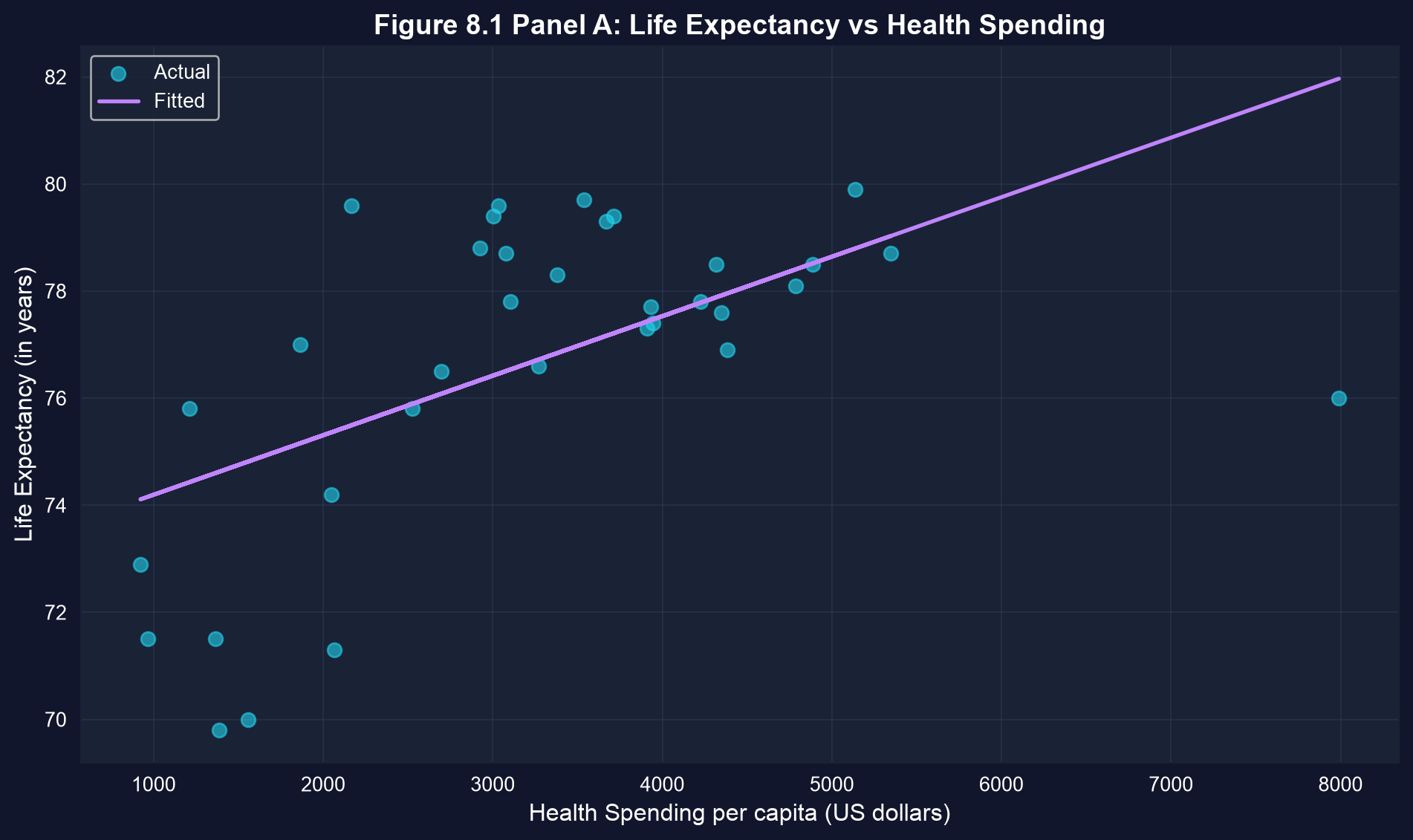
The estimated coefficient of 0.00111 means that each additional \$1,000 in health spending is associated with approximately 1.1 years of additional life expectancy. To put this in perspective:
- The difference between low-spending Chile (\$1,210/capita) and high-spending Norway (\$5,348/capita) is \$4,138
- This predicts a life expectancy difference of 4.6 years (4.138 × 1.11)
- Actual difference: 75.8 years (Chile) vs 78.7 years (Norway) = 2.9 years
**Statistical Significance:**
With classical (iid) standard errors the t-statistic is approximately 3.9 (p well below 0.001), strong evidence against the null hypothesis that health spending has no effect on life expectancy. With the heteroskedasticity-robust standard errors recommended above, the evidence weakens (robust t ≈ 2.4, p ≈ 0.02) but the relationship remains statistically significant at the 5% level.
**Important Caveats:**
1. This is correlation, not causation - richer countries may have both higher spending AND other factors that improve health
2. The relationship may not be linear across all spending levels
3. The U.S. is a notable outlier - spending \$7,990 per capita but achieving only 76.0 years (below prediction)
4. Other factors matter: diet, exercise, inequality, healthcare access, environmental quality
> **Key Concept 8.1: Economic vs. Statistical Significance**
>
> Economic vs. statistical significance in cross-country regressions. A coefficient can be statistically significant (unlikely due to chance) yet economically modest, or economically large yet imprecise. Always interpret both dimensions.
### Visualization: Life Expectancy vs Health Spending
The scatter plot below shows each country's health spending against male life expectancy, together with the fitted regression line. Look for the upward slope — and for the U.S., which lies well below the line.
```{python}
# Figure 8.1 Panel A - Life Expectancy
fig, ax = plt.subplots(figsize=(10, 6))
ax.scatter(data_health['hlthpc'], data_health['lifeexp'],
           alpha=0.6, s=50,  # alpha = transparency, s = marker size
           color='#22d3ee', label='Actual')
ax.plot(data_health['hlthpc'], model_lifeexp.predict(), color='#c084fc',
        linewidth=2, label='Fitted')
ax.set_xlabel('Health Spending per capita (US dollars)', fontsize=12)
ax.set_ylabel('Life Expectancy (in years)', fontsize=12)
ax.set_title('Figure 8.1 Panel A: Life Expectancy vs Health Spending',
             fontsize=14, fontweight='bold')
ax.legend()
ax.grid(True, alpha=0.3)
plt.tight_layout()
plt.show()

# Note: The U.S. has lower life expectancy than predicted by the model.
```
### Infant Mortality Regression
Next, we examine the relationship between health spending and infant mortality:
$$\text{Infmort} = \beta_1 + \beta_2 \times \text{Hlthpc} + u$$
We expect $\beta_2 < 0$ (higher spending reduces infant mortality).
```{python}
# Infant mortality regression
model_infmort = pf.feols('infmort ~ hlthpc', data=data_health)

# Key results
intercept_inf = model_infmort.coef()['Intercept']
slope_inf     = model_infmort.coef()['hlthpc']
r2_inf        = model_infmort._r2

print(f"Estimated equation: infmort = {intercept_inf:.2f} + ({slope_inf:.5f}) x hlthpc")
print(f"Slope: each additional $1,000 in spending is associated with {-slope_inf*1000:.2f} fewer infant deaths per 1,000 births")
print(f"R-squared: {r2_inf:.4f} ({r2_inf*100:.1f}% of variation explained)\n")

# Full regression output
model_infmort.summary()

# Robust standard errors
model_infmort_robust = pf.feols('infmort ~ hlthpc', data=data_health, vcov='HC1')

# Infant mortality regression (robust SE)
model_infmort_robust.summary()
```
### Interpreting the Infant Mortality Results
**Economic Significance:**
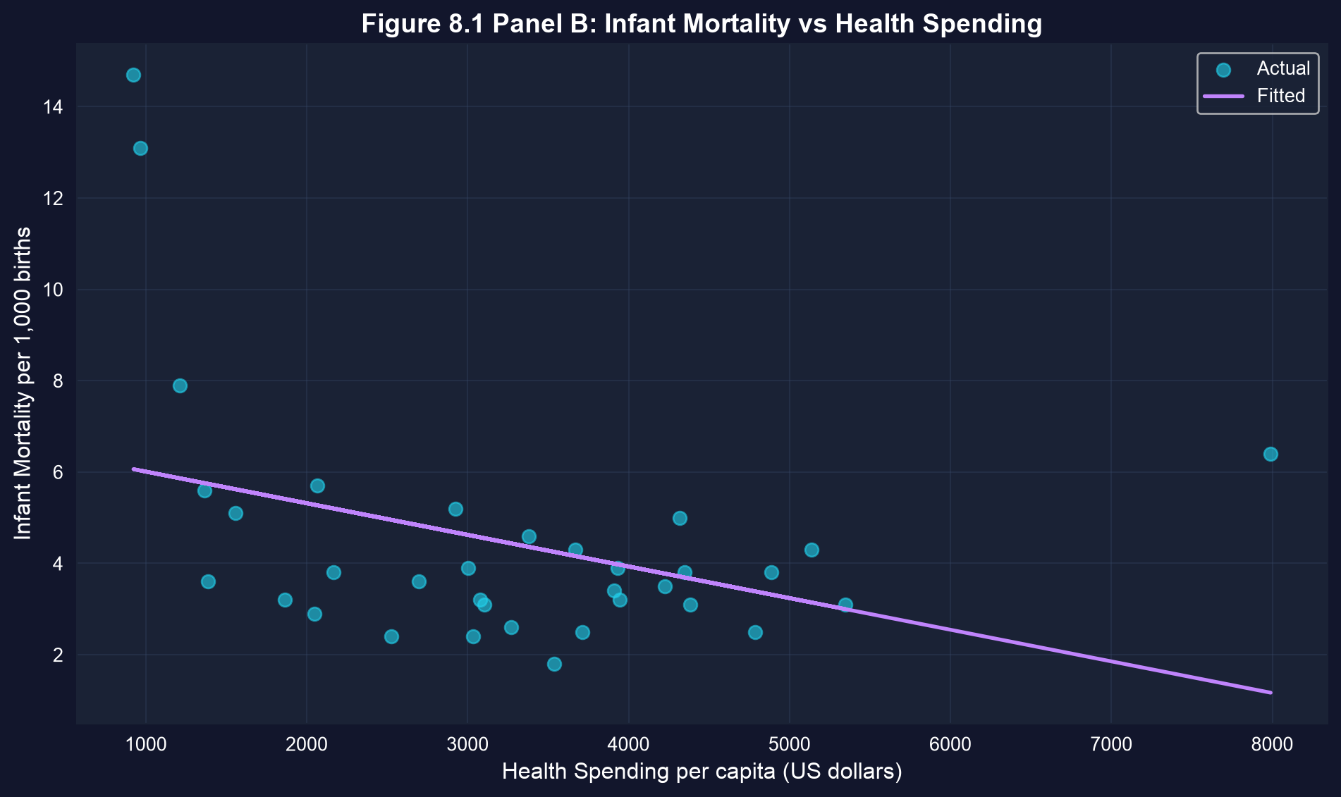
The estimated coefficient of approximately -0.00069 indicates that each additional \$1,000 in health spending is associated with a 0.69 decrease in infant deaths per 1,000 live births. While this may seem small, it's quite meaningful:
- A country increasing spending from \$2,000 to \$4,000 per capita would expect infant mortality to fall by 1.39 deaths per 1,000 births
- For a country with 100,000 births per year, this represents 139 fewer infant deaths annually
- The effect is economically significant in terms of human welfare
**Statistical Significance:**
With classical (iid) standard errors the negative relationship is statistically significant at the 5% level (t ≈ -2.3, p ≈ 0.03). But with the heteroskedasticity-robust standard errors that Key Concept 8.2 below calls essential, the standard error grows and the relationship is no longer significant at conventional levels (robust t ≈ -1.3, p ≈ 0.19). This is a cautionary example: a result that looks significant under classical assumptions can lose its significance once we allow for heteroskedasticity.
**The U.S. Anomaly:**
The United States again stands out as a major outlier:
- U.S. infant mortality: 6.4 deaths per 1,000 births
- Predicted based on spending (\$7,990): approximately 1.2 deaths per 1,000 births
- The U.S. has infant mortality rates closer to middle-income countries than to peer wealthy nations
- This suggests that *how* money is spent matters as much as *how much* is spent
**Model Limitations:**
The R² suggests health spending explains only about 14% of variation in infant mortality. Other important factors include:
- Quality of prenatal care and maternal health programs
- Income inequality and poverty rates
- Access to healthcare (insurance coverage)
- Cultural factors and health behaviors
> **Key Concept 8.2: Robust Standard Errors**
>
> Heteroskedasticity-robust standard errors adjust for non-constant error variance across observations. Cross-sectional data often exhibits heteroskedasticity (e.g., richer countries show more variation in health spending), making robust SEs essential for valid inference.
### Visualization: Infant Mortality vs Health Spending
The plot below shows infant mortality against health spending, with the fitted line. Look for the downward slope — and note how far the U.S. sits above the line.
```{python}
# Figure 8.1 Panel B - Infant Mortality
fig, ax = plt.subplots(figsize=(10, 6))
ax.scatter(data_health['hlthpc'], data_health['infmort'],
           alpha=0.6, s=50,  # alpha = transparency, s = marker size
           color='#22d3ee', label='Actual')
ax.plot(data_health['hlthpc'], model_infmort.predict(), color='#c084fc',
        linewidth=2, label='Fitted')
ax.set_xlabel('Health Spending per capita (US dollars)', fontsize=12)
ax.set_ylabel('Infant Mortality per 1,000 births', fontsize=12)
ax.set_title('Figure 8.1 Panel B: Infant Mortality vs Health Spending',
             fontsize=14, fontweight='bold')
ax.legend()
ax.grid(True, alpha=0.3)
plt.tight_layout()
plt.show()

# Note: The U.S. has much higher infant mortality than predicted.
```
Having examined how health spending affects outcomes, we now investigate what drives health spending itself. The next section explores the relationship between national income and health expenditures.
## 8.2 Health Expenditures Across Countries
Now we examine the determinants of health expenditures, focusing on the role of national income.
**Research question:** How does GDP per capita relate to health spending?
**Model:**
$$\text{Hlthpc} = \beta_1 + \beta_2 \times \text{Gdppc} + u$$
**Variables:**
- **Gdppc**: GDP per capita (US dollars)
- **Hlthpc**: Health expenditure per capita (US dollars)
**Key observation:** GDP per capita ranges from \$13,806 (Mexico) to \$82,901 (Luxembourg)
The summary statistics below quantify this variation in both GDP per capita and health spending.
```{python}
# 8.2 Health expenditures across countries

# Table 8.2: GDP and health spending summary
table82_vars = ['gdppc', 'hlthpc']
summary_gdp = data_health[table82_vars].describe().T
summary_gdp['range'] = summary_gdp['max'] - summary_gdp['min']
summary_gdp[['mean', 'std', 'min', 'max', 'range']]
```
### Health Expenditure Regression (All Countries)
We regress health spending on GDP per capita, first with default standard errors and then with robust ones. Compare the two summaries — the standard errors change noticeably, a sign of heteroskedasticity.
```{python}
# Health expenditure regression (all countries)
model_hlthpc = pf.feols('hlthpc ~ gdppc', data=data_health)

# Key results
intercept_hlth = model_hlthpc.coef()['Intercept']
slope_hlth     = model_hlthpc.coef()['gdppc']
r2_hlth        = model_hlthpc._r2

print(f"Estimated equation: hlthpc = {intercept_hlth:,.2f} + {slope_hlth:.4f} x gdppc")
print(f"R-squared: {r2_hlth:.4f} ({r2_hlth*100:.1f}% of variation explained)\n")

# Full regression output
model_hlthpc.summary()

# Robust standard errors
model_hlthpc_robust = pf.feols('hlthpc ~ gdppc', data=data_health, vcov='HC1')

# Health expenditure regression (robust SE)
model_hlthpc_robust.summary()
```
### Interpreting the Health Expenditure Results
**The GDP-Health Spending Relationship:**
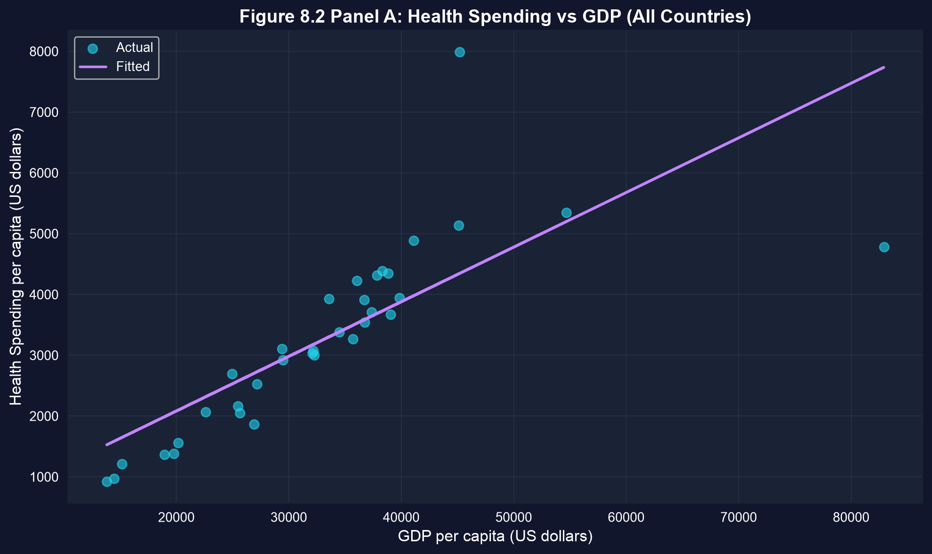
The coefficient of approximately 0.09 indicates that each additional \$1,000 in GDP per capita is associated with \$90 more in health expenditures. This relationship reveals important economic patterns:
**Income Elasticity of Health Spending:**
- At the mean GDP (\$33,054) and mean health spending (\$3,256):
- Elasticity ≈ (0.09 × 33,054) / 3,256 ≈ 0.9
- This suggests health spending rises roughly proportionally with income
- Health care appears to be a "normal good" (demand increases with income)
**Why Such Large Changes in Standard Errors?**
Notice how robust standard errors differ substantially from default standard errors:
- This indicates heteroskedasticity (non-constant error variance)
- Richer countries show more variation in health spending choices
- Luxembourg and the USA have enormous influence on the estimates
- Robust SEs adjust for this pattern and provide more reliable inference
- Even with robust standard errors, the GDP slope remains statistically significant (robust t ≈ 3.1, p ≈ 0.004), though the evidence is weaker than the default output suggests
**The Outlier Problem:**
Two countries drive much of the relationship:
1. **Luxembourg** (GDP: \$82,901, Health: \$4,786) - extremely wealthy, high spending
2. **United States** (GDP: \$45,192, Health: \$7,990) - exceptionally high health spending for its GDP level
These outliers suggest the relationship may not be stable across all countries.
> **Key Concept 8.3: Income Elasticity of Demand**
>
> Income elasticity of demand measures how spending changes with income. An elasticity near 1.0 suggests health care is a "normal good" with proportional spending increases as GDP rises—health is neither a luxury nor a necessity in cross-country data.
### Visualization: Health Spending vs GDP (All Countries)
The scatter plot below shows health spending against GDP per capita for all 34 countries, with the fitted line. Look for the two points that sit far from the rest — the USA and Luxembourg.
```{python}
# Figure 8.2 Panel A - All countries
fig, ax = plt.subplots(figsize=(10, 6))
ax.scatter(data_health['gdppc'], data_health['hlthpc'],
           alpha=0.6, s=50,  # alpha = transparency, s = marker size
           color='#22d3ee', label='Actual')
ax.plot(data_health['gdppc'], model_hlthpc.predict(), color='#c084fc',
        linewidth=2, label='Fitted')
ax.set_xlabel('GDP per capita (US dollars)', fontsize=12)
ax.set_ylabel('Health Spending per capita (US dollars)', fontsize=12)
ax.set_title('Figure 8.2 Panel A: Health Spending vs GDP (All Countries)',
             fontsize=14, fontweight='bold')
ax.legend()
ax.grid(True, alpha=0.3)
plt.tight_layout()
plt.show()

# The U.S. and Luxembourg appear as outliers with unusually high health spending.
```
### Robustness Check: Excluding USA and Luxembourg
To assess the influence of outliers, we re-estimate the model excluding the USA and Luxembourg.
```{python}
# Health expenditure regression (excluding USA and Luxembourg)

# Create subset excluding USA and Luxembourg
data_health_subset = data_health[(data_health['code'] != 'LUX') &
                                  (data_health['code'] != 'USA')]

print(f"Original sample size: {len(data_health)}")
print(f"Subset sample size: {len(data_health_subset)}")
print()

model_hlthpc_subset = pf.feols('hlthpc ~ gdppc', data=data_health_subset)

# Key results (excluding USA & Luxembourg)
intercept_sub = model_hlthpc_subset.coef()['Intercept']
slope_sub     = model_hlthpc_subset.coef()['gdppc']
r2_sub        = model_hlthpc_subset._r2

print(f"Estimated equation: hlthpc = {intercept_sub:,.2f} + {slope_sub:.4f} x gdppc")
print(f"R-squared: {r2_sub:.4f} ({r2_sub*100:.1f}% of variation explained)\n")

# Full regression output
model_hlthpc_subset.summary()

# Robust standard errors
model_hlthpc_subset_robust = pf.feols('hlthpc ~ gdppc', data=data_health_subset, vcov='HC1')

# Health expenditure regression (excluding USA & LUX, robust SE)
model_hlthpc_subset_robust.summary()
```
### Understanding the Impact of Outliers
**Dramatic Changes After Excluding USA and Luxembourg:**
The comparison reveals how sensitive regression results can be to outliers:
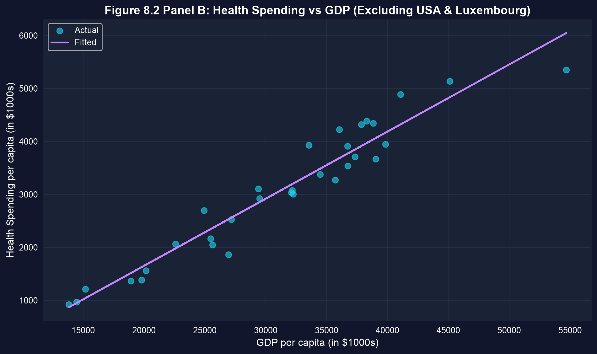
| Metric | Full Sample | Excluding USA & LUX | Change |
|--------|-------------|---------------------|--------|
| Slope | ~0.09 | ~0.13 | +41% |
| R² | ~0.60 | ~0.93 | +55% |
| Interpretation | Weak fit | Excellent fit | Transformed |
**What This Tells Us:**
1. **The USA is truly exceptional:** The U.S. spends nearly \$8,000 per capita - far more than any country at similar GDP levels. This reflects:
- Higher prices for medical services
- More intensive use of expensive technologies
- Administrative costs of a fragmented insurance system
- Less price regulation than in other OECD countries
2. **Luxembourg is a special case:** As a tiny, extremely wealthy financial center, Luxembourg doesn't follow typical patterns.
3. **The "true" relationship is stronger:** For the 32 typical OECD countries, the R² of 0.93 means GDP explains 93% of health spending variation. This is remarkably strong.
4. **Statistical lesson:** Always check for influential observations. A few extreme points can completely change your conclusions.
**Practical Implication:**
If you're advising a "typical" OECD country on expected health spending, the subset model provides more reliable guidance. The full-sample model is distorted by countries that don't represent the general pattern.
> **Key Concept 8.4: Outlier Detection and Influence**
>
> Outlier detection and influence. A few extreme observations can dramatically alter regression results. Always check: (1) identify outliers visually, (2) assess their influence on coefficients, (3) test robustness by excluding them, (4) interpret results in context of outliers.
### Visualization: Health Spending vs GDP (Excluding Outliers)
Re-plotting the 32 remaining countries shows how tightly they cluster around the fitted line once the two outliers are excluded.
```{python}
# Figure 8.2 Panel B - Excluding USA and Luxembourg
fig, ax = plt.subplots(figsize=(10, 6))
ax.scatter(data_health_subset['gdppc'], data_health_subset['hlthpc'],
           alpha=0.6, s=50,  # alpha = transparency, s = marker size
           color='#22d3ee', label='Actual')
ax.plot(data_health_subset['gdppc'], model_hlthpc_subset.predict(), color='#c084fc',
        linewidth=2, label='Fitted')
ax.set_xlabel('GDP per capita (in $1000s)', fontsize=12)
ax.set_ylabel('Health Spending per capita (in $1000s)', fontsize=12)
ax.set_title('Figure 8.2 Panel B: Health Spending vs GDP (Excluding USA & Luxembourg)',
             fontsize=14, fontweight='bold')
ax.legend()
ax.grid(True, alpha=0.3)
plt.tight_layout()
plt.show()

# Much stronger linear relationship when outliers are excluded.
```
Our health economics case studies revealed strong relationships but also highlighted outlier issues. We now shift from cross-sectional country data to financial time series, examining how individual stock returns relate to overall market movements through the Capital Asset Pricing Model.
## 8.3 Capital Asset Pricing Model (CAPM)
Our third case study applies regression to financial data using the Capital Asset Pricing Model.
**Theory:**
The CAPM relates individual stock returns to overall market returns:
$$E[R_A - R_F] = \beta_A \times E[R_M - R_F]$$
where:
- $R_A$ = return on asset A (e.g., Coca-Cola stock)
- $R_F$ = risk-free rate (1-month U.S. Treasury bill)
- $R_M$ = market return (value-weighted return on all stocks)
- $\beta_A$ = systematic risk ("beta") of asset A
**Empirical model:**
$$R_A - R_F = \alpha_A + \beta_A (R_M - R_F) + u$$
**Interpretation:**
- $\beta_A$ = systematic risk (average across market is 1.0)
- $\beta > 1$: Stock is riskier than market (growth stock)
- $\beta < 1$: Stock is less risky (value stock)
- $\beta \approx 0$: Stock moves independently of market
- $\alpha_A$ = excess return ("alpha") after adjusting for risk
- Pure CAPM theory predicts $\alpha = 0$
**Dataset:** Monthly data from May 1983 to October 2012 (354 observations)
- Returns on Coca-Cola (RKO), Target (RTGT), Walmart (RWMT)
- Market return and risk-free rate
```{python}
# 8.3 CAPM model

# Read in the CAPM data
data_capm = pd.read_stata(GITHUB_DATA_URL + 'AED_CAPM.DTA')

# Data summary
display(data_capm.describe())

# First few observations
data_capm[['date', 'rm', 'rf', 'rko', 'rm_rf', 'rko_rf']].head()
```
### Summary Statistics for CAPM Variables
Before estimating the CAPM, we summarize the monthly return series. Compare the standard deviations: the individual stocks are clearly more volatile than the market.
```{python}
# Table 8.3: CAPM variables summary
table83_vars = ['rm', 'rf', 'rko', 'rtgt', 'rwmt', 'rm_rf',
                'rko_rf', 'rtgt_rf', 'rwmt_rf']
summary_capm = data_capm[table83_vars].describe().T
display(summary_capm[['mean', 'std', 'min', 'max']])

print("\nKey observations:")
print(f"  - Market excess return averages {data_capm['rm_rf'].mean():.4f} ({data_capm['rm_rf'].mean()*100:.2f}% per month)")
print(f"  - Coca-Cola excess return averages {data_capm['rko_rf'].mean():.4f} ({data_capm['rko_rf'].mean()*100:.2f}% per month)")
print(f"  - Stock returns are much more volatile than market returns")
```
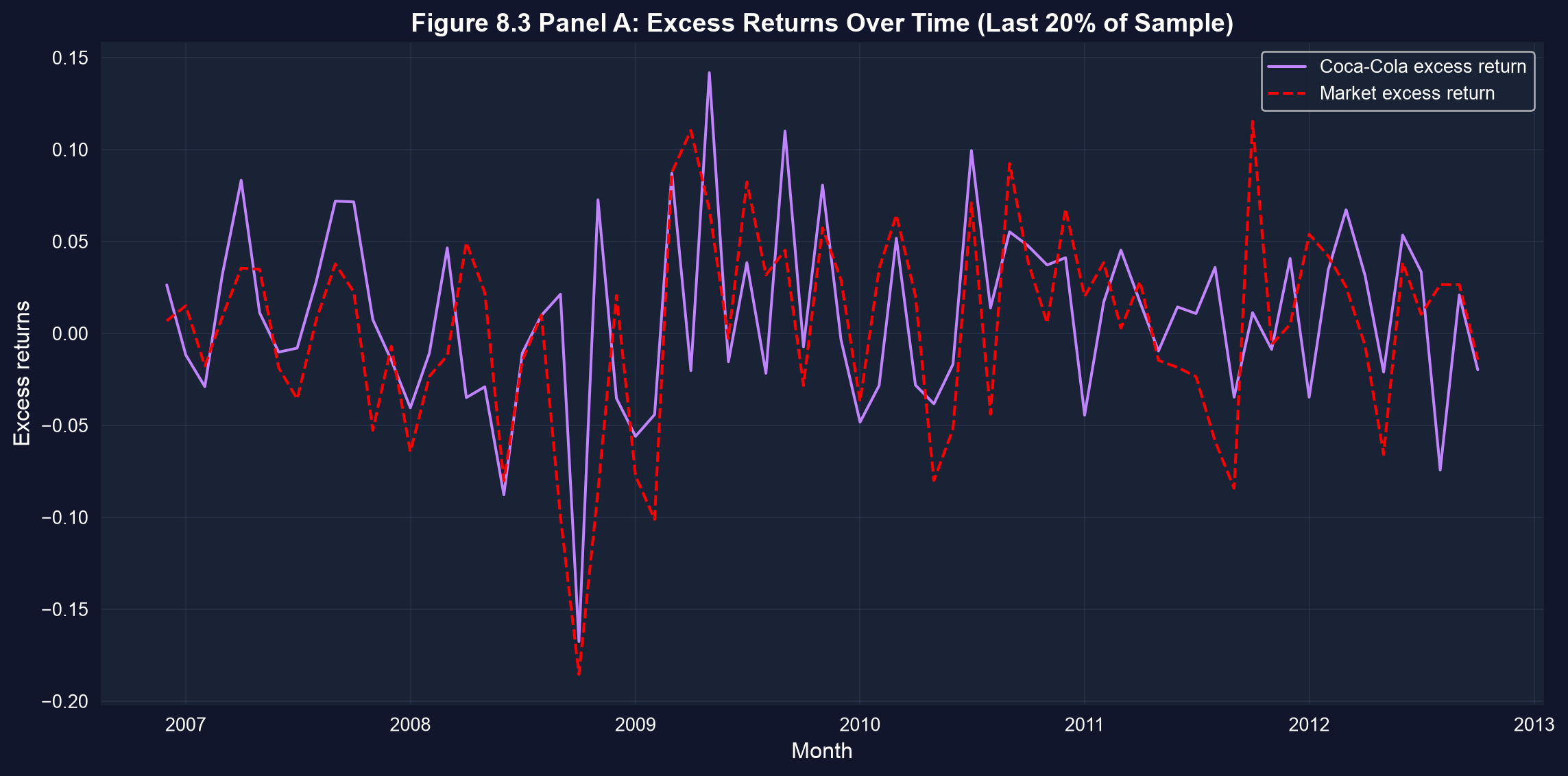
### Visualization: Time Series of Excess Returns
The plot below traces Coca-Cola's and the market's excess returns over the most recent fifth of the sample. Notice how the stock's line swings more widely than the market's.
```{python}
# Figure 8.3 Panel A - Time series plot (last 20% of data for readability)
cutoff_index = int(len(data_capm) * 0.8)
data_capm_recent = data_capm.iloc[cutoff_index:]

fig, ax = plt.subplots(figsize=(12, 6))
ax.plot(data_capm_recent['date'], data_capm_recent['rko_rf'],
        linewidth=1.5, label='Coca-Cola excess return', color='#c084fc')
ax.plot(data_capm_recent['date'], data_capm_recent['rm_rf'],
        linewidth=1.5, linestyle='--', label='Market excess return', color='red')
ax.set_xlabel('Month', fontsize=12)
ax.set_ylabel('Excess returns', fontsize=12)
ax.set_title('Figure 8.3 Panel A: Excess Returns Over Time (Last 20% of Sample)',
             fontsize=14, fontweight='bold')
ax.legend()
ax.grid(True, alpha=0.3)
plt.tight_layout()
plt.show()

# Individual stock returns fluctuate more than the overall market.
```
### CAPM Regression for Coca-Cola
We now estimate the CAPM regression of Coca-Cola's excess return on the market's excess return. The slope is Coca-Cola's beta — check whether it is above or below 1 in the output.
```{python}
# CAPM regression: Coca-Cola
model_capm = pf.feols('rko_rf ~ rm_rf', data=data_capm)

# Key results
alpha = model_capm.coef()['Intercept']
beta = model_capm.coef()['rm_rf']
r2_capm = model_capm._r2

print(f"Estimated equation: rko_rf = {alpha:.4f} + {beta:.4f} x rm_rf")
print(f"Beta (systematic risk): {beta:.4f} — Coca-Cola is a defensive stock (beta < 1)")
print(f"R-squared: {r2_capm:.4f} ({r2_capm*100:.1f}% of return variation explained by market)\n")

# Full regression output
model_capm.summary()
```
### CAPM Results with Robust Standard Errors
```{python}
# CAPM regression: Coca-Cola (robust SE)
model_capm_robust = pf.feols('rko_rf ~ rm_rf', data=data_capm, vcov='HC1')
model_capm_robust.summary()
```
### Interpreting the CAPM Beta for Coca-Cola
**What Beta = 0.61 Means:**
The estimated beta of 0.61 reveals Coca-Cola's risk profile:
1. **Lower systematic risk than the market:**
- Beta < 1 means Coca-Cola is a "defensive" or "value" stock
- When the market rises 10%, Coca-Cola typically rises only 6.1%
- When the market falls 10%, Coca-Cola typically falls only 6.1%
- This makes it attractive to risk-averse investors
2. **Why is Coca-Cola low-beta?**
- Stable demand for consumer staples (people drink Coke in good times and bad)
- Strong brand loyalty reduces volatility
- Diversified global operations
- Predictable cash flows
- Less sensitive to economic cycles than growth stocks
3. **Statistical precision:**
- The t-statistic of ~9.4 provides overwhelming evidence that beta ≠ 0
- Coca-Cola returns clearly co-move with the market
- The relationship is one of the strongest we've seen in this chapter
**The Alpha "Puzzle":**
The estimated alpha of 0.0068 (0.68% per month, or ~8.2% annually) is statistically significant:
- Pure CAPM theory predicts alpha should equal zero (no excess risk-adjusted returns)
- Yet we reject H₀: α = 0 at conventional significance levels
- This suggests either:
- CAPM is misspecified (missing risk factors)
- Coca-Cola generated genuine excess returns during 1983-2012
- Statistical artifact from data mining
**Investment Implications:**
- Coca-Cola is suitable for conservative portfolios seeking market exposure with lower volatility
- The low beta means lower expected returns in bull markets, but better downside protection in bear markets
- Institutional investors often use low-beta stocks to reduce portfolio risk while maintaining equity exposure
> **Key Concept 8.5: Systematic Risk and Beta**
>
> Systematic risk (beta) measures how an asset's returns co-move with the overall market. Beta < 1 indicates a "defensive" stock (less volatile than market), while beta > 1 indicates a "growth" stock (amplifies market movements). Only systematic risk is priced in efficient markets.
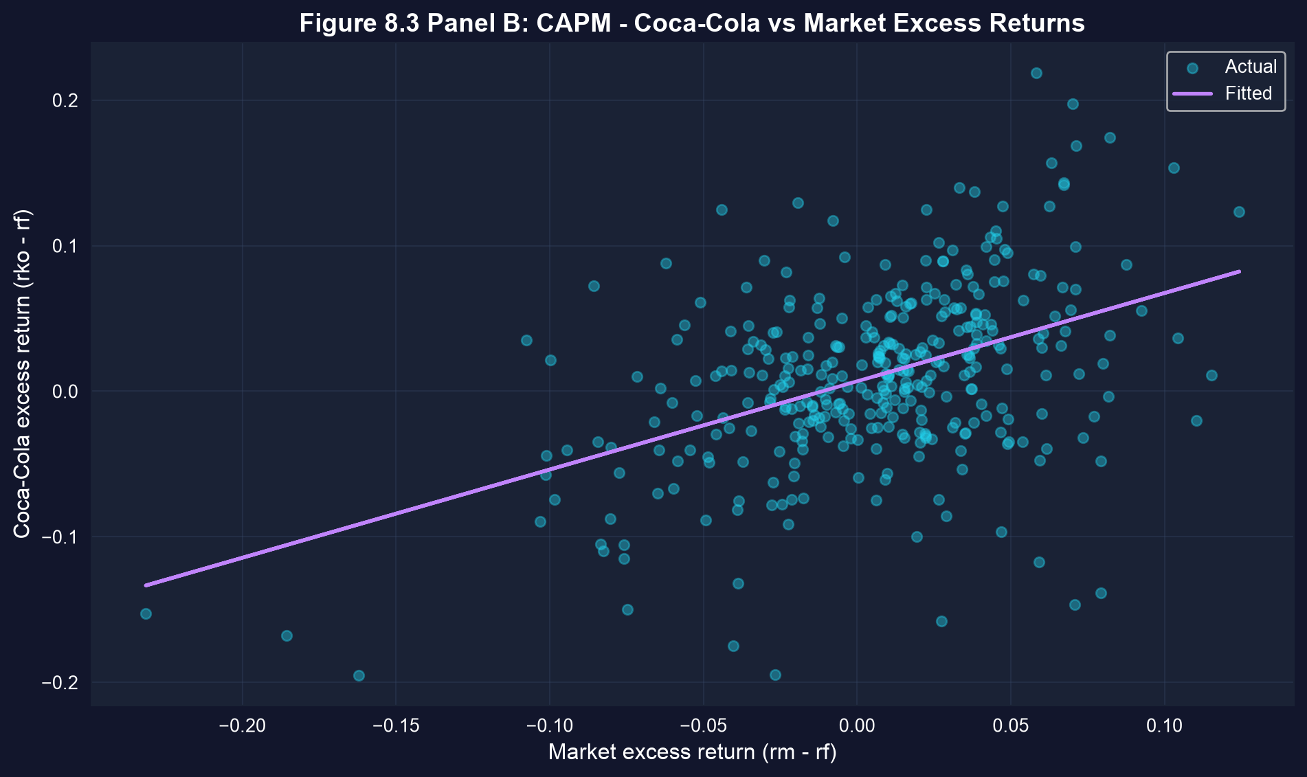
### Visualization: CAPM Scatter Plot
The scatter plot below shows every monthly observation with the fitted CAPM line. Note the wide dispersion around the line — most of Coca-Cola's month-to-month variation is firm-specific rather than market-driven.
```{python}
# Figure 8.3 Panel B - CAPM Scatter Plot
fig, ax = plt.subplots(figsize=(10, 6))
ax.scatter(data_capm['rm_rf'], data_capm['rko_rf'],
           alpha=0.4, s=30,  # alpha = transparency, s = marker size
           color='#22d3ee', label='Actual')
ax.plot(data_capm['rm_rf'], model_capm.predict(), color='#c084fc',
        linewidth=2, label='Fitted')
ax.set_xlabel('Market excess return (rm - rf)', fontsize=12)
ax.set_ylabel('Coca-Cola excess return (rko - rf)', fontsize=12)
ax.set_title('Figure 8.3 Panel B: CAPM - Coca-Cola vs Market Excess Returns',
             fontsize=14, fontweight='bold')
ax.legend()
ax.grid(True, alpha=0.3)
plt.tight_layout()
plt.show()

print(f"Beta (slope) = {model_capm.coef()['rm_rf']:.4f}")
# The slope less than 1 confirms Coca-Cola is a 'defensive' stock.
# Each 1% increase in market return -> ~0.6% increase in Coca-Cola return.
```
### Understanding the CAPM Scatter Plot
**Key Visual Insights:**
1. **Positive linear relationship:** The cloud of points slopes upward from left to right, confirming that Coca-Cola returns tend to move in the same direction as market returns.
2. **Scatter around the line:** The substantial dispersion around the regression line reflects:
- Idiosyncratic risk (firm-specific factors): management decisions, product launches, competitive pressures
- The R² ≈ 0.20 means the market explains only 20% of Coca-Cola's return variation
- The remaining 80% is diversifiable risk that disappears in a portfolio
3. **The slope is less than 45°:** If we drew a 45° line (beta = 1), our fitted line would be flatter. This visually confirms beta < 1.
4. **Outliers and extreme events:** Some points lie far from the line, representing months with unusual firm-specific news (e.g., earnings surprises, regulatory changes, management changes).
**Comparison to Theory:**
- In a pure CAPM world, the intercept (alpha) would be exactly zero and the line would pass through the origin
- Our line has a positive intercept, suggesting Coca-Cola earned excess returns beyond what CAPM predicts
- This is common in empirical finance - CAPM is a useful model but not a perfect description of reality
**Time Series Considerations:**
- CAPM assumes returns are independent over time (no autocorrelation)
- With monthly data spanning nearly 30 years, we should ideally check for time-varying beta
- Some periods (recessions) may show different beta than others (expansions)
- More sophisticated models (e.g., conditional CAPM) could account for this
> **Key Concept 8.6: R-Squared in CAPM**
>
> R² in the CAPM context. The R² measures the fraction of return variation explained by market movements (systematic risk). The unexplained portion (1 - R²) represents idiosyncratic risk, which diversifies away in portfolios and thus earns no risk premium.
The CAPM demonstrated how financial returns co-move with market-wide factors. Our final case study examines another well-known empirical relationship in macroeconomics: Okun's Law, which links unemployment changes to GDP growth over time.
## 8.4 Output and Unemployment in the U.S. (Okun's Law)
Our final case study examines a fundamental macroeconomic relationship known as Okun's Law.
**Okun's Law (1962):**
Each percentage point increase in the unemployment rate is associated with approximately a two percentage point decrease in GDP growth.
**Empirical model:**
$$\text{Growth} = \beta_1 + \beta_2 \times \text{URATEchange} + u$$
where:
- **Growth**: Annual percentage growth in real GDP
- **URATEchange**: Annual change in unemployment rate (percentage points)
**Hypothesis:** Okun's law suggests $\beta_2 = -2.0$
**Dataset:** Annual U.S. data from 1961 to 2019 (59 observations)
- Real GDP growth
- Unemployment rate for civilian population aged 16 and older
```{python}
# 8.4 Output and unemployment in the U.S.

# Read in the GDP-Unemployment data
data_gdp = pd.read_stata(GITHUB_DATA_URL + 'AED_GDPUNEMPLOY.DTA')

# Data summary
display(data_gdp.describe())

# First few observations
data_gdp[['year', 'rgdpgrowth', 'uratechange']].head(10)
```
### Summary Statistics
We first summarize the two series. GDP growth averages about 3% per year, while the average change in unemployment is close to zero.
```{python}
# Table 8.4: GDP growth and unemployment change summary
table84_vars = ['rgdpgrowth', 'uratechange']
summary_gdp_tbl = data_gdp[table84_vars].describe().T
display(summary_gdp_tbl[['mean', 'std', 'min', 'max']])

print("\nKey observations:")
print(f"  - Average GDP growth: {data_gdp['rgdpgrowth'].mean():.2f}%")
print(f"  - Average unemployment change: {data_gdp['uratechange'].mean():.3f} percentage points")
print(f"  - Sample period includes major recessions (1982, 2008-2009)")
```
### Okun's Law Regression
We estimate Okun's Law by regressing real GDP growth on the change in the unemployment rate. Compare the estimated slope in the output with Okun's benchmark of -2.0.
```{python}
# Okun's law regression
model_okun = pf.feols('rgdpgrowth ~ uratechange', data=data_gdp)

# Key results
intercept_okun = model_okun.coef()['Intercept']
slope_okun = model_okun.coef()['uratechange']
r2_okun = model_okun._r2

print(f"Estimated equation: GDP_growth = {intercept_okun:.2f} + ({slope_okun:.2f}) x URATEchange")
print(f"R-squared: {r2_okun:.4f} ({r2_okun*100:.1f}% of variation explained)\n")

# Full regression output
model_okun.summary()
```
### Okun's Law with Robust Standard Errors
```{python}
# Okun's law regression (robust SE)
model_okun_robust = pf.feols('rgdpgrowth ~ uratechange', data=data_gdp, vcov='HC1')
model_okun_robust.summary()
```
### Interpreting Okun's Law Results
**The Estimated Relationship:**
Our coefficient of -1.59 is reasonably close to Okun's original -2.0, but statistically different. What does this mean?
**Economic Interpretation:**
- A 1 percentage point increase in unemployment → 1.59 percentage point decrease in GDP growth
- This is slightly weaker than Okun's original finding, but still substantial
- Example: If unemployment rises from 5% to 6% (+1 point), GDP growth falls from 3% to 1.41%
**Why Not Exactly -2.0?**
Several factors could explain the difference:
1. **Time period:** Okun's original study used 1947-1960 data. Our sample (1961-2019) spans a different economic era with:
- Different labor market institutions
- Shift from manufacturing to services
- Changes in productivity growth patterns
- Greater labor force participation volatility
2. **Structural changes in the economy:**
- The relationship between output and employment may have weakened
- More flexible labor markets may dampen the GDP-unemployment link
- Changes in the natural rate of unemployment
3. **Sample includes major crises:**
- 2008-2009 financial crisis with unprecedented unemployment spike
- 1982 recession with very high unemployment
- These may have different dynamics than typical recessions
**Testing β = -2.0:**
The t-statistic of ~2.4 indicates we reject Okun's exact -2.0 at the 5% level. However:
- The 95% confidence interval, roughly [-1.94, -1.24], excludes -2.0 — consistent with the rejection — though its lower bound is not far from -2.0
- The difference (-1.59 vs -2.0) is economically modest
- For practical policy purposes, the relationship is "close enough" to Okun's law
**Model Fit:**
R² = 0.59 means unemployment changes explain 59% of GDP growth variation:
- This is quite high for a bivariate macroeconomic relationship
- The remaining 41% reflects other factors: productivity shocks, trade, investment, government policy, monetary shocks
> **Key Concept 8.7: Okun's Law**
>
> Okun's Law as an empirical regularity. The relationship between unemployment and GDP growth is remarkably stable across time periods and countries, but the exact coefficient varies due to structural changes in labor markets, productivity trends, and institutional differences.
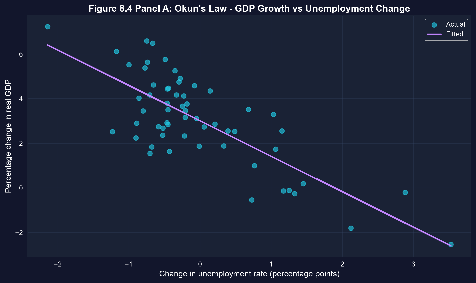
### Visualization: Okun's Law Scatter Plot
In the scatter plot below, each point is one year of U.S. data and the fitted line traces Okun's Law. Look for the recession years far from the main cluster, where unemployment jumped and growth collapsed.
```{python}
# Figure 8.4 Panel A - Okun's Law Scatter Plot
fig, ax = plt.subplots(figsize=(10, 6))
ax.scatter(data_gdp['uratechange'], data_gdp['rgdpgrowth'],
           alpha=0.6, s=50,  # alpha = transparency, s = marker size
           color='#22d3ee', label='Actual')
ax.plot(data_gdp['uratechange'], model_okun.predict(), color='#c084fc',
        linewidth=2, label='Fitted')
ax.set_xlabel('Change in unemployment rate (percentage points)', fontsize=12)
ax.set_ylabel('Percentage change in real GDP', fontsize=12)
ax.set_title('Figure 8.4 Panel A: Okun\'s Law - GDP Growth vs Unemployment Change',
             fontsize=14, fontweight='bold')
ax.legend()
ax.grid(True, alpha=0.3)
plt.tight_layout()
plt.show()

# Each point represents one year of U.S. macroeconomic data (1961-2019).
# The negative slope confirms Okun's Law: rising unemployment -> falling GDP.
```
### Understanding the Okun's Law Scatter Plot
**Visual Pattern Analysis:**
1. **Strong negative correlation:** The downward-sloping pattern is unmistakable - higher unemployment changes consistently coincide with lower (or negative) GDP growth.
2. **Clustering around the origin:** Most observations lie near the center, representing normal economic times with modest changes in both unemployment and GDP. This is typical of stable economic periods.
3. **Outliers reveal recessions:** Points in the upper-left quadrant represent major recessions:
- **2009**: Unemployment rose ~3.5 percentage points, GDP fell ~2.5%
- **1982**: Unemployment rose ~2.1 points, GDP fell ~1.8%
- **2020**: (if included) would show extreme values from COVID-19 pandemic
4. **Asymmetry:** The scatter isn't perfectly symmetric:
- Large unemployment increases (recessions) tend to cluster together
- Unemployment decreases (recoveries) are more gradual and dispersed
- This reflects that recessions happen quickly, but recoveries take time
5. **The fitted line:** The slope of -1.59 captures the average relationship, but individual points can deviate substantially:
- Some recessions are deeper than predicted
- Some recoveries are stronger than predicted
- The 2008-2009 financial crisis shows a flatter relationship (weak recovery)
**Policy Implications:**
This visualization demonstrates why policymakers monitor unemployment so closely:
- Rising unemployment is a reliable signal of falling GDP
- The relationship is strong enough to be useful for forecasting
- But the scatter reminds us that the relationship isn't deterministic - other factors matter too
**Data Quality Note:**
Unlike cross-sectional health data, these are time series observations that may exhibit:
- Serial correlation (one year's growth affects the next)
- Structural breaks (relationship changes over time)
- Heteroskedasticity (variance changes across different economic regimes)
More advanced time series methods could improve on this simple OLS regression.
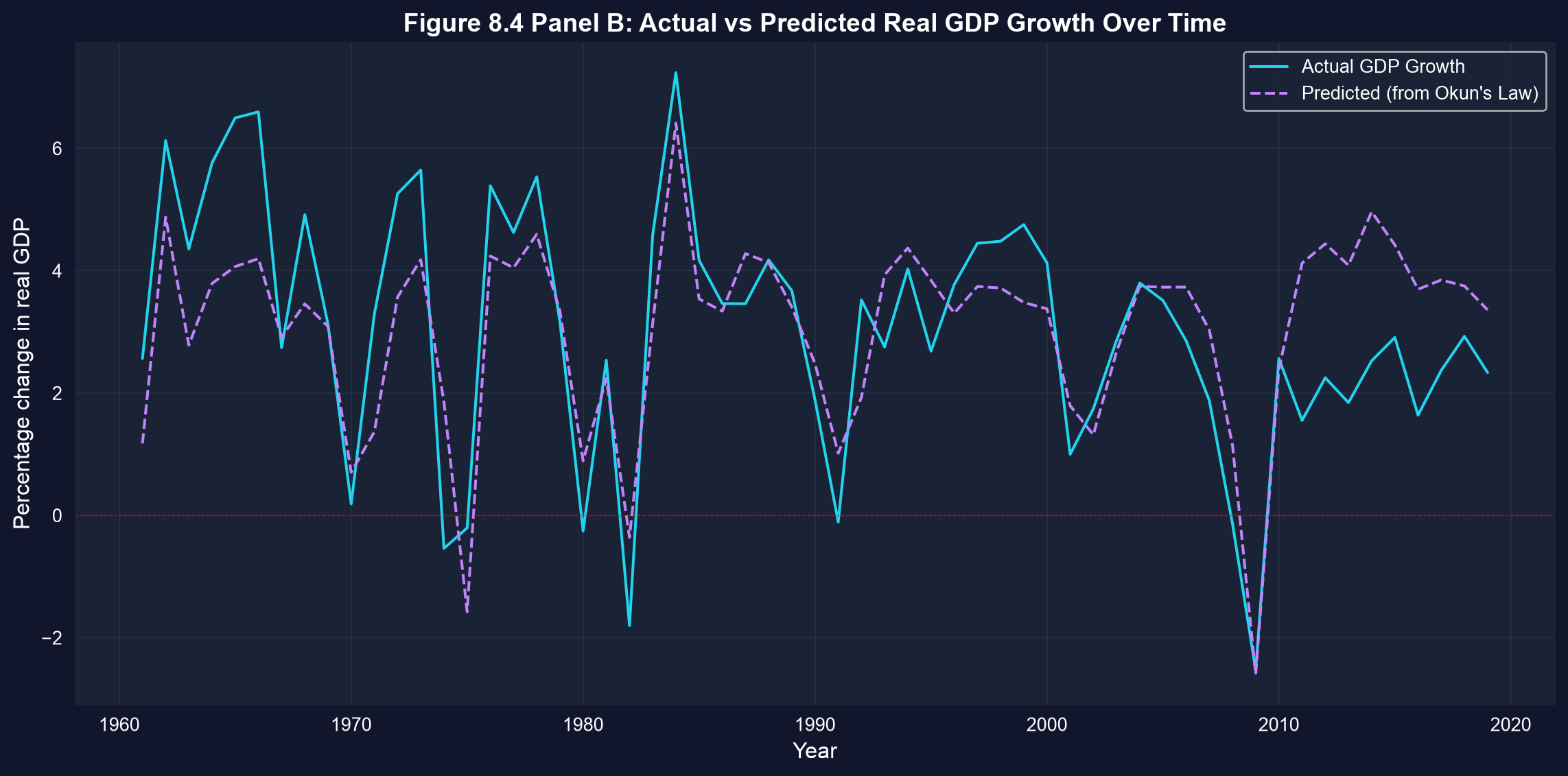
### Visualization: Time Series of Actual vs Predicted GDP Growth
Finally, we plot actual GDP growth alongside the values predicted from unemployment changes alone. Watch how closely the two lines track each other before 2008 — and how they diverge afterward.
```{python}
# Figure 8.4 Panel B - Time Series of Actual vs Predicted GDP Growth
fig, ax = plt.subplots(figsize=(12, 6))
ax.plot(data_gdp['year'], data_gdp['rgdpgrowth'], linewidth=1.5,
        label='Actual GDP Growth', color='#22d3ee')
ax.plot(data_gdp['year'], model_okun.predict(), linewidth=1.5, linestyle='--',
        label='Predicted (from Okun\'s Law)', color='#c084fc')
ax.axhline(y=0, color='red', linestyle=':', linewidth=1, alpha=0.5)
ax.set_xlabel('Year', fontsize=12)
ax.set_ylabel('Percentage change in real GDP', fontsize=12)
ax.set_title('Figure 8.4 Panel B: Actual vs Predicted Real GDP Growth Over Time',
             fontsize=14, fontweight='bold')
ax.legend()
ax.grid(True, alpha=0.3)
plt.tight_layout()
plt.show()

# Major recessions visible: 1982, 1991, 2001, 2008-2009
# Note: After 2010 actual GDP growth falls below Okun's Law predictions (unemployment fell faster than GDP grew).
```
### Analyzing the Time Series of Actual vs. Predicted GDP Growth
**What This Graph Reveals:**
1. **Model tracks major recessions well:**
- The predicted line (dashed) captures the timing and direction of major downturns
- 1982, 1991, 2001, 2008-2009 recessions are all identified by the model
- This validates Okun's Law as a useful empirical relationship
2. **Systematic prediction errors in the 2010s:**
- After 2010, actual GDP growth (cyan line) consistently falls *below* the growth predicted from unemployment changes (9 of the 10 years from 2010 to 2019)
- Unemployment fell faster than the modest GDP growth would imply, so Okun's Law over-predicts growth in this period
- Possible explanations:
- Declining labor force participation: the falling unemployment rate overstated the true improvement in the labor market
- Weak productivity growth — employment rose but output per worker stagnated
- Structural changes in labor markets after the financial crisis
- A slower, less capital-intensive recovery than in past cycles
3. **Pre-2008 fit is excellent:**
- Before the financial crisis, actual and predicted values track each other closely
- This suggests Okun's Law held remarkably well for 1961-2007
- The post-2008 divergence may represent a structural break
4. **Volatility patterns:**
- GDP growth is more volatile than predicted by unemployment alone
- Large spikes (both positive and negative) aren't fully captured
- This reflects the 41% of variation (1 - R²) unexplained by unemployment changes
**Economic Insights:**
- **2008-2009 Crisis:** The model slightly over-predicts the severity of the 2009 GDP collapse — actual growth (about -2.5%) was marginally better than the -2.6% the unemployment spike implied, so the crisis fits the historical relationship reasonably well
- **Recovery paradox:** As unemployment fell steadily after 2010, Okun's Law predicted a strong recovery (roughly 4% growth), yet actual GDP growth was more modest (about 2 to 2.5%). Employment recovered faster than output, challenging conventional wisdom about the output-employment relationship.
- **Policy relevance:** Central banks and fiscal authorities use Okun's Law for forecasting, but this graph shows the relationship isn't immutable - structural changes can alter the coefficients over time.
**Methodological Note:**
This type of time series plot is more informative than just reporting R² because it reveals:
- When the model works well (1980s-1990s)
- When it breaks down (2010s)
- Whether errors are random or systematic
- The presence of potential structural breaks that might warrant separate subperiod analysis
> **Key Concept 8.8: Structural Breaks**
>
> Structural breaks in time series relationships. Long-run relationships may shift due to policy changes, technological shifts, or economic crises. Visual inspection of actual vs. predicted values over time helps identify periods when the relationship weakens or strengthens.
## Key Takeaways
**Case Study Applications:**
- Health spending and life expectancy: +$1,000 spending → +1.11 years life expectancy
- Health spending and infant mortality: +$1,000 spending → -0.69 infant deaths per 1,000 births
- GDP and health spending: +$1,000 GDP → +$90 health expenditures (elasticity ≈ 0.9)
- CAPM beta for Coca-Cola: 0.61 (defensive stock, less risky than market)
- Okun's Law: +1 percentage point unemployment → -1.59 percentage points GDP growth
**Statistical Methods Applied:**
- Bivariate regression estimation (OLS)
- Heteroskedasticity-robust standard errors (HC1)
- Hypothesis testing for specific parameter values (t-tests)
- Confidence interval construction and interpretation
- Outlier detection and influence assessment
- Economic vs. statistical significance comparison
**Key Economic Insights:**
- U.S. health outcomes worse than predicted by spending levels
- USA and Luxembourg are outliers with exceptionally high health spending
- Excluding outliers transforms health-GDP relationship (R² 0.60 → 0.93)
- Coca-Cola's low beta reflects stable consumer demand across business cycles
- Okun's Law coefficient (-1.59) close to original -2.0 but statistically different
- Post-2008 "jobless recovery" weakened traditional Okun relationship
**Technical Skills Mastered:**
- Applying regression to cross-sectional, financial, and time series data
- Using robust standard errors for valid inference
- Testing economic hypotheses beyond β = 0
- Identifying and handling influential observations
- Interpreting coefficients in economic context (policy implications)
- Creating publication-quality visualizations (scatter plots, time series)
**Python Tools:**
- `pandas`: Data manipulation, summary statistics, subsetting
- `pyfixest.feols()`: Regression estimation with built-in robust SEs
- `pf.feols(..., vcov='HC1')`: Heteroskedasticity-robust standard errors
- `matplotlib` & `seaborn`: Professional visualizations
- `scipy.stats`: Statistical distributions
**Data Types Covered:**
- Cross-sectional: OECD health data (34 countries)
- Financial time series: Monthly stock returns (1983-2012)
- Macroeconomic time series: Annual GDP and unemployment (1961-2019)
- Multi-domain applications: Health, finance, macroeconomics
**Python Libraries and Code:**
This single code block reproduces the core workflow of Chapter 8. It is self-contained — copy it into an empty notebook and run it to review the complete pipeline from health regressions to CAPM betas and Okun's Law.
```python
# =============================================================================
# CHAPTER 8 CHEAT SHEET: Case Studies for Bivariate Regression
# =============================================================================

# --- Libraries ---
import pandas as pd                       # data loading and manipulation
import matplotlib.pyplot as plt           # creating plots and visualizations
import pyfixest as pf                     # fast estimation with robust SEs

# =============================================================================
# STEP 1: Load OECD health data from a URL
# =============================================================================
# pd.read_stata() reads Stata .dta files — this dataset covers 34 OECD countries
url_health = "https://raw.githubusercontent.com/quarcs-lab/data-open/master/AED/AED_HEALTH2009.DTA"
data_health = pd.read_stata(url_health)

print(f"Health dataset: {data_health.shape[0]} countries, {data_health.shape[1]} variables")

# =============================================================================
# STEP 2: Descriptive statistics — summarize before modeling
# =============================================================================
# .describe() gives mean, std, min, quartiles, max for each variable
print(data_health[['hlthpc', 'lifeexp', 'infmort', 'gdppc']].describe().round(2))

# =============================================================================
# STEP 3: Health outcomes regression with robust standard errors
# =============================================================================
# Does higher health spending improve life expectancy?
model_life = pf.feols('lifeexp ~ hlthpc', data=data_health)

slope_life = model_life.coef()['hlthpc']
r2_life    = model_life._r2

print(f"Life expectancy: slope = {slope_life:.5f}, R² = {r2_life:.4f}")
print(f"Each extra $1,000 in spending → {slope_life*1000:.2f} more years of life expectancy")

# Robust standard errors adjust for non-constant error variance (heteroskedasticity)
model_life_robust = pf.feols('lifeexp ~ hlthpc', data=data_health, vcov='HC1')
model_life_robust.summary()

# =============================================================================
# STEP 4: Health spending vs GDP — income elasticity
# =============================================================================
# How much of health spending is driven by national income?
model_gdp = pf.feols('hlthpc ~ gdppc', data=data_health)

slope_gdp = model_gdp.coef()['gdppc']
r2_gdp    = model_gdp._r2

# Income elasticity at the mean: (slope × mean_x) / mean_y
mean_gdp  = data_health['gdppc'].mean()
mean_hlth = data_health['hlthpc'].mean()
elasticity = (slope_gdp * mean_gdp) / mean_hlth

print(f"Health spending on GDP: slope = {slope_gdp:.4f}, R² = {r2_gdp:.4f}")
print(f"Income elasticity at the mean: {elasticity:.2f} (near 1 → normal good)")

# =============================================================================
# STEP 5: Outlier robustness — excluding USA and Luxembourg
# =============================================================================
# Two countries drive much of the model's "misfit" — test robustness by excluding them
data_subset = data_health[(data_health['code'] != 'USA') &
                          (data_health['code'] != 'LUX')]

model_subset = pf.feols('hlthpc ~ gdppc', data=data_subset)

print(f"\nAll 34 countries:  slope = {slope_gdp:.4f}, R² = {r2_gdp:.4f}")
print(f"Excluding USA/LUX: slope = {model_subset.coef()['gdppc']:.4f}, R² = {model_subset._r2:.4f}")
print("Removing 2 of 34 countries transforms R² — always check for influential observations!")

fig, axes = plt.subplots(1, 2, figsize=(14, 5))
for ax, df, mdl, title in zip(
        axes,
        [data_health, data_subset],
        [model_gdp, model_subset],
        ['All 34 Countries', 'Excluding USA & Luxembourg']):
    ax.scatter(df['gdppc'], df['hlthpc'], s=50, alpha=0.7)
    ax.plot(df['gdppc'], mdl.predict(), color='red', linewidth=2)
    ax.set_xlabel('GDP per capita ($)')
    ax.set_ylabel('Health spending per capita ($)')
    ax.set_title(f'{title}  (R² = {mdl._r2:.2f})')
    ax.grid(True, alpha=0.3)
plt.tight_layout()
plt.show()

# =============================================================================
# STEP 6: CAPM — estimating Coca-Cola's beta (systematic risk)
# =============================================================================
# Beta measures how a stock's excess return co-moves with the market excess return
url_capm = "https://raw.githubusercontent.com/quarcs-lab/data-open/master/AED/AED_CAPM.DTA"
data_capm = pd.read_stata(url_capm)

model_capm = pf.feols('rko_rf ~ rm_rf', data=data_capm)

alpha = model_capm.coef()['Intercept']   # excess return beyond CAPM prediction
beta  = model_capm.coef()['rm_rf']       # systematic risk
r2_capm = model_capm._r2

print(f"Coca-Cola CAPM: alpha = {alpha:.4f}, beta = {beta:.4f}, R² = {r2_capm:.4f}")
print(f"Beta < 1 → defensive stock (moves less than the market)")
print(f"R² = {r2_capm:.2%} explained by market; {1-r2_capm:.2%} is idiosyncratic risk")

# Full regression table
model_capm.summary()

# =============================================================================
# STEP 7: Okun's Law — GDP growth vs unemployment change
# =============================================================================
# Okun (1962): each +1 point in unemployment → ≈ -2 points in GDP growth
url_gdp = "https://raw.githubusercontent.com/quarcs-lab/data-open/master/AED/AED_GDPUNEMPLOY.DTA"
data_gdp = pd.read_stata(url_gdp)

model_okun = pf.feols('rgdpgrowth ~ uratechange', data=data_gdp)

slope_okun = model_okun.coef()['uratechange']
r2_okun    = model_okun._r2

print(f"Okun's Law: slope = {slope_okun:.2f} (Okun's original: -2.0)")
print(f"R² = {r2_okun:.4f} — unemployment explains {r2_okun*100:.0f}% of GDP growth variation")

# Scatter plot with fitted line
fig, ax = plt.subplots(figsize=(10, 6))
ax.scatter(data_gdp['uratechange'], data_gdp['rgdpgrowth'], s=50, alpha=0.7)
ax.plot(data_gdp['uratechange'], model_okun.predict(), color='red', linewidth=2,
        label=f'Fitted: slope = {slope_okun:.2f}')
ax.axhline(y=0, color='gray', linestyle=':', linewidth=1, alpha=0.5)
ax.set_xlabel('Change in unemployment rate (percentage points)')
ax.set_ylabel('Real GDP growth (%)')
ax.set_title(f"Okun's Law: GDP Growth vs Unemployment Change  (R² = {r2_okun:.2f})")
ax.legend()
ax.grid(True, alpha=0.3)
plt.tight_layout()
plt.show()
```
**Try it yourself!** Copy this code into an empty Google Colab notebook and run it: [Open Colab](https://colab.research.google.com/notebooks/empty.ipynb)
---
**Next Steps:**
- **Chapter 9:** Models with natural logarithms (log-linear, log-log specifications)
- **Chapter 10:** Multiple regression with several explanatory variables
- **Chapter 11:** Statistical inference for multiple regression (F-tests, multicollinearity)
**You have now mastered:**
- ✓ Real-world regression applications across economics domains
- ✓ Robust inference for heteroskedastic data
- ✓ Testing specific economic hypotheses
- ✓ Outlier detection and influence assessment
- ✓ Economic interpretation of regression coefficients
Congratulations! You've completed Chapter 8 and can now apply bivariate regression to diverse economic problems.
> **Common Mistakes to Avoid**
>
> - **Applying results from one dataset to a different context**: Regression coefficients are sample-specific
> - **Ignoring the limitations section**: Every regression has caveats worth noting
> - **Not checking residual plots before reporting results**
## Practice Exercises
Test your understanding of bivariate regression case studies:
**Exercise 1: Health Outcomes Interpretation**
- (a) If a country increases health spending from $2,500 to $4,000 per capita, what is the predicted change in life expectancy? Show your calculation.
- (b) The U.S. spends $7,990 per capita but has lower life expectancy than predicted. Suggest three possible explanations beyond the model.
- (c) Why do we use heteroskedasticity-robust standard errors for cross-country health data?
**Exercise 2: Outlier Impact Assessment**
- (a) Explain why excluding USA and Luxembourg increases R² from 0.60 to 0.93 in the health expenditure model.
- (b) When is it appropriate to exclude outliers? When should they be retained?
- (c) Create a scatter plot and identify two potential outliers in any bivariate relationship you choose.
**Exercise 3: CAPM Beta Interpretation**
- (a) Suppose Walmart has beta = 0.45 and Target has beta = 1.25. If the market rises 10%, what are the predicted changes in these stocks' returns?
- (b) Why might consumer staple stocks (Coca-Cola, Walmart) have low betas?
- (c) An investor wants high returns and is willing to accept high risk. Should they choose stocks with beta > 1 or beta < 1? Explain.
**Exercise 4: Hypothesis Testing Practice**
- (a) Test H₀: β = -2.0 for Okun's Law using the reported coefficient (-1.59) and standard error. Calculate the t-statistic and p-value.
- (b) The CAPM alpha for Coca-Cola is positive and significant. Does this reject CAPM theory? Discuss two interpretations.
- (c) Design a hypothesis test for whether health spending has zero effect on infant mortality (H₀: β₂ = 0).
**Exercise 5: Economic vs. Statistical Significance**
- (a) A coefficient is statistically significant (p < 0.001) but economically tiny (e.g., +$0.10 effect). Should we care about this variable? Why or why not?
- (b) A coefficient is economically large (+$5,000 effect) but statistically insignificant (p = 0.15, n = 12). What does this tell us?
- (c) For the CAPM, which matters more: statistical significance of alpha or economic magnitude of alpha? Justify your answer.
**Exercise 6: Okun's Law Extensions**
- (a) If unemployment rises from 5% to 8% (+3 percentage points), what is the predicted change in GDP growth?
- (b) Why might the Okun's Law coefficient differ between 1961-1990 and 1991-2019? Suggest two structural changes.
- (c) Plot actual vs. predicted GDP growth for 2008-2010. Does Okun's Law track the financial crisis well?
**Exercise 7: Visualization Interpretation**
- (a) In the CAPM scatter plot, what does vertical dispersion around the regression line represent? What does horizontal dispersion represent?
- (b) Sketch a hypothetical scatter plot where R² = 0.95. Sketch another where R² = 0.20. What's the visual difference?
- (c) For Okun's Law, why is a time series plot (actual vs. predicted over time) more informative than just reporting R²?
**Exercise 8: Comprehensive Case Study Analysis**
Choose one dataset not covered in this chapter and conduct a complete bivariate regression analysis:
- (a) Formulate a clear research question and specify the model: Y = β₁ + β₂X + u
- (b) Load data, create scatter plot, estimate OLS regression with robust standard errors
- (c) Interpret the slope coefficient economically (with units and real-world meaning)
- (d) Test H₀: β₂ = 0 and one additional hypothesis of your choice (e.g., β₂ = 1.0)
- (e) Assess outliers: identify any, test robustness to exclusion, discuss implications
- (f) Write a 200-word summary suitable for a policy brief or executive summary
**Suggested datasets:**
- AED_EARNINGS.DTA (education and earnings)
- AED_HOUSE.DTA (house prices and characteristics)
- AED_FISHING.DTA (recreational fishing demand)
- AED_REALGDPPC.DTA (GDP growth over time)
---