12 Consumption under uncertainty and macro finance
In the previous chapter we discussed optimal consumption in a world with certainty. The results basically came down to having people choose a consumption path as stable as possible. To estimate this sustainable level of consumption they take into account future income, net of the bequests they plan to hand over to their children.
There are two dimensions in which this strong result may be challenged. One has to do with uncertainty. Uncertainty may affect expected future income or the return of assets. The second is about preferences themselves. What happens if people have an unusually high preference for present consumption? We will discuss both problems in this chapter. We will see that uncertainty changes the conclusion in a fundamental way: it tilts the path upwards. Faced with uncertainty, people tend to be more cautious and save more than the permanent income hypothesis would suggest. Present bias delivers the opposite result, that people tend to overconsume and enter time inconsistent consumption paths. This rises a whole new set of policy implications.
We end this chapter by introducing a whole new topic, here succinctly sketched to get a flavour. In traditional finance, we typically study portfolio (the realm of asset management) or financing decisions (the realm of corporate finance) based on asset prices. But these asset prices have to make sense given the desired consumption and saving decisions of the individuals in the economy. The area of macro finance puts these two things together. Because asset demands derive directly from consumption decisions, we can flip the problem and ask: given the consumption decisions what are the equilibrium asset prices? The area of macro finance has been a very fertile area of research in recent years.
12.1 Consumption with uncertainty
Consumption with uncertainty needs to deal with the uncertainty of future outcomes. The value function \(V_{t}\left(b_{t}\right)=\operatorname{Max}_{c_{t}}\left[u\left(c_{t}\right)+\frac{1}{1+\rho} E_{t} V_{t+1}\left(b_{t+1}\right)\right]\) will be a useful instrument to estimate optimal consumption paths.
The analysis of consumption under uncertainty is analogous to that under certainty with the difference that now we will assume that consumers maximise expected utility rather than just plain utility. As it
turns out, it is more convenient to analyse the case with uncertainty in discrete, rather than continuous, time. The utility that the consumer maximises in this case is
\[ \max E\left[\sum_{t=0}^{T} \frac{1}{(1+\rho)^{t}} u\left(c_{t}\right)\right], \tag{12.1}\]
\[ \text { s.t. } b_{t+1}=\left(w_{t}+b_{t}-c_{t}\right)(1+r) . \tag{12.2}\]
The uncertainty comes from the fact that we now assume labour income \(w_{t}\) to be uncertain.1 How do we model individual behaviour when facing such uncertainty? When we impose that individuals use the mathematical expectation to evaluate their utility we are assuming that they have rational expectations: they understand the model that is behind the uncertainty in the economy, and make use of all the available information in making their forecasts. (Or, at the very least, they don’t know any less than the economist who is modelling their behaviour.) As we will see time and again, this will have very powerful implications.
Let us start with a two-period model, not unlike the one that we used when analysing the OLG model. As you will recall and can easily verify, the FOC looks like this:
\[ u^{\prime}\left(c_{1}\right)=\left(\frac{1+r}{1+\rho}\right) E_{1}\left[u^{\prime}\left(c_{2}\right)\right] . \tag{12.3}\]
This FOC generalises to the case of many periods, with exactly the same economic intuition:
\[ u^{\prime}\left(c_{t}\right)=\left(\frac{1+r}{1+\rho}\right) E_{t}\left[u^{\prime}\left(c_{t+1}\right)\right] . \tag{12.4}\]
This is our Euler equation for optimal consumption.
To see how this helps us find the consumption level in a multiperiod framework, we use the tools of dynamic programming, which you can briefly review in the math appendix at the end of the book. We show there that intertemporal problems can be solved with the help of a Bellman equation. The Bellman equation rewrites the optimisation problem as the choice between current utility and future utility. Future utility, in turn, is condensed in the value function that gives the maximum attainable utility resulting from the decisions taken today. In short:
\[ V_{t}\left(b_{t}\right)=\operatorname{Max}_{c_{t}}\left[u\left(c_{t}\right)+\frac{1}{1+\rho} E_{t} V_{t+1}\left(b_{t+1}\right)\right] . \tag{12.5}\]
The optimising condition of the Bellman equation (maximise relative to \(c_{t}\) and use the budget constraint) is
\[ u^{\prime}\left(c_{t}\right)=E_{t}\left[\frac{1+r}{1+\rho} V_{t+1}^{\prime}\left(b_{t+1}\right)\right], \tag{12.6}\]
but remember that \(V^{\prime}\left(b_{t}\right)=u^{\prime}\left(c_{t}\right)\) along the optimal path. The intuition is that when the value function is optimised relative to consumption, the marginal value of the program along the optimised path has to be the marginal utility of consumption (see our mathematical appendix to refresh the intuition). But then (12.6) becomes (12.4). In a nutshell, the key intuition of dynamic programming, captured by the Bellman equation is that you can break a multi-period (potentially infinite) problem into a sequence of two-period problems where you choose optimally today, making sure that your decisions today make sense when measured against future utility, and then again all the way to eternity if necessary.
12.1.1 The random walk hypothesis
With quadratic utility we find that \(c_{t+1}=c_{t}+\varepsilon_{t+1}\), the random walk hypothesis of consumption. Changes in consumption levels should be unpredictable.
Suppose utility is quadratic2, that is
\[ u\left(c_{t}\right)=c_{t}-\frac{a}{2} c_{t}^{2} . \tag{12.7}\]
Here things become a bit simpler as marginal utility is linear:
\[ u^{\prime}\left(c_{t}\right)=1-a c_{t} . \tag{12.8}\]
This implies that
\[ 1-a c_{t}=\frac{(1+r)}{(1+\rho)} E_{t}\left[1-a c_{t+1}\right] . \tag{12.9}\]
If we keep assuming that \(r=\rho\) as we’ve done before, it follows that
\[ a c_{t}=E_{t}\left[a c_{t+1}\right], \tag{12.10}\]
or, more simply, that
\[ c_{t}=E_{t}\left[c_{t+1}\right] . \tag{12.11}\]
Equation (12.11) can be depicted as the following stochastic process for consumption:
\[ c_{t+1}=c_{t}+\varepsilon_{t+1}, \tag{12.12}\]
where \(\varepsilon_{t}\) is a zero-mean random disturbance (also called white noise).
A stochastic process that looks like this is called a random walk, and for this reason this description of consumption (due to Hall 1978) is called the random walk hypothesis of consumption. It is a very strong statement saying that only unexpected events can change the consumption profile - all information that is already known must have already been taken into consideration and therefore will not change consumption when it happens. This result, one of the early applications of the rational expectations assumption, is a powerful empirical implication that can easily be tested.
12.1.2 Testing the random walk hypothesis
Empirical evidence does not support fully the random walk hypothesis of consumption.
A large number of papers have tried to assess the random walk hypothesis. One classical contribution is the Shea (1995) test on whether predictable changes in income are or are not related to predictable changes in consumption. He looks into long-term union contracts which specified in advance changes in wages. He then runs the consumption growth on the income growth. The theory suggests the coefficient should be zero, but the number comes out to be .89.
Of course it can very well be that this is because people have liquidity constraints. So Shea runs the test on people that have liquid assets and could thus borrow from themselves. These people cannot have a liquidity constraint. Yet he still finds the same result. Then he splits people into two groups: those that are facing declining incomes and those for which income is growing. Those facing
a future fall in income should reduce their consumption and save, so you should not find an effect of liquidity constraints. Yet, it seems that, again, changes in current income help predict changes in consumption.
This type of exercises has been replicated in many other contexts. Ganong and Noel (2019) for example, find that household consumption falls 13 percent when households receiving unemployment benefits reach the (anticipated) end of their benefits. Food stamp recipients and social security beneficiaries also show monthly patterns of consumption that are related to the payment cycle.
12.1.3 The value function
The value function is a useful tool to estimate optimal paths. We review two approaches to solve for these paths: guess and replace and value function iteration.
While important, the quadratic case is a very special case that allows a simple characterisation of the consumption path. Can we solve for more general specifications? Here is where the value function approach comes in handy. There are several ways of using the value function to approximate the optimal path. If the problem is finite, one can work the problem backwards from the last period. But this is not very useful in problems with no terminal time, which is our typical specification. One way to approach the problem is to simply guess the value function. This can be done in simple cases, but is not typically available, particularly because no problem should rely on having a genius at hand that can figure out the solution beforehand. An alternative is to do an iteration process that finds the solution through a recursive estimation. This is easier, and may actually deliver a specific solution in some cases. However, this approach can also be implemented by a recursive estimation using computational devices. So that you get a sense of how these methods work, we will solve a very simple problem through the guess and replace solution, and then through the value function iteration method. It is a bit tedious but will allow you to get a feel of the methodology involved.
A guess and replace example
Imagine we take the special case of \(u\left(c_{t}\right)=\log \left(c_{t}\right)\) and guess (spoiler: we already know it will work!) the form
\[ V\left(b_{t}\right)=a \log \left(b_{t}\right)+d, \tag{12.13}\]
that is, with a form equal to utility and with constants \(a\) and \(d\) to be determined. If this is the value function, then consumption has to maximise
\[ \log \left(c_{t}\right)+\frac{1}{1+\rho} E\left[a \log \left(b_{t+1}\right)+d\right] . \tag{12.14}\]
Remember that \(b_{t+1}=\left(b_{t}-c_{t}\right)(1+r)\), as in (12.2) where we just assumed \(w\) to be zero to lighten up notation. Now take the derivative of (12.14) relative to \(c_{t}\). We leave this computation to you but it is easy and you should find that this gives
\[ c_{t}=\frac{b_{t}}{1+\frac{a}{1+\rho}} . \tag{12.15}\]
Are we done? No, because we need to find the value of \(a\). To do this we are going to use our guess (12.13) using (12.5). This means writing
\[ a \log \left(b_{t}\right)+d=\log \left(\frac{b_{t}}{1+\frac{a}{1+\rho}}\right)+\frac{1}{1+\rho}\left[a \log \left[\left(b_{t}-\frac{b_{t}}{1+\frac{a}{1+\rho}}\right)(1+r)\right]+d\right] . \tag{12.16}\]
What we have done is write the value function on the left and replacing optimal consumption from (12.15), and \(b_{t+1}\) from the budget constraint (using optimal consumption again). The expectation goes because all variables are now dated at \(t\). Now the log specification makes things simple. Just factor out the logs on the right hand side and pile up all the coefficients of \(b_{t}\) on the right-hand side. If the value function is right, these coefficients should be equal to \(a\) the coefficient of \(b_{t}\) in the value function on the left. After you clear this out, you will get the deceptively simple equivalence
\[ a=1+\frac{a}{1+\rho}, \tag{12.17}\]
which is an equation that you can use to solve for \(a\). Trivial algebra gives that \(a=\frac{1+\rho}{\rho}\) which, introduced in (12.15), gives our final solution
\[ c_{t}=\frac{\rho}{1+\rho} b_{t} . \tag{12.18}\]
This, by now is an expected result. You consume a fraction of your current wealth. (The log specification cancels the effect of returns on consumption and thus simplifies the solution).
Iteration
Now, let’s get the intuition for the solution by iterating the value function. Let’s imagine we have no idea what the value function could be, so we are going the make the arbitrary assumption that it is zero. Let us track the iteration by a subindex on the value function 1, 2, 3…. So, with this assumption \(V_{0}=0\). So our first iteration implies that
\[ V_{1}\left(b_{t}\right)=\operatorname{Max}_{c_{t}}\left[\log \left(c_{t}\right)+\frac{1}{1+\rho} 0\right], \tag{12.19}\]
subject to the budget constraint in (12.2). The solution to this problem is trivial. As assets have no value going forward, \(c_{t}=b_{t}\), so our \(V_{1}=\log \left(b_{t}\right)\). Now let’s iterate to the second stage by defining \(V_{2}\) using \(V_{1}\). This means
\[ V_{2}=\operatorname{Max}_{c_{t}}\left[\log \left(c_{t}\right)+\frac{1}{1+\rho} \log \left(b_{t+1}\right)\right]=\operatorname{Max}_{c_{t}} \log \left(c_{t}\right)+\frac{1}{1+\rho} \log \left[\left(b_{t}-c_{t}\right)(1+r)\right] . \tag{12.20}\]
Again, maximise this value function relative to \(c_{t}\). This is not complicated and you should get that \(c_{t}^{*}=\frac{b_{t}(1+\rho)}{(2+\rho)}\). The more tricky part is that we will use this to compute our \(V_{2}\) equation. Replace \(c_{t}^{*}\) in (12.20) to get
\[ V_{2}=\log \left(c_{t}^{*}\right)+\frac{1}{1+\rho} \log \left[\left(b_{t}-c_{t}^{*}\right)(1+r)\right] . \tag{12.21}\]
Notice that the log will simplify things a lot so this will end up looking like
\[ V_{2}=\left(1+\frac{1}{1+\rho}\right) \log \left(b_{t}\right)+\log \left[\frac{1+\rho}{2+\rho}\right]+\frac{1}{1+\rho} \log \left[\frac{1}{2+\rho}(1+r)\right]=\left(1+\frac{1}{1+\rho}\right) \log \left(b_{t}\right)+\theta_{2} . \tag{12.22}\]
The important part is the one that multiplies \(b_{t}\) the other is a constant which we see quickly becomes unwieldy. To finalise the solution let’s try this one more time. Our last iteration uses our \(V_{2}\) to compute \(V_{3}\) (we omit the constant term):
\[ V_{3}=\operatorname{Max}_{c_{t}}\left[\log \left(c_{t}\right)+\left(1+\frac{1}{1+\rho}\right) \log \left(b_{t+1}\right)\right] . \tag{12.23}\]
Use again the budget constraint and maximise respect to \(c_{t}\). You should be able to find that
\[ c_{t}^{*}=\frac{1}{1+\frac{1}{1+\rho}+\frac{1}{(1+\rho)^{2}}} b_{t} . \tag{12.24}\]
We leave, for the less fainthearted, the task of replacing this in (12.23) to compute the final version of \(V_{3}\). Fortunately, we do not need to do this. You can see a clear pattern in the solutions for \(c_{t}^{*}\). If you iterate and iterate to infinity, the denominator will add up to \(\frac{1+\rho}{\rho}\). This implies that the solution is \(c_{t}=\frac{\rho}{1+\rho} b_{t}\). Not surprisingly, the same as in (12.18).
12.1.4 Precautionary savings
When faced with uncertainty consumers will be more precautionary, tilting the consumption profile upwards throughout their lifetimes. The Caballero model provides a simple specification that computes that slope and shows how it increases with volatility.
Let’s ask ourselves how savings and consumption react when uncertainty increases. Our intuition suggests that an increase in uncertainty should tilt the balance towards more savings, a phenomenon dubbed precautionary savings. To illustrate how this works we go back to our Euler equation:
\[ u^{\prime}\left(c_{t}\right)=\frac{1}{1+\rho} E_{t}\left[\left(1+r_{t+1}^{i}\right) u^{\prime}\left(c_{t+1}\right)\right] . \tag{12.25}\]
Assume again that \(r_{t+1}^{i}=\rho=0\), to simplify matters. Thus, the condition reduces to (we’ve seen this before!):
\[ u^{\prime}\left(c_{t}\right)=E_{t}\left[u^{\prime}\left(c_{t+1}\right)\right] . \tag{12.26}\]
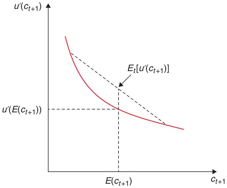
Now assume, in addition to the typical \(u^{\prime}>0\) and \(u^{\prime \prime}<0\), that \(u^{\prime \prime \prime}>0\). This last condition is new and says that marginal utility is convex. This seems to be a very realistic assumption. It means that the marginal utility of consumption grows very fast as consumption approaches very low levels. Roughly speaking, people with convex marginal utility will be very concerned with very low levels of consumption. Figure 12.1 shows how marginal utility behaves if this condition is met.
Notice that for a quadratic utility
\[ E\left[u^{\prime}(c)\right]=u^{\prime}(E[c]) . \tag{12.27}\]
But the graph shows clearly that if marginal utility is convex then
\[ E\left[u^{\prime}(c)\right]>u^{\prime}(E[c]), \tag{12.28}\]
and that the stronger the convexity, the larger the difference. The bigger \(E\left[u^{\prime}(c)\right]\) is, the bigger \(c_{t+1}\) needs to be to keep the expected future utility equal to \(u^{\prime}(c)\), the marginal utility of consumption today. Imagine, for example that you expect one of your consumption possibilities for next period to be zero. If marginal utility at zero is \(\infty\) then \(E\left[u^{\prime}(c)\right]\) will also be \(\infty\), and therefore you want to increase future consumption as much as possible to bring this expected marginal utility down as much as possible. In the extreme you may choose not to consume anything today! This means that you keep some extra assets, a buffer stock, to get you through the possibility of really lean times. This is what is called precautionary savings. Precautionary savings represents a departure from the permanent income hypothesis, in that it will lead individuals to save more than would be predicted by the latter, because of uncertainty.
The Caballero model
Caballero (1990) provides a nice example that allows for a simple solution. Consider the case of a constant absolute risk aversion function.
\[ u\left(c_{t}\right)=-\frac{1}{\theta} e^{-\theta c_{t}} . \tag{12.29}\]
Assuming that the interest rate is equal to the discount rate for simplification, this problem has a traditional Euler equation of the form
\[ e^{-\theta c_{t}}=E_{t}\left[e^{-\theta c_{t+1}}\right] . \tag{12.30}\]
Caballero proposes a solution of the form
\[ c_{t+1}=\Gamma_{t}+c_{t}+v_{t+1}, \tag{12.31}\]
where \(v\) is related to the shock to income, the source of uncertainty in the model. Replacing in the Euler equation gives
\[ e^{-\theta c_{t}}=E_{t}\left[e^{-\theta\left[\Gamma_{t}+c_{t}+v_{t+1}\right]}\right], \tag{12.32}\]
which, taking logs, simplifies to
\[ \theta \Gamma_{t}=\log E_{t}\left[e^{-\theta v_{t+1}}\right] . \tag{12.33}\]
If \(v\) is distributed \(N\left(0, \sigma_{v}^{2}\right)\), then we can use the fact that \(E e^{x}=e^{E x+\frac{\sigma_{x}^{2}}{2}}\) to find the value of \(\Gamma\) (as the value is constant, we can do away with the subscript) in (12.33):
\[ \theta \Gamma=\log \left[e^{\frac{\theta^{2} \sigma_{v}^{2}}{2}}\right], \tag{12.34}\]
or, simply,
\[ \Gamma=\frac{\theta \sigma_{v}^{2}}{2} . \tag{12.35}\]
This is a very simple expression. It says that even when the interest rate equals the discount rate the consumption profile is upward sloping. The higher the variance, the higher the slope.
The precautionary savings hypothesis is also useful to capture other stylised facts: families tend to show an upward-sloping consumption path while the uncertainties of their labour life get sorted out. Eventually, they reach a point were consumption stabilises and they accumulate assets. Gourinchas and Parker (2002) describe these dynamics. Roughly the pattern that emerges is that families have an increasing consumption pattern until sometime in the early 30s, after which consumption starts to flatten.
12.2 New frontiers in consumption theory
Consumption shows significant deviations from the optimal intertemporal framework. One such deviation is explained by early bias, a tendency to give a stronger weight to present consumption. This leads to time inconsistency in consumption plans. Consumption restrictions, such as requesting a stay period before consumption, may solve the problem.
Though our analysis of consumption has taken us quite far, many consumption decisions cannot be suitably explained with the above framework as it has been found that consumers tend to develop biases that move their decisions away from what the model prescribes. For example, if a family receives an extra amount of money, they will probably allocate it to spending on a wide range of goods and maybe save at least some of this extra amount. Yet, if the family receives the same amount of extra money on a discount on food purchases, it is found that they typically increase their food consumption more (we could even say much more) than if they would have received cash. Likewise, many agents run up debts on their credit cards when they could pull money from their retirement accounts at a much lower cost.
One way of understanding this behaviour is through the concept of mental accounting, a term coined by Richard Thaler, who won the Nobel Prize in economics in 2017. In Thaler’s view, consumers mentally construct baskets of goods or categories. They make decisions based on these categories not as if they were connected by a unique budget constraint, but as if they entailed totally independent decisions.
A similar anomaly occurs regarding defaults or reference points which we mentioned at the end of our Social Security chapter. Imagine organising the task of allocating yellow and red mugs to a
group of people. If you ask people what colour they would like their mugs to be, you will probably get a uniform distribution across colours, say 50% choose yellow and 50% choose red. Now allocate the mugs randomly and let people exchange their mugs. When you do this, the number of exchanges is surprisingly low. The received mug has become a reference point which delivers utility per-se. This type of reference point explains why agents tend to stick to their defaults. Brigitte Madrian has shown that when a \(3 \%\) savings contribution was imposed as default (but not compulsory), six months later \(86 \%\) of the workers remained within the plan, relative to 49% if no plan had been included as default, and 65% stuck to the 3% contribution vs only 4% choosing that specific contribution when such percentage was not pre-established. (In fact, Madrian shows that the effect of defaults is much stronger than providing economic incentives for savings, and much cheaper!)
One of the biases that has received significant attention is what is called present bias. Present bias is the tendency to put more weight to present consumption relative to future consumption. Let’s discuss the basics of this idea.
12.2.1 Present bias
We follow (Beshears et al. 2006) in assuming a model with three periods. In period zero the consumer can buy (but not consume) an amount \(c_{0} \geq 0\) of a certain good. In period one, the consumer can buy more of this good \(\left(c_{1} \geq 0\right)\) and now consume it. Total consumption is
\[ c=c_{0}+c_{1} . \tag{12.36}\]
In period 2, the consumer spends whatever was left on other goods \(x\). The budget constraint can be written as
\[ 1+T=c_{0}\left(1+\tau_{0}\right)+c_{1}\left(1+\tau_{1}\right)+x, \tag{12.37}\]
where \(\tau_{0}\) and \(\tau_{1}\) are taxes over \(c_{0}\) and \(c_{1}\) and \(T\) is a lump sum transfer. Income is assumed equal to 1. \(T=\overline{c_{0}} \tau_{0}+\overline{c_{1}} \tau_{1}\), where the bars indicate the average values for each variable. As the economy is large, these variables are unchanged by the individual decision to consume. Introducing taxes and lump sum transfers is not necessary, but will become useful below to discuss policy. Summing up, the structure is:
Period 0: buys \(c_{0}\) at after tax price of \(\left(1+\tau_{0}\right)\)
Period 1: buys an additional amount \(c_{1}\) at an after tax price of \(\left(1+\tau_{1}\right)\). Consumes \(c=c_{0}+c_{1}\)
Period 2: buys and consumes good \(x\) at price 1 with the remaining resources \(1+T-c_{0}\left(1+\tau_{0}\right)-\) \(c_{1}\left(1+\tau_{1}\right)\).
Time inconsistency in consumer’s behaviour
The key assumption is that the consumer has a quasi-hyperbolic intertemporal discount factor with sequence: \(1, \beta \frac{1}{1+\rho}, \beta\left(\frac{1}{1+\rho}\right)^{2}, \beta\left(\frac{1}{1+\rho}\right)^{3}\). We assume \(0 \leq \beta \leq 1\) to capture the fact that the consumer discounts more in the short run than the long run. As we will see, this will produce preferences that are not consistent over time. In addition, we will assume the good provides immediate satisfaction but a delayed cost (a good example would be smoking or gambling).
Let’s assume that the utility of consuming \(c\) is
\[ E u_{0}(c, x)=E\left[\beta \frac{1}{1+\rho}(\alpha+\Delta) \log (c)-\beta\left(\frac{1}{1+\rho}\right)^{2} \alpha \log (c)+\beta\left(\frac{1}{1+\rho}\right)^{2} x\right], \tag{12.38}\]
where \(\Delta\) and \(\alpha\) are fixed taste-shifters. The utility from \(x\) is assumed linear, as it represents all other goods.
For simplicity, we assume \(\frac{1}{1+\rho}=1\). Expected utility as seen in period zero is
\[ E u_{0}(c, x)=E \beta[\Delta \log (c)+x] . \tag{12.39}\]
Notice that the delayed consumption penalty disappears when seen from afar. In period 1, the utility function is
\[ u_{1}(c, x)=(\Delta+\alpha) \log (c)-\beta \alpha \log (c)+\beta x . \tag{12.40}\]
Notice that relative utility between the good \(c\) and \(x\) is not the same when seen at time 0 and when seen at time 1. At period zero, the other goods were not penalised relative to \(c\), but from the perspective of period 1 the benefits of consumption are stronger because satisfaction is immediate relative to the delayed cost and relative to the utility of other goods to which the present bias applies. This will lead to time inconsistency.
Precommitment
Imagine consumption is determined at time zero and for now \(\tau_{0}=\tau_{1}=0\). This would give the optimal consumption ex-ante. Maximising (12.39) subject to (12.37) can easily be shown to give
\[ \frac{\Delta}{c}=1 . \tag{12.41}\]
Notice that this implies \(c=\Delta\) and \(x=1-\Delta\). Thus, expected utility as of period 0 is
\[ E u_{0}(c, x)=E \beta[\Delta \log (\Delta)]+\beta(1-\Delta) . \tag{12.42}\]
This will be our benchmark.
The free equilibrium
Keeping \(\tau_{0}=\tau_{1}=0\), now imagine that consumption is chosen in period 1. This is obtained maximising (12.40) subject to (12.37). This gives
\[ \frac{\alpha(1-\beta)+\Delta}{c}=\beta . \tag{12.43}\]
Notice that now \(c=\frac{\alpha(1-\beta)+\Delta}{\beta}\) which can easily be shown to be higher than the value obtained in the precommitment case. From the perspective of period 0, the marginal utility of \(c\) is now smaller than the utility of consuming \(x\). Thus, this free equilibrium is not first-best optimal at least from the perspective of period zero.
Optimal regulation: Las Vegas or taxation?
Are there policies that may restore the first-best equilibrium from the perspective of period zero utility?
One option is an early decision rule that allows the purchase of \(c\) only during period zero. This is like having an infinite tax in period 1. A well-known application of this policy is, for example, to move gambling activities far away from living areas (e.g. Las Vegas). This way, the consumer decides
on the consumption without the urgency of the instant satisfaction. This case trivially replicates the precommitment case above and need not be repeated here.
This outcome can also be replicated with optimal taxation. To see how, let’s consider a tax policy of the form \(\tau_{0}=\tau_{1}=\tau\). In order to solve this problem, let’s revisit the maximisation of (12.40) subject to (12.37). The solution for \(c\) gives
\[ c=\frac{\alpha(1-\beta)+\Delta}{\beta(1+\tau)} . \tag{12.44}\]
To obtain the optimal \(\tau\), replace (12.44) in (12.39) and maximise with respect to \(\tau\). The first order condition gives :
\[ -\frac{\Delta}{1+\tau}+\frac{\alpha(1-\beta)+\Delta}{\beta(1+\tau)^{2}}=0, \tag{12.45}\]
which gives the optimal tax rate
\[ \tau=\left(\frac{\alpha}{\Delta}+1\right)\left(\frac{1}{\beta}-1\right), \tag{12.46}\]
which delivers \(c=\Delta\), replicating the optimal equilibrium. So a tax policy can do the trick. In fact, with no heterogeneity both policies are equivalent.
Things are different if we allow for heterogeneity. Allow now for individual differences in \(\Delta\). We can repeat the previous steps replacing \(\Delta\) with \(E[\Delta]\), and get the analogous conditions
\[ \beta\left[-\frac{E[\Delta]}{1+\tau}+\frac{\alpha(1-\beta)+E[\Delta]}{\beta(1+\tau)^{2}}\right]=0, \tag{12.47}\]
which gives the same tax rate
\[ \tau=\left(\frac{\alpha}{E(\Delta)}+1\right)\left(\frac{1}{\beta}-1\right) . \tag{12.48}\]
With heterogeneity, consumers will move towards the first best but faced with a unique tax rate will consume different amounts. Notice that \(\beta[\Delta \log (c)+(1-c)]<\beta[\Delta \log (\Delta)+(1-\Delta)]\) for all \(c \neq \Delta\), which happens to the extent that \(E[\Delta] \neq \Delta\). As this happens for a nonzero mass of consumers if heterogeneity is going to be an issue at all:
\[ E u_{0}=E \beta[\Delta \log (c)+1+T-c(1+\tau)]=E \beta[\Delta \log (c)+1-c] \tag{12.49}\]
\[ <E \beta[\Delta \log (\Delta)+1-\Delta] . \tag{12.50}\]
The result is quite intuitive, as each consumer knows its own utility. An early decision mechanism is superior to a tax policy because each individual knows his own utility and attains the first best with the early decision mechanism.
These biases have generated significant attention in recent years, generating important policy recommendations.
12.3 Macroeconomics and finance
While typical corporate finance uses asset prices to explain investment or financing decisions, macrofinance attempts to understand asset prices in a general equilibrium format, i.e. in a way that is consistent with the aggregate outcomes of the economy. The basic pricing equation \(r_{t+1}^{i}-r_{t+1}^{f}=\frac{a \cdot \operatorname{cov}\left(1+r_{t+1}^{i}, c_{t+1}\right)}{E_{t}\left(u^{\prime}\left(c_{t+1}\right)\right)}\) is remarkable; expected returns are not associated with volatility but to the correlation with the stochastic discount factor.
We’ve come a long way in understanding consumption. Now it is time to see if what we have learnt can be used to help us understand what asset prices should be in equilibrium.
To understand this relationship, we can use Lucas’s (1978) metaphor: imagine a tree that provides the economy with a unique exogenous income source. What is this tree worth? Optimal consumption theory can be used to think about this question, except that we turn the analysis upside down. Typically, we would have the price of an asset and have the consumer choose how much to hold of it. But in the economy the amount held and the returns of those assets are given because they are what the economy produces. So here we will use the FOCs to derive what price makes those exogenous holdings optimal. By looking at the FOCs at a given equilibrium point as an asset pricing equation allows us to go from actual consumption levels to asset pricing. Let’s see an example.
Start with the first order condition for an asset that pays a random return \(r_{t+1}^{i}\) :
\[ u^{\prime}\left(c_{t}\right)=\frac{1}{1+\rho} E_{t}\left[\left(1+r_{t+1}^{i}\right) u^{\prime}\left(c_{t+1}\right)\right] \quad \forall i . \tag{12.51}\]
Remember that
\[ \operatorname{cov}(x, y)=E(x y)-E(x) E(y), \tag{12.52}\]
so, applying this equation to (12.51), we have that
\[ u^{\prime}\left(c_{t}\right)=\frac{1}{1+\rho}\left\{E_{t}\left(1+r_{t+1}^{i}\right) E_{t}\left(u^{\prime}\left(c_{t+1}\right)\right)+\operatorname{cov}\left(1+r_{t+1}^{i}, u^{\prime}\left(c_{t+1}\right)\right)\right\} . \tag{12.53}\]
This is a remarkable equation. It says that you really don’t care about the variance of the return of the asset, but about the covariance of this asset with marginal utility. The variance may be very large, but, if it is not correlated with marginal utility, the consumer will only care about expected values. The more positive the correlation between marginal utility and return means a higher right-hand side, and, therefore, a higher value (more utility). Notice that a positive correlation between marginal utility and return means that the return is high when your future consumption is low. Returns, in short, are better if they are negatively correlated with your income; and if they are, volatility is welcomed!
As simple as it is, this equation has a lot to say, for example, as to whether you should own your house, or whether you should own stocks of the company you work for. Take the example of your house. The return on the house are capital gains and the rental value of your house. Imagine the economy booms. Most likely, prices of property and the corresponding rental value goes up. In these cases your marginal utility is going down (since the boom means your income is going up), so the correlation between returns and marginal utility is negative. This means that you should expect housing to deliver a very high return (because its hedging properties are not that good). Well, that’s right on the dot. Remember our mention to Kaplan et al. (2014) in Chapter 8, who show that housing has an amazingly high return. (There may be other things that play a role in the opposite direction, as home ownership provides a unique sense of security and belonging, which our discussion of precautionary
savings indicates can be very valuable.).3 Buying stocks of the firm you work in is a certain no go, so, to rationalise it, you need to appeal to asymmetric information, or to some cognitive bias that makes you think that knowing more about this asset makes you underestimate the risks. In fact, optimal policy would indicate you should buy the stock of your competitor.4
So far, we have been thinking of interest rates as given and consumption as the variable to be determined. However, if all individuals are optimising, equilibrium returns to assets will have to satisfy the same conditions. This means we can think of equation (12.53) as one of equilibrium returns. To make things simple, assume once again that \(u(c)=c-\frac{a c^{2}}{2}\). Then (12.53) becomes:
\[ u^{\prime}\left(c_{t}\right)=\frac{1}{1+\rho}\left\{E_{t}\left(1+r_{t+1}^{i}\right) E_{t}\left(u^{\prime}\left(c_{t+1}\right)\right)-a \cdot \operatorname{cov}\left(1+r_{t+1}^{i}, c_{t+1}\right)\right\}, \tag{12.54}\]
which can also be written as
\[ E_{t}\left(1+r_{t+1}^{i}\right)=\frac{1}{E_{t}\left(u^{\prime}\left(c_{t+1}\right)\right)}\left\{(1+\rho) u^{\prime}\left(c_{t}\right)+a \cdot \operatorname{cov}\left(1+r_{t+1}^{i}, c_{t+1}\right)\right\} . \tag{12.55}\]
Notice that for a risk-free asset, for which \(\operatorname{cov}\left(1+r_{t+1}^{f}, c_{t+1}\right)=0\), we will have
\[ \left(1+r_{t+1}^{f}\right)=\frac{(1+\rho) u^{\prime}\left(c_{t}\right)}{E_{t}\left(u^{\prime}\left(c_{t+1}\right)\right)} . \tag{12.56}\]
Before proceeding, you may want to ponder on an interesting result. Notice that in the denominator you have the expected marginal utility of future consumption. This produces two results. If consumption growth is high, the interest rate is higher (if \(c_{t+1}\) is big, its marginal utility is low). But at the same time, notice that if the volatility of consumption is big, then the denominator is bigger (remember our discussion of precautionary savings). To see this, imagine that under some scenarios \(c_{t+1}\) falls so much that the marginal utility becomes very large. In higher volatility economies, the risk-free rate will be lower!
So, using (12.55) in (12.56) we obtain
\[ E_{t}\left(1+r_{t+1}^{i}\right)-\left(1+r_{t+1}^{f}\right)=\frac{a \cdot \operatorname{cov}\left(1+r_{t+1}^{i}, c_{t+1}\right)}{E_{t}\left(u^{\prime}\left(c_{t+1}\right)\right)}, \tag{12.57}\]
\[ E_{t}\left(r_{t+1}^{i}\right)-r_{t+1}^{f}=\frac{a \cdot \operatorname{cov}\left(1+r_{t+1}^{i}, c_{t+1}\right)}{E_{t}\left(u^{\prime}\left(c_{t+1}\right)\right)} . \tag{12.58}\]
This equation states that the premia of an asset is determined in equilibrium by its covariance with aggregate consumption.
12.3.1 The consumption-CAPM
We show that the basic pricing equation can be written as \(r_{t+1}^{i}-r_{t+1}^{f}=\frac{\operatorname{cov}\left(z_{t+1}^{i}, z_{t+1}^{m}\right)}{\operatorname{var}\left(z_{t+1}^{m}\right)}\left[r_{t+1}^{m}-r_{t+1}^{f}\right]\). Risk premia depend on the asset’s covariance with market returns with a coefficient called \(\beta\) that can be computed by running a regression between individual and market returns. This is the so-called capital asset pricing model (CAPM).
Consider now an asset called “the market” that covaries negatively with marginal utility of consumption (as the market represents the wealth of the economy, consumption moves with it, and therefore in the opposite direction as the marginal utility of consumption). That is,
\[ u^{\prime}\left(c_{t+1}\right)=-\gamma z_{t+1}^{m} . \tag{12.59}\]
Applying (12.58) to this asset, we have
\[ r_{t+1}^{m}-r_{t+1}^{f}=\frac{\gamma \cdot \operatorname{var}\left(z_{t+1}^{m}\right)}{E_{t}\left(u^{\prime}\left(c_{t+1}\right)\right)} . \tag{12.60}\]
Consider now an individual asset with return \(z_{t+1}^{i}\). Applying the same logic we have that
\[ r_{t+1}^{i}-r_{t+1}^{f}=\frac{\gamma \cdot \operatorname{cov}\left(z_{t+1}^{i}, z_{t+1}^{m}\right)}{E_{t}\left(u^{\prime}\left(c_{t+1}\right)\right)} . \tag{12.61}\]
Combining both equations (just replace \(E_{t}\left(u^{\prime}\left(c_{t+1}\right)\right)\) from (12.60) into (12.61), we have that
\[ r_{t+1}^{i}-r_{t+1}^{f}=\frac{\operatorname{cov}\left(z_{t+1}^{i}, z_{t+1}^{m}\right)}{\operatorname{var}\left(z_{t+1}^{m}\right)}\left[r_{t+1}^{m}-r_{t+1}^{f}\right] . \tag{12.62}\]
You may have seen something very similar to this equation: it is the so-called CAPM, used to determine the equilibrium return of an asset. The formula says that the asset will only get a premia for the portion of its variance that is not diversifiable. An asset can have a very large return, but if the correlation of the return with the market is zero, the asset will pay the risk-free rate in spite of all that volatility! Another way of saying this is that all idiosyncratic (i.e. diversifiable by holding a sufficiently large portfolio) risk is not paid for. This is the reason you should typically not want to hold an individual asset: it will carry a lot of volatility you are not remunerated for. The popularity of the CAPM model also hinges on how easy it is to compute the slope of the risk premia: it is just the regression coefficient obtained from running the return of the asset (relative to the risk free) and the market return. The value of that coefficient is called \(\beta\).
This version, derived from the optimal behaviour of a consumer under uncertainty, is often referred to as Consumption-based CAPM (C-CAPM).
12.3.2 Equity premium puzzle
The premia for equities is given by \(E\left(r^{i}\right)-\bar{r}=\theta \operatorname{cov}\left(r^{i}, g^{c}\right)\). But this does not hold in the data unless risk aversion is unreasonably high. This is the so-called equity premium puzzle.
Our asset pricing model can help us think about some asset pricing puzzles that have long left economists and finance practitioners scratching their heads. One such puzzle is the equity premium puzzle.
The puzzle, in the U.S., refers to the fact that equities have exhibited a large premia (around \(6 \%\) on average) relative to bonds, and this premia has remained relatively constant for about 100 years. As equities are riskier than bonds a premia is to be expected. But does 6% make sense? If an asset earns \(6 \%\) more than another, it means that the asset value will be \(80 \%\) higher at the end of 10 years, \(220 \%\) more at the end of 20 years, 1740% higher at the end of 50 years, and 33.800% higher at the end of 100 years! You get the point; there is no possible risk aversion coefficient that can deliver these differences as an equilibrium spread.
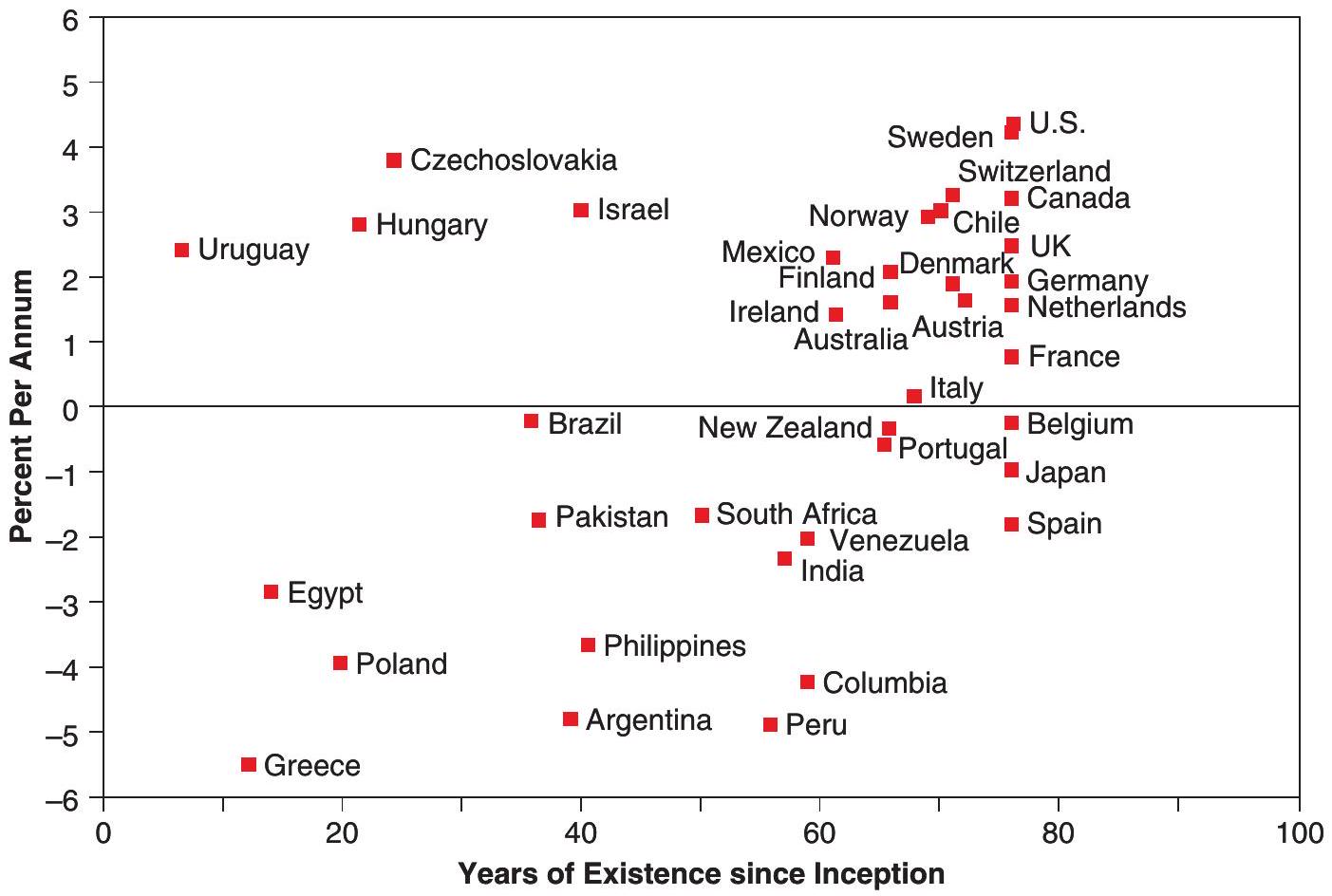
Figure 12.2, taken from Jorion and Goetzmann (1999), shows that the equity premium puzzle is a common occurrence, but does not appear in all countries. In fact the U.S. seems to be the country where its result is most extreme.
To have more flexibility, we need to move away from a quadratic utility function and use a more general CRRA utility function instead. Now our FOC looks like
\[ c_{t}^{-\theta}=\frac{1}{1+\rho} E_{t}\left[\left(1+r_{t+1}^{i}\right) c_{t+1}^{-\theta}\right], \tag{12.63}\]
which can be written as
\[ 1+\rho=E_{t}\left[\left(1+r_{t+1}^{i}\right) \frac{c_{t+1}^{-\theta}}{c_{t}^{-\theta}}\right]=E_{t}\left[\left(1+r_{t+1}^{i}\right)\left(1+g^{c}\right)^{-\theta}\right] . \tag{12.64}\]
Take a second order expansion of the term within the square brackets on the RHS at \(g=r=0\) (notice that in this case the usual \(\Delta r\) becomes \(r\), and \(\Delta g\) becomes \(g\) )
\[ \begin{aligned} 1+\left(1+g^{c}\right)^{-\theta} r+(1+r)(-\theta)\left(1+g^{c}\right)^{-\theta-1} g^{c}+(-\theta)\left(1+g^{c}\right)^{-\theta-1} g^{c} r+ &\\ +\frac{1}{2}(1+r)(-\theta)(-\theta-1)\left(1+g^{c}\right)^{-\theta-2}\left(g^{c}\right)^{2} . & \end{aligned} \tag{12.65}\]
At \(r=g=0\) (but keeping the deviations), this simplifies to
\[ 1+r-\theta g^{c}-\theta g^{c} r+\frac{1}{2} \theta(\theta+1)\left(g^{c}\right)^{2} . \tag{12.66}\]
With this result, and using (12.52), we can approximate (12.64) as
\[ \rho \cong E\left(r^{i}\right)-\theta E\left(g^{c}\right)-\theta\left\{E\left(r^{i}\right) E\left(g^{c}\right)+\operatorname{cov}\left(r^{i}, g^{c}\right)\right\}+\frac{1}{2} \theta(\theta+1)\left\{E\left(g^{c}\right)^{2}+\operatorname{var}\left(g^{c}\right)\right\}, \tag{12.67}\]
where we can drop the quadratic terms \(\left(E\left(r^{i}\right) E\left(g^{c}\right)\right.\) and \(\left.E\left(g^{c}\right)^{2}\right)\) as these may be exceedingly small. This simplifies again to
\[ \rho \cong E\left(r^{i}\right)-\theta E\left(g^{c}\right)-\theta \operatorname{cov}\left(r^{i}, g^{c}\right)+\frac{1}{2} \theta(\theta+1) \operatorname{var}\left(g^{c}\right) . \tag{12.68}\]
For a risk free asset, for which \(\operatorname{cov}\left(r^{i}, g^{c}\right)=0\), the equation becomes
\[ \bar{r}=\rho+\theta E\left(g^{c}\right)-\frac{1}{2} \theta(\theta+1) \operatorname{var}\left(g^{c}\right), \tag{12.69}\]
which again shows the result that the higher the growth rate, the higher the risk free rate, and that the bigger the volatility of consumption the lower the risk free rate! Using (12.69) in (12.68) we obtain
\[ E\left(r^{i}\right)-\bar{r}=\theta \operatorname{cov}\left(r^{i}, g^{c}\right) . \tag{12.70}\]
This is the risk premia for an asset \(i\). We will see that this equation is incompatible with the observed spread on equities (6% per year). To see this, notice that from the data we know that \(\sigma_{g^{c}}=3.6 \%\), \(\sigma_{r^{i}}=16.7 \%\), and \(\operatorname{corr}_{r^{i}, g^{c}}=.40\). This implies that
\[ c o v_{r^{i}, g^{c}}=(.40) \cdot(.036) \cdot(.167)=0.0024 . \tag{12.71}\]
Now we can plug this into (12.70) to get that the following relation has to hold,
\[ 0.06=\theta \cdot 0.0024 \tag{12.72}\]
and this in turn implies \(\theta=25\), which is considered too high and incompatible with standard measures of risk aversion (that are closer to 2). Mehra and Prescott (1985) brought this issue up and kicked off a large influx of literature on potential explanations of the equity premium. In recent years the premium seemed, if anything, to have increased even further. But be careful, the increase in the premia may just reflect the convergence of the prices to their equilibrium without the premia. So we can’t really say how it plays out from here on.
12.4 What next?
Perfect or not, the idea of consumption smoothing has become pervasive in modern macroeconomics. Many of you may have been taught with an undergraduate textbook using a consumption function \(C=a+b Y\), with a so-called marginal propensity to consume from income equal to \(b\). Modern macroeconomics, both in the version with and without uncertainty, basically states that this equation does not make much sense. Consumption is not a function of current income, but of intertemporal wealth. The distinction is important because it affects how we think of the response of consumption to shocks or taxes. A permanent tax increase will imply a one to one reduction in consumption with no effect on aggregate spending, while transitory taxes have a more muted effect on consumption. These
intertemporal differences are indistinguishable in the traditional setup but essential when thinking about policy.
The theory of consumption has a great tradition. The permanent income hypothesis was initially stated by Milton Friedman who thought understanding consumption was essential to modern macroeconomics. Most of his thinking on this issue is summarised in his 1957 book A Theory of the Consumption Function (Friedman (1957), though this text, today, would be only of historical interest. The life cycle hypothesis was presented by Modigliani and Brumberg (1954), again, a historical reference.
Perhaps a better starting point for those interested in consumption and savings is Angus Deaton’s (1992) Understanding Consumption.
For those interested in exploring value function estimations you can start easy be reviewing Chiang’s (1992) Elements of Dynamic Optimization, before diving into Ljungqvist and Sargent (2018) Recursive Macroeconomic Theory. Miranda and Fackler (2004) Applied Computational Economics and Finance is another useful reference. Eventually, you may want to check out Sargent and Stachurski (2014) Quantitative Economics, which is graciously available online at https://quantecon. org/lectures/.
There are also several computer programs available for solving dynamic programming models. The CompEcon toolbox (a MATLAB toolbox accompanying Miranda and Fackler (2004) textbook), and the quant-econ website by Sargent and Stachurski with Python and Julia scripts.
If interested in macrofinance, the obvious reference is Cochrane’s Asset Pricing (2009), of which there have been several editions. Sargent and Ljungqvist provide two nice chapters on asset pricing theory and asset pricing empirics that would be a wonderful next step to the issues discussed in this chapter. If you want a historical reference, the original Mehra and Prescott (1985) article is still worth reading.
References
Beshears, J., Choi, J. J., Laibson, D., & Madrian, B. (2006). Early decisions: A regulatory framework. National Bureau of Economic Research.
Caballero, R. J. (1990). Consumption puzzles and precautionary savings. Journal of Monetary Economics, 25(1), 113-136.
Friedman, M. (1957). A theory of the consumption function. Princeton University Press.
Ganong, P. & Noel, P. (2019). Consumer spending during unemployment: Positive and normative implications. American Economic Review, 109(7), 2383-2424.
Gourinchas, P.-O. & Parker, J. A. (2002). Consumption over the life cycle. Econometrica, 70(1), 47-89.
Hall, R. E. (1978). Stochastic implications of the life cycle-permanent income hypothesis: Theory and evidence. Journal of Political Economy, 86(6), 971-987.
Jorion, P. & Goetzmann, W. N. (1999). Global stock markets in the twentieth century. The Journal of Finance, 54(3), 953-980.
Kaplan, G., Violante, G. L., & Weidner, J. (2014). The wealthy hand-to-mouth. National Bureau of Economic Research. https://www.nber.org/system/files/working_papers/w20073/w20073.pdf.
Ljungqvist, L. & Sargent, T. J. (2018). Recursive macroeconomic theory. MIT Press.
Lucas Jr, R. E. (1978). Asset prices in an exchange economy. Econometrica, 1429-1445.
Mehra, R. & Prescott, E. C. (1985). The equity premium: A puzzle. Journal of Monetary Economics, 15(2), 145-161.
Miranda, M. J. & Fackler, P. L. (2004). Applied computational economics and finance. MIT Press.
Modigliani, F. & Brumberg, R. (1954). Utility analysis and the consumption function: An interpretation of cross-section data. Post Keynesian Economics. Rutgers University Press, 388-436.
Sargent, T. & Stachurski, J. (2014). Quantitative economics. https://quantecon.org/lectures/.
Shea, J. (1995). Myopia, liquidity constraints, and aggregate consumption: A simple test. Journal of Money, Credit and Banking, 27(3), 798-805.
Later on in the chapter we will allow the return \(r\) also to be stochastic. If such is the case it should be inside the square brackets. We will come back to this shortly.↩︎
You can check easily that this specification has positive marginal utility (or can be so), and negative second derivative of utility relative to consumption.↩︎
It might also be because policy, such as federal tax deductibility of mortgage interest (and not of rental payments), encourages excessive home ownership.↩︎
We can also appeal to irrationality: people may convince themselves that the company they work for is a can’t miss investment. And how often have you heard that paying rent is a waste of money?↩︎